Abstract

We study the universality between a discrete spin model with icosahedral symmetry and the $O(3)$ model in two dimensions. For this purpose we study numerically the renormalized two-point functions of the spin field and the four point coupling constant. We find that those quantities seem to have the same continuum limits in the two models. This has far reaching consequences, because the icosahedron model is not asymptotically free in the sense that the coupling constant proposed by Lüscher, Weisz and Wolff [1] does not approach zero in the short distance limit. By universality this then also applies to the $O(3)$ model, contrary to the predictions of perturbation theory.

1 Introduction

The subject of the enhancement of a discrete symmetry to a continuous one at large distances is important both theoretically and phenomenologically. Indeed, even if there are good grounds to expect that a certain material is well described by some model enjoying $O(N)$ symmetry, one may wonder what might be the effect of anisotropies. This question was addressed in 1977 by José et al [2] for the $O(2)$ nonlinear $\sigma$ model. Nonrigorous renormalization group arguments led them to the conclusion that in two dimensions ($2D$) the discrete symmetry $Z_{N}$ should be enhanced to full $O(2)$ invariance if $N\geq 5$ for $\beta$ (inverse temperature) not too large. For $N$ sufficiently large, the occurrence of this phenomenon was proven rigorously by Fröhlich and Spencer in 1981 [3], who showed that there exists a range of temperatures in which spin correlation functions decay algebraically and are $O(2)$ invariant. Fröhlich and Spencer proved also that a similar phenomenon of discrete abelian symetry enhancement occurs in $4D$ gauge theories.

For a long time, the consensus was that no symmetry enhancement should occur in nonabelian models. The main reason appears to have been the belief that for continous symmetries, these models exhibit asymptotic freedom (AF). The discrete models, known rigorously to undergo phase transitions at nonzero temperature, did not seem likely to be AF, hence had to be different. A proposal for nonabelian symmetry enhancement came however from Newman and Schulman [4]. Their argument was based on the fact that if the discrete symmetry group is sufficiently large, any 4-th order polynomial invariant under the discrete group is also invariant under the continuous group in which it is contained. While this is an undisputable mathematical fact, the question was why 4-th order? Their heuristic answer was that the renormalization group flow was expected to be free of bifurcations as the dimension $D$ was varied between 2 and 4. So if one started just below $D=4$, where the most one could have is a $\phi^{4}$ interaction (higher powers being irrelevant), this symmetry enhancement should persist down to $D=2$. Since however in $D=2$ all polynomials in $\phi$ are relevant and it is easy to write down such polynomials possessing only a discrete symmetry, and to construct the corresponding $P(\phi)_{2}$ models, the validity of the argument of Newman and Schulman remains unclear.

A different heuristic argument in favor of symmetry enhancement for abelian as well as nonabelian groups was put forward by Patrascioiu in 1985 [5]. For spin models, his argument went as follows: at sufficiently low temperatures, there exists a phase with long range order (l.r.o.) because, as Peierls showed long ago, given an ordered state, there is not enough free energy to create a domain in which the spin points elsewhere. Now consider a model like $Z_{5}$. As one increases the temperature, clearly the first abundant domains to form would be those in which the spin pointed in a direction immediately neighboring the one chosen by the boundary conditions (b.c.) for the ordered state. For temperatures not too high, the system could form domains inside domains of neighboring spin values. This would be different from the phase at high temperature, where no such restriction between adjacent domains would be required. This scenario does not seem to have anything it do with the model being abelian or not and Patrascioiu suggested that, since it was known to happen in abelian models, it must happen also in nonabelian cases.

Except for the papers quoted above, in the 80s, while it was quite fashionable to replace continous groups with discrete ones in Monte Carlo simulations, everybody seemed to be convinced that the discrete and continuous models belonged to different universality classes. Our interest in the subject was rekindled in 1990 when, together with Richard, we derived a rigorous inequality relating correlation functions in the dodecahedron model to those of $Z_{10}$ [6]. Our result was that for any $\beta$ the dodecahedron model is more ordered than $Z_{10}$ at $0.607^{2}\beta$. Since it is was pretty well established that $Z_{10}$ possess an extended intermediate phase which is $O(2)$ invariant, our inequality implied that provided $\beta_{m}({\it D})>\beta_{c}(Z_{10})$ the dodecahedron must also possess an intermediate massless phase. Here $\beta_{m}({\it D})$ denotes the onset of the l.r.o. phase in the dodecahedron and $\beta_{c}(Z_{10})$ the onset of algebraic decay in $Z_{10}$. We determined numerically these values [7] and concluded that the dodecahedron seemed to possess an intermediate massless phase for $2.15<\beta<2.8$. We conjectured that this phase must enjoy full $O(3)$ invariance.

Intrigued by our findings for the dodecahedron, in the early 90s we looked numerically at the other regular polyhedra. While the cube is obviously equivalent to 3 uncoupled Ising models, hence not a good candidate for exhibiting $O(3)$ invariance, the other 3 regular polyhedra (platonic solids) a priori are. Actually in the scenario advocated by Patrascioiu in 1985 [5], the tetrahedron should not be able to simulate spin waves since its spin gradient can take only one nontrivial value (in fact it is nothing but the 4 state Potts model). The octahedron and the icosahedron could. Our numerics suggested that the octahedron had a first order transition. For the icosahedron the MC data suggested a second order transition from the high temperature phase to the low temperature phase exihibiting l.r.o.; in particular there did not seem to be an extended massless phase, as for the dodecahedron.

That the discrete icosahedral symmetry may be enhanced to $O(3)$ began to become manifest in 1998 when we began extensive numerical investigations of the contiuum limit of the spin 2-point function versus $p/m$ [8] in the dodecahedron model. The original motivation of that study was to compare the lattice continuum limit with the form factor (FF) prediction of Balog and Niedermaier [9]. Since it was not to be expected that the latter could possibly describe the continuum limit of the dodecahedron model, we decided to take data on this model too. To our surprise, the $O(3)$ data seemed to agree with both the FF prediction and with the dodecahedron. Since Balog and Niedermaier had produced a convincing argument [10] that the FF approach incorporates AF and we could not see how a discrete model, freezing at nonzero temperature, could possibly be AF, we decided to refine our data by concentrating on the region $p/m<13$. Our results [11] showed small but statistically significant deviations between $O(3)$ and FF, but excellent agreement between $O(3)$ and the dodecahedron.

The comparison of the FF and $O(3)$ could have been marred by lattice artefacts, a problem to which we will return below. This is why a different comparison was performed by Patrascioiu [12], who computed the renormalized spin 2-point function versus the physical distance $x/\xi$. The results were very similar with the ones we will report here about the icosahedron. They suggested that the dodecahedron and $O(3)$ models share the same continuum limit.

Another reason to investigate the discrete spin models arose in 1999, while in collaboration with Balog, Niedermaier, Niedermayer and Weisz we decided to compare the FF prediction for the renormalized coupling $g_{R}$ (to be defined below) with its lattice continuum limit value. Although our first results [13] suggested excellent agreement, as we continued to reduce the error bars and especially to take data at larger correlation length $\xi\approx 167$, our original extrapolation to the continuum limit became dubious and in our second paper [14] we stated that we could no longer give a reliable number for the lattice continuum limit value of $g_{R}$. In the hope of gaining insight into this issue, we turned again to the discrete models. Corroborating our previous findings regarding $G_{r}(p/m)$ and $G_{r}(x/\xi)$, the data, to be shown later, suggested that $g_{R}$ also agreed in the dodecahedron, icosahedron and $O(3)$ models.

In the course of the debates of our collaboration F. Niedermayer raised the intriguing possibility that maybe indeed all these models do have the same continuum limit, which however is AF. The present paper is our reply to his suggestion. The results were communicated to him already in 1999, hence we were surprised by his recent paper with P. Hasenfratz [15]. In their paper, Hasenfratz and Niedermayer claim that indeed they find strong numerical evidence that the dodecahedron and icosahedron models have the same continuum limit as $O(3)$, but state that, since “overwhelming evidence exists that the $O(3)$ model is AF”, the dodecahedron and icosahedron models must be AF too. The authors do not mention which ‘overwhelming evidence’ they have in mind, but omit the following facts, which in our opinion are relevant to this issue:

• The data for $g_{R}$ in $O(3)$ produced by Balog et al [14] at larger $\xi$ values do not support the $1/\xi$ fit for the lattice artefacts.

• The last report of Balog et al [14] retracted the original prediction $g_{R}=6.77(2)$ and stated that due to uncontrollable lattice artefacts, no continuum value could be given.

• In our recent paper [16], we combined mathematically rigorous arguments with some numerics to conclude that the $O(3)$ model must undergo a transition to a massless phase at finite $\beta$. We then proved rigorously that such a phase transition rules out the existence of AF in the massive continuum limit.

Being based on numerics, any of the above stated facts could be false, but if Hasenfratz and Niedermayer have evidence to that effect, they should put it forth so that it can be scrutinized.

In this paper we will compare the continuum limit of the $O(3)$ model to that of the icosahedron model by comparing the values of $g_{R}$ and of the renormalized spin 2-point function $G_{r}(x/\xi)$. The advantage of the icosahedron model is the existence of a rather well localisable critical point, whereas, as stated above, the dodecahedral model appears to have a soft intermediate phase. To address the issue of AF, we study the value of the Lüscher-Weisz-Wolff (LWW) coupling constant at the critical point. According to LWW, AF requires that the continuum limit of this observable vanishes at short distances. If in fact the icosahedron model has the same continuum limit as $O(3)$, then the LWW coupling constant should vanish at the critical point of the former model. We find excellent evidence that it does not. Thus our conclusion is that either, in spite of the excellent agreement observed for $\xi\approx 121$, $O(3)$ and the icosahedron model have different continuum limits, or neither is AF.

The paper is organized as follows: we first describe the critical properties of the icosahedon model and in particular locate its critical point. This allows us to determine the value of the LWW running coupling at the critical point. Then we move on to the comparison of the icosahedron and the $O(3)$ models. We compare the renormalized coupling constant and the renormalized spin-spin correlation function of the two models and present convincing evidence that they converge to the same continuum limit.

2 Critical Behavior of Icosahedron Model

We first describe the critical properties of the icosahedron model: we locate the critical point and give some estimates of critical exponents. This allows us to determine the value of the Lüscher-Weisz-Wolff (LWW) coupling constant at the critical point, which is independent ot the size $L$ of the lattice, as required by scaling. This (nonzero) value is also the short distance limit of the continuum value of the LWW coupling constant.

The icosahedron model is defined by the standard nearest neighbor coupling between the spins

$$H=-\sum_{\langle ij\rangle}s_{i}\cdot s_{j}$$ (1)

where the spins $s_{i}$ are unit vectors forming the vertices of a regular icosahedron. In suitable coordinates, those 12 vertices are given by

$$e_{k}=(s\cos{2\pi k\over 10},s\sin{2\pi k\over 10},c\cos(\pi k))\ \ (k=1,2,...10);$$ (2)

where

$$s={2\over\sqrt{5}},\ c={1\over\sqrt{5}}$$ (3)

and

$$e_{11}=(0,0,1)\ \ {\rm and}\ \ e_{12}=(0,0,-1)$$ (4)

The model has at least two phases, a high temperature phase with exponential clustering and full symmetry under the icosahedral group $Y$, and a low temperature phase with spontaneous magnetization and 12 coexisting phases, with the magnetization pointing into one of the 12 directions of the icosahedron. At intermediate temperatures there could be in principle a phase with partial breaking of $Y$, but there is no reasonable candidate for a possible unbroken subgroup. There is also the possibility of an extended intermediate phase with no symmetry breaking, but actual enhancement of the symmetry from $Y$ to $O(3)$ as well as only algebraic decay of correlations analogous to the $Z_{N}$ models and the dodecahedron model (see above).

In the icosahedron model the situation seems to be simpler, however: it seems to have a single critical point separating the high and low temperature phases, as we will demonstrate.

To determine the critical point we proceed as follows: we determine the mass gap $m(L)=1/\xi(L)$ in an (ideally infinite) strip of width $L$; in practice we use a finite strip of size $L\times L_{t}$ with $L_{t}>>L$ and measure the effective correlation length defined by

$$\xi(L)={1\over 2\sin(\pi/L_{t})}\sqrt{\chi/G_{1}-1}$$ (5)

where

$$\chi={1\over LL_{t}}\sum_{i,j}\langle s_{i}\cdot s_{j}\rangle,$$ (6)

$$G_{1}={1\over LL_{t}}\sum_{i,j}\langle s_{i}\cdot s_{j}\rangle\exp[{2\pi(i_{1}-j_{1})/L_{t}}].$$ (7)

We then study the behavior of the quantity

$$\bar{g}\equiv{2L\over(N-1)\xi(L)},$$ (8)

which we consider as a function $\bar{g}(z,\xi)$ of $z=L/\xi(\infty)$ and the infinite volume correlation length $\xi(\infty)$. The continuum limit of this quantity for fixed $z$ is the ‘running coupling constant’ introduced by Lüscher, Weisz and Wolff [1] for the $O(N)$ models. In the high temperature phase, where the model has a mass gap $m(\infty)=1/\xi(\infty)$ in the infinite volume limit, $\bar{g}$ will grow linearly with $L$. On the other hand in the low temperature magnetized phase, the mass gap in a finite volume goes to 0 faster than $1/L$, so $\bar{g}$ will decrease to $0$ as $L\to\infty$. At a critical point the model will be scale invariant for large distances and $\bar{g}$ should converge to a finite nonzero limit.

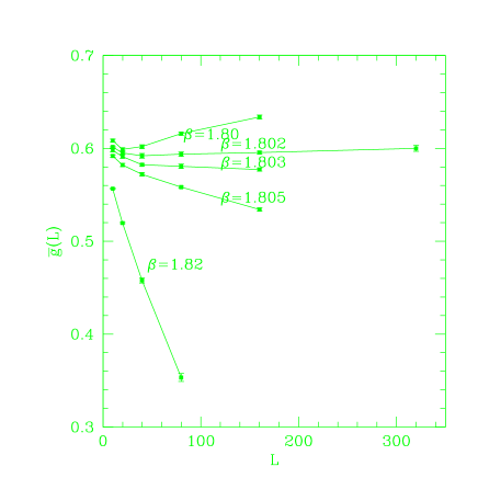
Figure 1: The LWW coupling constant $\bar{g}$ as a function of $L$ for various values of $\beta$

To determine $\bar{g}$ we took data on lattices of size $L\times L_{t}$ with $L_{t}=10L$; $L$ was varied from 10 to 320. Fig.1 (Table 1) shows clearly the dramatic change in behavior between $\beta=1.800$ and $\beta=1.805$. For $\beta=1.802$ $\bar{g}$ shows only some small variation for small $L$ ($L<40$) and stabilizes for larger $L$. So we estimate

$$\beta_{crt}=1.802(1)$$ (9)

where the error is of course somewhat subjective.

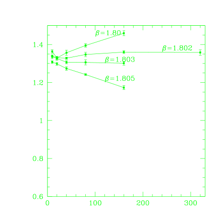
Figure 2: The renormalized coupling for asymmetric $L\times L_{t}$ lattices as a function of $L$ for various values of $\beta$

To corroborate this determination of the critical point, we also measured on the same lattices the renormalized coupling defined as

$$g_{R}=\left({5\over 3}-{g_{4}\over g_{2}^{2}}\right){LL_{t}\over\xi^{2}}.$$ (10)

Here $g_{2}$ is the magnetic susceptibility multiplied by the volume of the lattice $L\times L_{t}$, i.e.

$$g_{2}=\sum_{i,j}\langle s_{i}\cdot s_{j}\rangle$$ (11)

and

$$g_{4}=\sum_{i_{1},i_{2},i_{3},i_{4}}\langle(s_{i_{1}}\cdot s_{i_{2}})(s_{i_{3}}\cdot s_{i_{4}})\rangle$$ (12)

This quantity is also a Renormalization Group (RG) invariant and therefore should also go to a constant for $\beta=\beta_{crt}$. It is well known that in the high temperature phase $g_{R}(L)$ goes to a nontrivial constant for $L\to\infty$, (which as about 6.7, see below) whereas in the magnetized phase it goes to $0$, so one expects a qualitatively similar picture as for $\bar{g}$. The data presented in Table 1 and displayed in Fig.2 confirm this nicely and are consistent with the estimate of $\beta_{crt}$ given above.

Finally we want to see if our determination of $\beta_{crt}$ is consistent with a singularity in the thermodynamic values of the correlation length $\xi$ and the susceptibility $\chi$. We therefore measured $\xi$ and $\chi$ on lattices with $L/\xi\approx 7$ for various values of $\beta<1.802$; our data are given in Tab.2 . There is a row listing the number of runs; a run consists of 100,000 cluster updates for thermalization followed by 20,000 sweeps of the lattice for measurements. Each run is started independently with a randomly chosen new configuration.

To describe the critical behavior of the data for $\xi$ and $\chi$ two types of fits were tried: firstly a Kosterlitz type fit with an exponential singularity

$$\xi=C_{\xi}\exp\left(-a_{\xi}\over\sqrt{\beta_{crt}-\beta}\right),\ \ \chi=C_{\chi}\exp\left(-a_{\chi}\over\sqrt{\beta_{crt}-\beta}\right),$$ (13)

and secondly a power law fit of the type

$$\xi=C_{\xi}(\beta_{crt}-\beta)^{-\nu},\ \ \chi=C_{\chi}(\beta_{crt}-\beta)^{-\gamma}$$ (14)

or similar ones in $1/\beta$. Both types of fit are not very good, with similar quite large values of $\chi^{2}$ and they do not allow a very precise determination of the fit parameters. The reason seems to be the following: the asymptotic singular behavior seems to have significant subleading contributions, which however cannot be well determined with only 5 values of $\beta$. Trying to fit our very precise data with functions that do not describe the behavior with similar accuracy necessarily leads to a poor fit quality, even though visually the data may be very well described (see Fig.3).

The Kosterlitz type fit leads to predictions of $\beta_{crt}\approx 1.93$, which is unacceptably large – this value is deeply in the magnetized phase. The power law fits, on the other hand, give values of $\beta_{crt}$ quite close to our preferred value 1.802 . By playing with the number of parameters and fitting in $1/\beta$ as well as $\beta$ we obtain quite spread in the values of the exponents; they fall into the intervals

$$\nu=1.6-2.0\ \ {\rm and}\ \ \gamma=2.9-3.5$$ (15)

This is consistent with a value of

$$\eta=2-{\gamma\over\nu}\approx.25$$ (16)

which is also favored by the data for spin-spin correlation function (see below).

In Fig.3 we use the best values produced by the power law fit in $1/\beta$ with no subleading corrections, namely

$$\nu=1.717,\ \ \gamma=3.002.$$ (17)

We plot $\xi^{-1/\nu}$ and $\chi^{-1/\gamma}$ vs $\beta$ together with the fits, which are straight lines intersecting the abscissa at $\beta=1.802$. So even though the thermodynamic data for $\xi$ and $\chi$ do not lead to a precise prediction of the critical point and the critical exponents, they are certainly consistent with our determination based on the LWW coupling constant.

We also investigated the possibility that the transition from the high temperature phase to the one with long range order is first order, but we did not find any signal for phase coexistence.

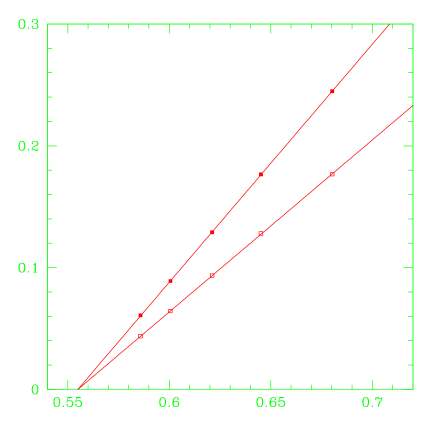
Figure 3: Thermodynamic values of $\xi^{-1/\nu}$ and $\chi^{-1/\gamma}$ with $\nu=1.717$ and $\gamma=3.002$ as functions of $\beta$; the lines are fits.

3 The renormalized coupling in the icosahedron and $O(3)$ models

To check whether the icosahedron and the $O(3)$ model define the same continuum limit, we also determined the renormalized coupling constant $g_{R}$ on thermodynamic lattices. For this purpose we took data on square lattices with $z=L/\xi\approx 7$. To correct for the small finite size effects still present, we determined a finite size scaling curve by taking data at various values of $z=L/\xi$ at $\beta=1.550$ corresponding to $\xi\approx 19.7$. The finite size effects are fitted with the function

$$g_{R}(z)=g_{R}(\infty)(1-d\sqrt{z}\exp(-z).$$ (18)

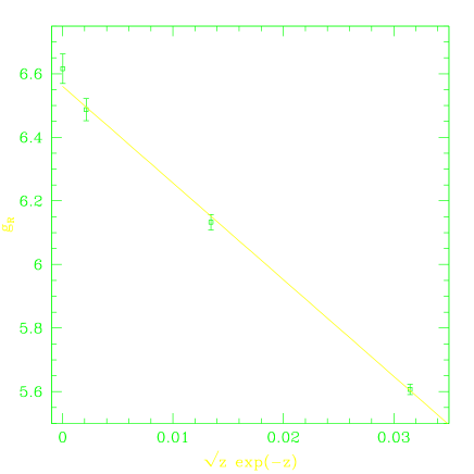
Figure 4: Finite size scaling of $g_{R}$

This behavior is inspired by the spherical model and was successfully used already in [13, 14]. In Fig.4 we show the data at $\beta=1.55$ together with the fit, which has a $\chi^{2}$ per d.o.f. of 1.1 ; the constant $d$ is determined to be

$$d=4.63\pm.15$$ (19)

The results of this fit are then used to extrapolate our data taken with $z\approx 7$ to the thermodynamic values. In Tab.2 we present our data together with the extrapolation.

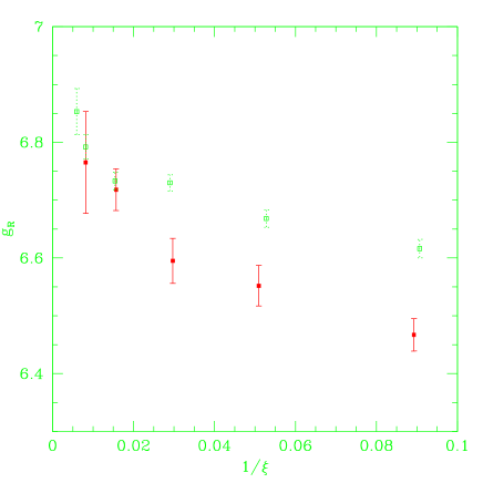
Figure 5: Comparison of $g_{R}$ in the icosahedron and $O(3)$ models Full symbols:icosahedron; open symbols: $O(3)$

Finally we compare our data for $g_{R}$ in the icosahedron model with those we had obtained earlier for the $O(3)$ model [14] and again presented in Tab.2. Fig. 5 shows the thermodynamically extrapolated data for the two models for various values of $\xi$. Even though the lattice artefacts are quite different for the two models, and in spite of the fact that we are not quite sure how one should extrapolate to the continuum limit, the data show that the two models approach each other with increasing $\xi$ (decreasing lattice spacing) and suggest that they will have the same continuum limit.

4 Spin correlation function in the icosahedron and $O(3)$ models

In this section we compare the renormalized spin-spin correlation functions of the icosahedron and the $O(3)$ models. They are defined as

$$G(i/\xi)\equiv{\xi^{2}\over\chi}\langle s(0)\cdot s(i)\rangle$$ (20)

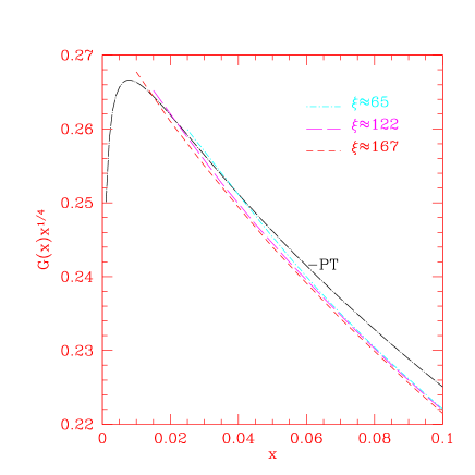
Figure 6: The renormalized spin-spin correlation for the $O(3)$ model for various lattice spacings

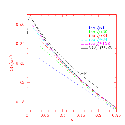
Figure 7: The renormalized spin-spin correlation for the icosahedron model for various lattice spacings: solid line $O(3)$ model for $\xi\approx 122$

The physical distance is

$$x={i\over\xi}$$ (21)

We measured the two-point functions in the icosoahedron model at $\beta=1.47$, 1.55, 1.61, 1.665 and 1.707 corresponding to $\xi\approx$ 11, 20, 34, 64, 122 (see Tab.2). For the $O(3)$ model we used the data from ref.[12] at $\beta=1.8$, 1.9, 1.95 corresponding to $\xi\approx 65$, 122 and 168. In Fig.6 we show $G(x)x^{1/4}$ for the $O(3)$ model together with the 2-loop PT prediction [9]

$$G(x)={1.000034657\over 3\pi^{3}1.001687^{2}}\left[t+\ln t+1.1159+{1\over t}\ln t+{.1159\over t}\right]$$ (22)

where $t=-\ln(x/8)-1$. It can be seen that the data approach their continuum limit from above and deviate considerably from the PT prediction. For $x>0.4$, barring some very slow convergence to the continuum limit, our data suggest that the lattice artefacts are quite small for the large correlation lengths we are using.

In Fig.7 we present $G(x)x^{1/4}$ for the icosahedron model together with the same expression for $O(3)$ at approximately the largest value of $\xi\approx 122$. The lattice artefacts have the opposite sign at least for the lattices with $\xi<122$, i.e. the data are increasing with decreasing lattice spacing. At $\xi\approx 122$ they are already quite close to the corresponding correlation function in the $O(3)$ model. It is therefore reasonable to expect that if we could further refine the lattice we would see that the data follow the behavior of the $O(3)$ model, i.e. the lattice artefacts would change sign and the final approach to the continuum limit would be from above.

It should be stressed that already at $\xi\approx 122$ the icosahedron and $O(3)$ data are much closer to each other than the $O(3)$ data are to the PT prediction.

5 Conclusion: Universality between the icosahedron and $O(3)$ models and asymptotic freedom

We have accumulated strong evidence that the continuum limits of the discrete icosahedron model and the continuous classical Heisenberg ($O(3)$) model describe the same quantum field theory.

As discussed in the introduction, this is one more fact which puts the asymptotic freedom of the $O(3)$ model severely into doubt. The point of view advocated by Hasenfratz and Niedermayer [15], namely that the continuum limit of the discrete icosahedron model should be asymptotically free is untenable in view of our results about the LWW running coupling $\bar{g}$: our data (see Fig.1) indicate that $\bar{g}(L)$ runs to a fixed point value $g^{\ast}\approx.59$ at small distances. Actually to determine the true running coupling, one should take first the continuum limit at fixed $z=L/\xi$ and then the limit $z\to 0$. Since this is not feasible, we instead studied the finite size scaling at and around the critical point and took as our estimate of $g^{\ast}$ the apparent limit

$$\lim_{L\to\infty}m(L)L$$ (23)

at the critical point. Somebody might wonder if it is not possible that the continuum limit shows asymptotic freedom after all; in other words, if it is possible that

$$\lim_{z\to 0}\lim_{\xi\to\infty}\bar{g}(z,\xi)=0\ \ ?$$ (24)

Our data make this extremely unlikely: for fixed $\beta<\beta_{crt}\approx 1.802$ $\bar{g}$ is increasing with $L$ (except for very small lattices) and it is always larger than .59, even at $\beta=1.802$, our estimated critical point. To claim that in the continuum limit $\bar{g}(z,\infty)$ would go to 0 one would have to assume some truly bizarre $L$ dependence at fixed $\beta$. This is illustrated in our Fig.8 which shows some of our data for $\bar{g}$ as a function of $z=L/\xi(\infty)$. We used data at $\beta=1.665$ and 1.707, where we know the correlation length $\xi(\infty)$ quite well, together with the data taken slightly below the estimated critical point, wehre we used the fit appearing in Fig.3 to estimate $\xi(\infty)$. The solid curve is a fit of the form

$$\bar{g}(z)=g^{\ast}+az^{1/2}+bz$$ (25)

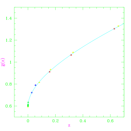
Figure 8: The LWW running coupling for the iscosahedron model as a function of $L/\xi(\infty)$

Since we did not make any effort to control the lattice artefacts and estimate the precise continuum values, this figure should be taken with some caution. It does, however, illustrate nicely the qualitative behavior of the LWW running coupling near the critical point.

To sum up: the universality observed between the icosahedron and the $O(3)$ model gives strong evidence against asymptotic freedom of the latter.

Tab.1:
The LWW running coupling $\bar{g}$ and the renormalized coupling $g_{R}$ as a function of $L$ for various values of $\beta$

$\beta=1.665$:
$L$ 10 20 40 $\bar{g}$ .9121(14) 1.0651(11) 1.3033(21) $g_{R}$ 2.216(13) 2.501(12) 3.080(29)

$\beta=1.707$:
$L$ 10 20 40 80 $\bar{g}$ .8156(9) .9312(12) 1.0882(23) 1.3276(35) $g_{R}$ 1.898(6) 2.213(11) 2.593(23) 3.171(36)

$\beta=1.75$:
$L$ 10 20 $\bar{g}$ .7221(24) .7902(21) $g_{R}$ 1.695(14) 1.841(24)

$\beta=1.80$:
$L$ 10 20 40 80 160 $\bar{g}$ .6083(16) .5989(17) .6018(21) .6158(17) .6337(22) $g_{R}$ 1.363(9) 1.329(9) 1.357(14) 1.395(9) 1.459(13)

$\beta=1.802$:
$L$ 10 20 40 80 160 320 $\bar{g}$ .6015(10) .5951(14) .5919(26) .5938(24) .5955(14) .6000(32) $g_{R}$ 1.340(4) 1.3330(6) 1.328(5) 1.348(11) 1.360(7) 1.358(14)

$\beta=1.803$:
$L$ 10 20 40 80 160 $\bar{g}$ .5979(16) .5912(18) .5823(14) .5807(25) .5772(17) $g_{R}$ 1.335(10) 1.327(10) 1.307(9) 1.306(14) 1.302(10)

$\beta=1.805$:
$L$ 10 20 40 80 160 $\bar{g}$ .5918(13) .5821(17) .5721(19) .5583(8) .5341(19) $g_{R}$ 1.308(7) 1.298(8) 1.274(10) 1.242(4) 1.173(11)

$\beta=1.82$:
$L$ 10 20 40 80 $\bar{g}$ .5566(8) .5196(8) .4578(28) .3533(42) $g_{R}$ 1.213(4) 1.119(4) .964(10) .652(8)

Tab.2:
Correlation length $\xi$, susceptibility $\chi$ and renormalized coupling $g_{R}$ in the high temperature phase of the icosahedron model
$\beta$ 1.470 1.550 1.610 1.665 1.707 $\L$ 80 140 250 500 910 $\xi$ 11.203(5) 19.627(12) 33.655(21) 63.628(33) 122.09(16) $\chi$ 181.88(10) 479.43(36) 1228.04(91) 3774.5(2.1) 12009(17) $g_{R}(L)$ 6.404(28) 6.487(35) 6.546(39) 6.684(36) 6.715(88) $g_{R}(\infty)$ 6.467(28) 6.552(35) 6.595(39) 6.718(36) 6.765(88) # runs 200 100 100 149 28

Tab.3:
Correlation length $\xi$ and renormalized coupling $g_{R}$ in the high temperature phase of the $(O3)$ model (from [14]
$\beta$ 1.5 1.6 1.7 1.8 1.9 1.95 $L$ 80 140 250 500 910 1230 $\xi$ 11.030(7) 18.950(14) 34.500(15) 64.790(26) 122.330(74) 167.71(17) $g_{R}(L)$ 6.553(16) 6.612(15) 6.665(14) 6.691(15) 6.737(21) 6.792(40) $g_{R}(\infty)$ 6.616(16) 6.668(15) 6.730(14) 6.733(15) 6.792(21) 6.853(40) # runs 344 370 367 382 127 68

References

- [1] M. Lüscher, P. Weisz and U. Wolff, Nucl. Phys. B 359 (1991) 221.
- [2] V. José, L. Kadanoff, S. Kirkpatrick and D. Nelson, Phys. Rev. B 16 (1977) 1217.
- [3] J. Fröhlich and T. Spencer, Commun. Math. Phys. 83 (1982) 411.
- [4] C. Newman and L. Schulman, Phys. Rev. B 26 (1982) 3910.
- [5] A. Patrascioiu, Phys. Rev. Lett. 54 (1985) 2292.
- [6] A.Patrascioiu, J. Richard and E.Seiler, Phys. Lett. B241 (1990) 229.
- [7] A.Patrascioiu, J. Richard and E.Seiler, Phys. Lett. B254 (1991) 173.
- [8] A. Patrascioiu and E. Seiler, Phys. Lett. B445 (1998) 160.
- [9] J.Balog and M.Niedermaier, Nucl. Phys. B500 (1997)421.
- [10] J.Balog and M.Niedermaier, Phys.Rev.Lett. 78 (1997) 4151.
- [11] A.Patrascioiu and E.Seiler, Phys. Lett. B430 (1998) 314.
- [12] A.Patrascioiu, Quasi-asymptotic freedom in the teo dimensional model, AZPH-TH-99-01, hep-lat/0002012
- [13] J. Balog, M. Niedermaier, F. Niedermayer, A.Patrascioiu, E. Seiler and P. Weisz, Phys. Rev. D60 (1999) 094508. A.Patrascioiu,
- [14] J. Balog, M. Niedermaier, F. Niedermayer, A.Patrascioiu, E. Seiler and P. Weisz, Nucl.Phys. B583 (2000) 614.
- [15] P. Hasenfratz and F. Niedermayer, Unexpected results in asymptotically free quantum field theories, BUTP-2000-15, hep-lat/0006021.
- [16] A.Patrascioiu and E.Seiler, Absence of asymptotic freedom in nonabelian models, MPI-PHT-2000-07, hep-th/0002153.