Cost of the
Generalised Hybrid Monte Carlo Algorithm
for Free Field Theory

Abstract

We study analytically the computational cost of the Generalised Hybrid Monte Carlo (GHMC) algorithm for free field theory. We calculate the Metropolis acceptance probability for leapfrog and higher-order discretisations of the Molecular Dynamics (MD) equations of motion. We show how to calculate autocorrelation functions of arbitrary polynomial operators, and use these to optimise the GHMC momentum mixing angle, the trajectory length, and the integration stepsize for the special cases of linear and quadratic operators. We show that long trajectories are optimal for GHMC, and that standard HMC is more efficient than algorithms based on Second Order Langevin Monte Carlo (L2MC), sometimes known as Kramers Equation. We show that contrary to naive expectations HMC and L2MC have the same volume dependence, but their dynamical critical exponents are $z=1$ and $z=3/2$ respectively.

Keywords: Hybrid Monte Carlo, HMC, GHMC, Molecular Dynamics, Field Theory, Lattice Field Theory.

PACS numbers: 12.38.Gc, 11.15.Ha, 02.70.Lq

1 Introduction

Hybrid Monte Carlo (HMC) [1] remains the most popular algorithm for simulation of Quantum Chromodynamics (QCD) including the dynamical effects of fermions. It is therefore imperative that we have a detailed understanding of how the computational cost of HMC varies as we change simulation parameters such as the lattice volume and the fermion mass. In this paper we present detailed analytical results for the computational cost of the generalised HMC algorithm for free field theory. We expect many of the results obtained to also be applicable to more general field theories where most of the “modes” are weakly interacting, for example the high momentum modes of asymptotically free theories such as QCD.

In this paper we give detailed descriptions of the techniques we have developed to enable us to calculate fictitious-time evolution operators, Metropolis acceptance probabilities, and autocorrelation functions for arbitrary polynomial operators in GHMC simulations of free field theory. This allows us to minimise the computational cost of such simulations, and to compare the efficiency of various popular limits of GHMC. This paper brings together and extends many results that have been presented previously [2, 3, 4, 5, 6, 7, 8]. The techniques developed for this paper have also been used in several other papers [9, 10, 11, 12].

The structure of this paper is as follows: in Section 2 we describe the Generalised Hybrid Monte Carlo (GHMC) Algorithm and discuss various limiting cases. Section 3 demonstrates that GHMC computations for free field theory are equivalent to GHMC computations for a set of uncoupled harmonic operators with judiciously chosen frequencies. In Section 4 we describe the generalised leapfrog discretisation schemes for the classical equations of motion in fictitious time, and introduce specific parameterisations of the evolution operators in order to facilitate the calculation of the Metropolis acceptance probability in Section 5. In Section 6 we introduce general techniques for calculating Laplace transforms of autocorrelation functions of polynomial operators in free field theory, and present explicit results for arbitrary linear and quadratic operators for several of the limiting cases of GHMC, both for fixed- and exponentially-distributed GHMC trajectory lengths. Section 7 presents a detailed analysis of the cost of HMC simulations in the approximation that the Metropolis acceptance rate is unity, whilst Section 8 analyses the relative cost of GHMC, HMC, and the second order Langevin algorithm (L2MC) for non-trivial acceptance rates under some very weak assumptions. Finally Section 9 discusses the somewhat related topic of how to optimise relative frequencies of updates and measurements in general Monte Carlo simulations. Some concluding remarks are contained in Section 10. Several detailed technical results are relegated to Appendices.

2 Generalised Hybrid Monte Carlo Algorithm

For simplicity, we shall describe the Generalised Hybrid Monte Carlo (GHMC) algorithm for a theory of scalar fields, denoted generically by $\phi$, with action $S(\phi)$.

In order to generate the distribution

$$\frac{1}{Z}e^{-S(\phi)}\,[d\phi]$$

we introduce a set of fictitious momenta $\pi$ and generate the fields $\phi$ and $\pi$ according to the distribution

$$\frac{1}{Z^{\prime}}e^{-H(\phi,\pi)}\,[d\phi][d\pi]$$ (1)

where

$$H(\phi,\pi)={\mathchoice{\textstyle{1\over 2}}{\scriptstyle{1\over 2}}{\scriptscriptstyle{1\over 2}}{1/2}}\sum_{x}\pi_{x}^{2}+S(\phi),$$

and ignore $\pi$.

We begin by recalling [13] that a Markov Process will converge to some distribution of configurations if it is constructed out of update steps each of which has the desired distribution as a fixed point, and which taken together are ergodic. The generalised HMC algorithm [14, 5, 6] is constructed out of two such steps.

2.1 Molecular Dynamics Monte Carlo

This in turn consists of three parts:

1. Molecular Dynamics (MD): an approximate integration of Hamilton’s equations on phase space which is exactly area-preserving and reversible; this is a map $U(\tau):(\phi,\pi)\mapsto(\phi^{\prime},\pi^{\prime})$ with $\det\frac{\partial(\phi^{\prime},\pi^{\prime})}{\partial(\phi,\pi)}=1$ and $U(\tau)=U^{-1}(-\tau)$.

2. A momentum flip $F:\pi\mapsto-\pi$.

3. Monte Carlo (MC): a Metropolis accept/reject test

   $$(\phi^{\prime},\pi^{\prime})=\left\{\begin{array}[]{rl}F\cdot U(\phi,\pi)&\mbox{with probability $\min(1,e^{-\delta H})$}\\ (\phi,\pi)&\mbox{otherwise.}\end{array}\right.$$

   This may be implemented by generating a uniformly distributed random number $y\in[0,1]$, so that

   $$\int_{0}^{1}dy\,\theta\left(e^{-\delta H}-y\right)=\min(1,e^{-\delta H}).$$

The composition of these gives the MDMC update step

$$\left(\begin{array}[]{c}\phi^{\prime}\\ \pi^{\prime}\end{array}\right)=\left[F\cdot U(\tau)\,\theta(e^{-{\delta H}}-y)+{\twelvebb I}\,\theta(y-e^{-{\delta H}})\right]\left(\begin{array}[]{c}\phi\\ \pi\end{array}\right).$$ (2)

This satisfies detailed balance because $(F\cdot U)^{2}={\twelvebb I}$.

2.2 Partial Momentum Refreshment

This mixes the Gaussian-distributed momenta $\pi$ with Gaussian noise $\xi$

$$\left(\begin{array}[]{c}\pi^{\prime}\\ \xi^{\prime}\end{array}\right)=\left(\begin{array}[]{cc}\cos\vartheta&\sin\vartheta\\ -\sin\vartheta&\cos\vartheta\end{array}\right)\cdot F\left(\begin{array}[]{c}\pi\\ \xi\end{array}\right).$$ (3)

If $\pi$ and $\xi$ are Gaussian distributed, $P_{G}(\pi)[d\pi]\propto e^{-\pi^{2}/2}[d\pi]$, then so is $P_{G}(\pi^{\prime})$:

$$P_{G}(\pi^{\prime})=\int_{\infty}^{\infty}d\xi\int_{\infty}^{\infty}d\pi P_{G}(\xi)P_{G}(\pi)\delta(\pi^{\prime}+\pi\cos\vartheta-\xi\sin\vartheta).$$

The extra momentum flip $F$ is included so that the trajectory is reversed upon an MC rejection instead of on an acceptance.

We may combine the MDMC update of equation (2) with the partial momentum refreshment of equation (3) to obtain the following expression for their combined effect

$$\left(\begin{array}[]{c}\phi^{\prime}\\ \pi^{\prime}\\ \xi^{\prime}\end{array}\right)=\left(\begin{array}[]{ccc}1&0&0\\ 0&\cos\vartheta&\sin\vartheta\\ 0&-\sin\vartheta&\cos\vartheta\end{array}\right)\left[U(\tau)\,\theta(e^{-{\delta H}}-y)+F\,\theta(y-e^{-{\delta H}})\right]\left(\begin{array}[]{c}\phi\\ \pi\\ \xi\end{array}\right).$$ (4)

2.3 Special Cases of GHMC

Several well-known algorithms are special cases of GHMC:

• The usual Hybrid Monte Carlo (HMC) algorithm is the special case where $\vartheta=\pi/2$, i.e., the fictitious momenta $p$ are replaced by the Gaussian distributed $\xi$, the old momenta being discarded completely. The momentum flips may be ignored in this case as long as MCMD and momentum refreshment steps are strictly alternated.

• $\vartheta=0$ corresponds to pure MDMC, which is an exact version of the MD or microcanonical algorithm. It is in general non-ergodic.

• The second order Langevin Monte Carlo (L2MC) algorithm of Horowitz [14, 15] corresponds to choosing arbitrary $\vartheta$ but MDMC trajectories of a single leapfrog integration step, $\tau={\delta\tau}$. This is an exact version of the second order Langevin algorithm [16, 17, 18, 19].

• The Langevin Monte Carlo (LMC) [20] algorithm has $\vartheta=\pi/2$ and $\tau={\delta\tau}$. This is an exact version of the Langevin algorithm.

2.4 Tunable Parameters

The GHMC algorithm has three free parameters, the trajectory length $\tau$ the momentum mixing angle $\vartheta$, and the integration step size ${\delta\tau}$. These may be chosen arbitrarily without affecting the validity of the method, except for some special values for which the algorithm ceases to be ergodic. We may adjust these parameters to minimise the cost of a Monte Carlo computation, and the main goal of this work is to carry out this optimisation procedure for free field theory.

Horowitz [14] pointed out that the L2MC algorithm has the advantage of having a higher acceptance rate than HMC for a given step size, but he did not take in to account that it also requires a higher acceptance rate to get the same autocorrelations because the trajectory is reversed at each MC rejection. It is not obvious a priori which of these effects dominates.

The parameters $\tau$ and $\vartheta$ may be chosen independently from some distributions $P_{R}(\tau)$ and $P_{M}(\vartheta)$ for each trajectory (but of course they cannot be chosen in a way which is correlated with the starting point in phase space). In the following we shall consider various choices for the momentum refreshment distribution $P_{M}$, but we shall always take a fixed value for $\vartheta$, $P_{M}(\vartheta)=\delta(\vartheta-\vartheta_{0})$. The generalisation of our results to the case of other distributions of $\vartheta$ values is trivial, but it is not immediately obvious that it is useful. We choose each trajectory $\tau$ length independently from some distribution $P_{R}(\tau)$, as this avoids the lack of ergodicity caused by choosing a fixed trajectory length which is a rational multiple of the period of any mode of the system [21]. This is a disease of free field theory which in interacting models is removed to some extent by mode coupling.

3 Free Field Theory

3.1 Complex Fields on a Finite Lattice

Consider a $d$ dimensional free scalar field theory on a $V\equiv L^{d}$ lattice for which the expectation of an arbitrary operator $\Omega(\phi)$ is defined by the functional integral

$$\left<\Omega\right>\equiv\frac{1}{Z}\int[d\phi]\,e^{-S(\phi)}\Omega(\phi)$$

where $Z$ is chosen such that $\langle 1\rangle=1$. For a complex field $\phi:\,{\twelvebb Z}_{L}^{d}\to{\twelvebb C}$ the action is

$$S(\phi)={\mathchoice{\textstyle{1\over 2}}{\scriptstyle{1\over 2}}{\scriptscriptstyle{1\over 2}}{1/2}}\sum_{x\in{\twelvebb Z}_{L}^{d}}\phi^{*}_{x}\left(-\partial^{2}+m^{2}\right)\phi_{x}$$

where $\partial^{2}$ is the lattice Laplacian

$$\partial^{2}\phi_{x}\equiv\sum_{\mu=1}^{d}(\phi_{x+\hat{\mu}}-2\phi_{x}+\phi_{x-\hat{\mu}}).$$

For the Generalised Hybrid Monte Carlo (GHMC) algorithm discussed in section 2 we introduce a set of fictitious momentum fields $\pi$, and the corresponding Hamiltonian

$$H(\phi,\pi)\equiv{\mathchoice{\textstyle{1\over 2}}{\scriptstyle{1\over 2}}{\scriptscriptstyle{1\over 2}}{1/2}}\sum_{x\in{\twelvebb Z}_{L}^{d}}\pi_{x}^{*}\pi_{x}+S(\phi),$$

and we evaluate the functional integral

$$\langle\Omega\rangle\equiv\frac{1}{Z^{\prime}}\int[d\phi][d\pi]\,e^{-H(\phi,\pi)}\Omega(\phi).$$

For theoretical analysis it is useful to diagonalise the Hamiltonian by Fourier transformation to “real” (as opposed to “fictitious”) momentum space. From the identity of example (B.1.1) we have

$$\left.\begin{array}[]{rcccl}\tilde{\phi}_{p}&\equiv&({\cal F}\phi)_{p}&\equiv&L^{-d/2}\displaystyle\sum_{x\in{\twelvebb Z}_{L}^{d}}e^{-2\pi ip\cdot x/L}\>\phi_{x}\\[17.22217pt] \phi_{x}&=&({\cal F}^{-1}\tilde{\phi})_{x}&=&L^{-d/2}\displaystyle\sum_{p\in{\twelvebb Z}_{L}^{d}}e^{2\pi ip\cdot x/L}\>\tilde{\phi}_{p}\end{array}\right\}$$ (5)

and similarly for the fictitious momenta. We obtain

$$H(\phi,\pi)=\tilde{H}(\tilde{\phi},\tilde{\pi})={\mathchoice{\textstyle{1\over 2}}{\scriptstyle{1\over 2}}{\scriptscriptstyle{1\over 2}}{1/2}}\sum_{p\in{\twelvebb Z}_{L}^{d}}\left(\tilde{\pi}_{p}^{*}\tilde{\pi}_{p}+\omega^{2}_{p}\tilde{\phi}_{p}^{\ast}\tilde{\phi}_{p}\right),$$ (6)

where the frequencies are

$$\omega_{p}^{2}\equiv m^{2}+4\sum_{\mu=1}^{d}\sin^{2}\frac{\pi p_{\mu}}{L}.$$ (7)

The phase space configuration $(\phi,\pi)$ is generated by GHMC with probability density proportional to

$$e^{-H(\phi,\pi)}\>[d\phi][d\pi] = e^{-\tilde{H}(\tilde{\phi},\tilde{\pi})}\;\det\left(\frac{\delta\phi}{\delta\tilde{\phi}}\right)\det\left(\frac{\delta\pi}{\delta\tilde{\pi}}\right)[d\tilde{\phi}][d\tilde{\pi}]$$

$$\propto e^{-\tilde{H}(\tilde{\phi},\tilde{\pi})}\>[d\tilde{\phi}][d\tilde{\pi}],$$

where the last relation follows because the Jacobian is a (real) constant. We thus see that free field theory corresponds to a set of harmonic oscillators with a specific choice of frequency spectrum.

3.2 Infinite Lattices

For an infinite lattice ${\twelvebb Z}^{d}$ (instead of ${\twelvebb Z}_{L}^{d}$) the corresponding momentum space is the torus $S_{1}^{d}$ (instead of ${\twelvebb Z}_{L}^{d}$), and equations (5), (6), and (7) get replaced by

$$\left.\begin{array}[]{rcccl}\tilde{\phi}_{p}&\equiv&({\cal F}\phi)_{p}&\equiv&(2\pi)^{-d/2}\displaystyle\sum_{x\in{\twelvebb Z}^{d}}e^{-ip\cdot x}\>\phi_{x}\\[17.22217pt] \phi_{x}&=&({\cal F}^{-1}\tilde{\phi})_{x}&=&(2\pi)^{-d/2}\displaystyle\int_{S_{1}^{d}}dp\,e^{ip\cdot x}\>\tilde{\phi}_{p}\end{array}\right\},$$

$$H(\phi,\pi)=\tilde{H}(\tilde{\phi},\tilde{\pi})={\mathchoice{\textstyle{1\over 2}}{\scriptstyle{1\over 2}}{\scriptscriptstyle{1\over 2}}{1/2}}\int_{S_{1}^{d}}dp\,\left(\tilde{\pi}_{p}^{*}\tilde{\pi}_{p}+\omega^{2}_{p}\tilde{\phi}_{p}^{*}\tilde{\phi}_{p}\right),$$

and

$$\omega(p)^{2}\equiv m^{2}+4\sum_{\mu=1}^{d}\sin^{2}\frac{p_{\mu}}{2}.$$

where we made use of examples (B.1.2) and (B.1.3).

3.3 Real Fields

For real (as opposed to complex) fields $\phi:\,{\twelvebb Z}_{L}^{d}\to{\twelvebb R}$ we define

$$\tilde{\phi}_{p}^{(e)} \equiv \mathop{\rm Re}\tilde{\phi}_{p}$$

$$\tilde{\phi}_{p}^{(o)} \equiv \mathop{\rm Im}\tilde{\phi}_{p}$$

Since $\tilde{\phi}_{-p}^{\,(e)}=\tilde{\phi}_{p}^{\,(e)}$ and $\tilde{\phi}_{-p}^{\,(o)}=-\tilde{\phi}_{p}^{\,(o)}$ these two fields are independent degrees of freedom only on a subset of the momentum space $p\in{\twelvebb Z}_{L}^{d}$. We may choose to define the real momentum field $\tilde{\phi}:\,{\twelvebb Z}_{L}^{d}\to{\twelvebb R}$ as

$$\tilde{\phi}_{p}=\sqrt{2}\;\left\{\begin{array}[]{lcl}\tilde{\phi}_{p}^{(e)}&&\mbox{if $p\geq-p$}\\[4.30554pt] \tilde{\phi}_{p}^{(o)}&&\mbox{if $p<-p$}\end{array}\right.$$

where the ordering is arbitrary (e.g., lexicographic). The Hamiltonian is then

$$\tilde{H}(\tilde{\phi},\tilde{\pi}) = {\mathchoice{\textstyle{1\over 2}}{\scriptstyle{1\over 2}}{\scriptscriptstyle{1\over 2}}{1/2}}\sum_{p\in{\twelvebb Z}_{L}^{d}}\left(\left|\tilde{\pi}_{p}^{(e)}+i\tilde{\pi}_{p}^{(o)}\right|^{2}+\omega_{p}^{2}\left|\tilde{\phi}_{p}^{(e)}+i\tilde{\phi}_{p}^{(o)}\right|^{2}\right)$$

$$= {\mathchoice{\textstyle{1\over 2}}{\scriptstyle{1\over 2}}{\scriptscriptstyle{1\over 2}}{1/2}}\sum_{p\in{\twelvebb Z}_{L}^{d}}\left(\tilde{\pi}_{p}^{(e)\,2}+\tilde{\pi}_{p}^{(o)\,2}+\omega_{p}^{2}(\tilde{\pi}_{p}^{(e)\,2}+\tilde{\pi}_{p}^{(o)\,2})\right)$$

$$= {\mathchoice{\textstyle{1\over 2}}{\scriptstyle{1\over 2}}{\scriptscriptstyle{1\over 2}}{1/2}}\sum_{p\in{\twelvebb Z}_{L}^{d}}\left(\tilde{\pi}_{p}^{2}+\omega_{p}^{2}\tilde{\phi}_{p}^{2}\right)$$

because $\omega_{-p}^{2}=\omega_{p}^{2}$.

3.4 Spectral Averages

Results obtained for a general set of harmonic oscillators will be expressed in terms of “spectral averages,” which may be evaluated explicitly for free field theory. We use the notation $\mathop{\sigma}(f)$ to denote the spectral average of some function $f:S_{1}^{d}\to{\twelvebb R}$, $\mathop{\sigma}(f)\equiv L^{-d}\sum_{p\in{\twelvebb Z}_{L}^{d}}f\left(\frac{2\pi p}{L}\right)$.

The finite lattice results may further be expanded about the infinite lattice results to obtain a large volume expansion by means of the Poisson resummation formula (92) of section (B.2),

$$\mathop{\sigma}(f)=\sum_{k\in{\twelvebb Z}}\left[\prod_{\mu=1}^{d}\left({1\over 2\pi}\right)\int_{0}^{2\pi}dp_{\mu}\,\cos(p_{\mu}kL)\right]\;f(p).$$

Example 3.4.1

Consider the massless spectral average in one dimension (where the volume $V\equiv L^{d}=L$)

$$\mathop{\sigma}\Bigl{(}\omega(p)^{2}\Bigr{)} = \frac{1}{V}\sum_{p\in{\twelvebb Z}_{V}}\omega\left(\frac{2\pi p}{V}\right)^{2\alpha}=\frac{1}{V}\sum_{p\in{\twelvebb Z}_{V}}\omega_{p}^{2\alpha}=\frac{4^{\alpha}}{V}\sum_{p\in{\twelvebb Z}_{V}}\sin^{2\alpha}\frac{\pi p}{V}$$

$$= \frac{4^{\alpha}}{2\pi}\int_{0}^{2\pi}dp\sin^{2\alpha}\frac{p}{2}+\sum_{k=1}^{\infty}\frac{4^{\alpha}}{\pi}\int_{0}^{2\pi}dp\sin^{2\alpha}\frac{p}{2}\cos pkV$$

$$= \frac{4^{\alpha}}{\pi}B({\mathchoice{\textstyle{1\over 2}}{\scriptstyle{1\over 2}}{\scriptscriptstyle{1\over 2}}{1/2}},\alpha+{\mathchoice{\textstyle{1\over 2}}{\scriptstyle{1\over 2}}{\scriptscriptstyle{1\over 2}}{1/2}})=\frac{1}{\pi}{2\alpha\choose\alpha},$$

where all the higher order terms vanish for large $V$ because $\int_{0}^{2\pi}dp\sin^{2\alpha}\frac{p}{2}\cos pkV=0$ for $kV>\alpha$ upon integration by parts. This result is to be compared with the exact answer given in equation (83) of Appendix B.

4 Leapfrog Evolution

4.1 Lowest Order Leapfrog

We wish to consider a system of $V$ uncoupled harmonic oscillators $\{\phi_{p}\}$ for $p\in{\twelvebb Z}_{V}$. The Hybrid Monte Carlo algorithm requires us to introduce a corresponding set of “fictitious” momenta $\{\pi_{p}\}$, and the dynamics on this “fictitious” phase space is described by the Hamiltonian

$$H={1\over 2}\sum_{p=1}^{V}\left(\pi_{p}^{2}+\omega_{p}^{2}\phi_{p}^{2}\right).$$ (8)

The classical trajectory through phase space must obey Hamilton’s equations (using the symplectic 2-form $\sum_{i=1}^{N}d\pi_{p}\wedge d\phi_{p}$)

$$\dot{\phi}_{p}={\partial H\over\partial\pi_{p}}=\pi_{p},\qquad\dot{\pi}_{p}=-{\partial H\over\partial\phi_{p}}=-\omega_{p}^{2}\phi_{p}.$$

The leapfrog equations are the simplest discretisation of these which are exactly reversible and area-preserving,

$$\pi_{p}({\mathchoice{\textstyle{1\over 2}}{\scriptstyle{1\over 2}}{\scriptscriptstyle{1\over 2}}{1/2}}{\delta\tau})= \pi_{p}(0)+\dot{\pi}_{p}(0)\,{\mathchoice{\textstyle{1\over 2}}{\scriptstyle{1\over 2}}{\scriptscriptstyle{1\over 2}}{1/2}}{\delta\tau} =\pi_{p}(0)-\omega_{p}^{2}\phi_{p}(0)\,{\mathchoice{\textstyle{1\over 2}}{\scriptstyle{1\over 2}}{\scriptscriptstyle{1\over 2}}{1/2}}{\delta\tau}$$

$$\phi_{p}({\delta\tau})= \phi_{p}(0)+\dot{\phi}_{p}({\mathchoice{\textstyle{1\over 2}}{\scriptstyle{1\over 2}}{\scriptscriptstyle{1\over 2}}{1/2}}{\delta\tau})\,{\delta\tau} =\phi_{p}(0)+\pi_{p}({\mathchoice{\textstyle{1\over 2}}{\scriptstyle{1\over 2}}{\scriptscriptstyle{1\over 2}}{1/2}}{\delta\tau})\,{\delta\tau}$$

$$\pi_{p}({\delta\tau})= \pi_{p}({\mathchoice{\textstyle{1\over 2}}{\scriptstyle{1\over 2}}{\scriptscriptstyle{1\over 2}}{1/2}}{\delta\tau})+\dot{\pi}_{p}({\delta\tau})\,{\mathchoice{\textstyle{1\over 2}}{\scriptstyle{1\over 2}}{\scriptscriptstyle{1\over 2}}{1/2}}{\delta\tau} =\pi_{p}({\mathchoice{\textstyle{1\over 2}}{\scriptstyle{1\over 2}}{\scriptscriptstyle{1\over 2}}{1/2}}{\delta\tau})-\omega_{p}^{2}\phi_{p}({\delta\tau})\,{\mathchoice{\textstyle{1\over 2}}{\scriptstyle{1\over 2}}{\scriptscriptstyle{1\over 2}}{1/2}}{\delta\tau}.$$

This leapfrog integration scheme is a linear mapping on phase space

$$\left(\begin{array}[]{c}\phi(\tau+{\delta\tau})\\ \pi(\tau+{\delta\tau})\end{array}\right)=U_{0}({\delta\tau})\left(\begin{array}[]{c}\phi(\tau)\\ \pi(\tau)\end{array}\right)$$

where the matrix

$$U_{0}({\delta\tau})\equiv\left(\begin{array}[]{cc}1-{\mathchoice{\textstyle{1\over 2}}{\scriptstyle{1\over 2}}{\scriptscriptstyle{1\over 2}}{1/2}}{\delta\tau}^{2}&{\delta\tau}\\ -{\delta\tau}+{\mathchoice{\textstyle{1\over 4}}{\scriptstyle{1\over 4}}{\scriptscriptstyle{1\over 4}}{1/4}}{\delta\tau}^{3}&1-{\mathchoice{\textstyle{1\over 2}}{\scriptstyle{1\over 2}}{\scriptscriptstyle{1\over 2}}{1/2}}{\delta\tau}^{2}\end{array}\right)$$ (9)

satisfies $\mathop{\rm det}U_{0}=1$, as it must because the mapping is area-preserving. This lowest-order leapfrog integration agrees with the exact Hamiltonian evolution up to errors of $O({\delta\tau}^{3})$,

$$U_{0}({\delta\tau})=e^{{\hat{H}}{\delta\tau}}\left[{\twelvebb I}+U_{0,1}\,{\delta\tau}^{3}+O({\delta\tau}^{5})\right]$$ (10)

where

$${\hat{H}}\left(\begin{array}[]{c}\phi\\ \pi\end{array}\right)\equiv\left[{\partial H\over\partial\pi}{\partial\over\partial\phi}-{\partial H\over\partial\phi}{\partial\over\partial\pi}\right]\left(\begin{array}[]{c}\phi\\ \pi\end{array}\right)=\left(\begin{array}[]{cc}0&1\\ -1&0\end{array}\right)\left(\begin{array}[]{c}\phi\\ \pi\end{array}\right)$$ (11)

is the generator of a translation through fictitious time, and $U_{0,1}$ is some operator on phase space. The error must be an odd function of ${\delta\tau}$ because leapfrog integration is reversible to all orders in ${\delta\tau}$.

4.2 Higher Order Leapfrog

Following Campostrini et al. [22, 23] we can easily construct a higher-order leapfrog integration schemes with errors of $O({\delta\tau}^{5})$ by defining a “wiggle”

$$U_{1}({\delta\tau})\equiv U_{0}\left({\delta\tau}\over\alpha_{1}\right)U_{0}\left(-{\sigma_{1}{\delta\tau}\over\alpha_{1}}\right)U_{0}\left({\delta\tau}\over\alpha_{1}\right).$$

Clearly this is area-preserving and reversible because $U_{0}$ is. Using equation (10), we find that

$$U_{1}({\delta\tau})=\exp\left({2-\sigma_{1}\over\alpha_{1}}{\hat{H}}\,{\delta\tau}\right)\left[{\twelvebb I}+U_{0,1}\left(2-\sigma_{1}^{3}\right)\left({\delta\tau}\over\alpha_{1}\right)^{3}+O({\delta\tau}^{5})\right];$$

if we choose $\sigma_{1}=\root 3 \of{2}$ then the coefficient of ${\delta\tau}^{3}$ vanishes, and we can arrange the step size to equal that of the lowest-order leapfrog scheme by taking $\alpha_{1}=2-\sigma_{1}$. The explicit form for the first-order wiggle $U_{1}({\delta\tau})$ is

$$\left(\begin{array}[]{cc}{1-{1\over 2}\,{\delta\tau}^{2}+{1\over 24}\,{\delta\tau}^{4}+{6+5\root 3 \of{2}+4\root 3 \of{4}\over 288}\,{\delta\tau}^{6}}&{{\delta\tau}-{1\over 6}\,{\delta\tau}^{3}-{4+4\root 3 \of{2}+3\root 3 \of{4}\over 144}\,{\delta\tau}^{5}}\\ {-{\delta\tau}+{1\over 6}\,{\delta\tau}^{3}+{\root 3 \of{2}+\root 3 \of{4}\over 144}\,{\delta\tau}^{5}-{25+20\root 3 \of{2}+16\root 3 \of{4}\over 1728}\,{\delta\tau}^{7}}&{1-{1\over 2}\,{\delta\tau}^{2}+{1\over 24}\,{\delta\tau}^{4}+{6+5\root 3 \of{2}+4\root 3 \of{4}\over 288}\,{\delta\tau}^{6}}\end{array}\right).$$

This construction can be iterated by defining

$$U_{n}({\delta\tau})\equiv U_{n-1}\left({\delta\tau}\over\alpha_{n}\right)U_{n-1}\left(-{\sigma_{n}{\delta\tau}\over\alpha_{n}}\right)U_{n-1}\left({\delta\tau}\over\alpha_{n}\right),$$ (12)

which again clearly is area-preserving and reversible. This may be shown to have errors of the form

$$U_{n}({\delta\tau})=e^{{\hat{H}}{\delta\tau}}\left[{\twelvebb I}+U_{n,1}{\delta\tau}^{2n+3}+O({\delta\tau}^{2n+5})\right]$$ (13)

by induction on $n$: Assume equation (12) holds $\forall n<N$, then from equations (12) and (13) we find that

$$U_{N}({\delta\tau})=\exp\left({2-\sigma_{N}\over\alpha_{N}}{\hat{H}}\,{\delta\tau}\right)\left[{\twelvebb I}+U_{N-1,1}\left(2-\sigma_{N}^{2N+1}\right)\left({\delta\tau}\over\alpha_{N}\right)^{2N+1}+O({\delta\tau}^{2N+3})\right],$$

which gives us equation (13) for $n=N$ upon setting $\sigma_{N}=\root 2N+1 \of{2}$ and $\alpha_{N}=2-\sigma_{N}$.

4.3 Parameterisation of Leapfrog Evolution Operators

In order to calculate the explicit form for a Molecular Dynamics trajectory consisting of $\tau/{\delta\tau}$ leapfrog steps it is useful to parameterise the leapfrog matrices $U_{n}({\delta\tau})$ in the following way. Reversibility requires that for any leapfrog matrix $U_{n}(-{\delta\tau})=U_{n}({\delta\tau})^{-1}$ and area-preservation requires that $\mathop{\rm det}U_{n}({\delta\tau})=1$, hence

$$U_{n}(-{\delta\tau})=\left(\begin{array}[]{cc}U_{n_{1,1}}(-{\delta\tau})&U_{n_{1,2}}(-{\delta\tau})\\ U_{n_{2,1}}(-{\delta\tau})&U_{n_{2,2}}(-{\delta\tau})\end{array}\right)=\left(\begin{array}[]{cc}U_{n_{2,2}}({\delta\tau})&-U_{n_{1,2}}({\delta\tau})\\ -U_{n_{2,1}}({\delta\tau})&U_{n_{1,1}}({\delta\tau})\end{array}\right).$$

For the lowest-order leapfrog matrix of equation (9) we observe that the diagonal elements are even functions of ${\delta\tau}$ and the off-diagonal elements are odd functions of ${\delta\tau}$; this property also holds for all the higher-order leapfrog matrices defined by equation (12). We may therefore parameterise $U_{n}$ in terms of two even functions

$$\begin{array}[]{rcl}\kappa_{n}({\delta\tau})&=&1+\kappa_{n,1}\,{\delta\tau}^{2n+2}+O({\delta\tau}^{2n+4})\\ \rho_{n}({\delta\tau})&=&1+\rho_{n,1}\,{\delta\tau}^{2n+2}+O({\delta\tau}^{2n+4}).\end{array}$$ (14)

as

$$U_{n}({\delta\tau})=\left(\begin{array}[]{cc}\cos[\kappa_{n}({\delta\tau})\,{\delta\tau}]&{\displaystyle\sin[\kappa_{n}({\delta\tau})\,{\delta\tau}]\over\displaystyle\rho_{n}({\delta\tau})}\\ -\rho_{n}({\delta\tau})\sin[\kappa_{n}({\delta\tau})\,{\delta\tau}]&\cos[\kappa_{n}({\delta\tau})\,{\delta\tau}]\end{array}\right).$$ (15)

We may easily compute the leading terms in the Taylor expansions of these functions. For the lowest-order leapfrog scheme we obtain

$$\kappa_{0} = 1+{1\over 24}\,{\delta\tau}^{2}+{3\over 640}\,{\delta\tau}^{4}+O({\delta\tau}^{6})=1+0.041\dot{6}\,{\delta\tau}^{2}+O({\delta\tau}^{4})$$

$$\rho_{0} = 1-{1\over 8}\,{\delta\tau}^{2}-{1\over 128}\,{\delta\tau}^{4}+O({\delta\tau}^{6})=1-0.125\,{\delta\tau}^{2}+O({\delta\tau}^{4});$$

for the Campostrini “wiggle”

$$\kappa_{1} = 1-{\left(32+25\root 3 \of{2}+20\root 3 \of{4}\right)\over 1440}\,{\delta\tau}^{4}+O({\delta\tau}^{6})\approx 1-0.06614\,{\delta\tau}^{4}+O({\delta\tau}^{6})$$

$$\rho_{1} = 1+{\left(4+3\root 3 \of{2}+2\root 3 \of{4}\right)\over 288}\,{\delta\tau}^{4}+O({\delta\tau}^{6})\approx 1+0.03804\,{\delta\tau}^{4}+O({\delta\tau}^{6});$$

and for the second-order “wiggle”

$$\kappa_{2} = 1+{{\left(\begin{array}[]{c}z\scriptstyle{{\left(1321294+1039220\root 3 \of{2}+831376\root 3 \of{4}\right)}}\\ \scriptstyle{+{\left(1146320+901600\root 3 \of{2}+721280\root 3 \of{4}\right)}\root 5 \of{2}}\\ \scriptstyle{+{\left(958174+753620\root 3 \of{2}+602896\root 3 \of{4}\right)}\root 5 \of{4}}\\ \scriptstyle{+{\left(811769+638470\root 3 \of{2}+510776\root 3 \of{4}\right)}\root 5 \of{8}}\\ \scriptstyle{+{\left(726418+571340\root 3 \of{2}+457072\root 3 \of{4}\right)}\root 5 \of{16}}\end{array}\right)}\over\scriptstyle 881798400}\,{\delta\tau}^{6}+O({\delta\tau}^{8})\approx 1+0.02169\,{\delta\tau}^{6}+O({\delta\tau}^{8})$$

$$\rho_{2} = 1-{{\left(\begin{array}[]{c}z\scriptstyle{{\left(391582+312244\root 3 \of{2}+247752\root 3 \of{4}\right)}}\\ \scriptstyle{+{\left(348752+277664\root 3 \of{2}+219456\root 3 \of{4}\right)}\root 5 \of{2}}\\ \scriptstyle{+{\left(293134+233308\root 3 \of{2}+184248\root 3 \of{4}\right)}\root 5 \of{4}}\\ \scriptstyle{+{\left(243521+194042\root 3 \of{2}+153684\root 3 \of{4}\right)}\root 5 \of{8}}\\ \scriptstyle{+{\left(211570+168880\root 3 \of{2}+134352\root 3 \of{4}\right)}\root 5 \of{16}}\end{array}\right)}\over\scriptstyle 125971200}\,{\delta\tau}^{6}+O({\delta\tau}^{8})\approx 1-0.04573\,{\delta\tau}^{6}+O({\delta\tau}^{8}).$$

Approximate values for $\kappa_{n,1}$ and $\rho_{n,1}$ are listed in Table 1. We note in passing that the magnitude of these leading non-trivial coefficients do not grow rapidly with increasing $n$.

$n$	$\kappa_{n,1}$	$\rho_{n,1}$	$\log_{10}\langle{\delta H}_{n}\rangle/x$
$0$	$0.0417$	$-0.1250$	$-1.0280$
$1$	$-0.0661$	$0.0380$	$-0.9945$
$2$	$0.0217$	$-0.0457$	$0.2861$
$3$	$-0.0204$	$0.0038$	$-0.7422$
$4$	$-0.0258$	$0.0118$	$1.4128$
$5$	$0.0437$	$-0.0483$
$6$	$-0.0137$	$0.0371$
$7$	$-0.0528$	$0.1178$
$8$	$0.1545$	$-0.0813$

Table 1: The coeffcients $\kappa_{n,1}$ and $\rho_{n,1}$ of equation (14) for $n$ up to 8. The limiting values of $\log_{10}\langle{\delta H}_{n}\rangle/x$ for $\tau\to\infty$ with $m=0$ are also given for the values of $n$ appearing in Figure 1.

4.4 Time Evolution Operators

The parameterisation given in equation (15) facilitates the computation of the time evolution operator $U_{n}(\tau,{\delta\tau})\equiv U_{n}({\delta\tau})^{\tau/{\delta\tau}}$ for trajectories of length $\tau$ where, in general, $\tau\gg{\delta\tau}$. We assume as an induction hypothesis that

$$U_{n}(k{\delta\tau},{\delta\tau})=U_{n}({\delta\tau})^{k}=\left(\begin{array}[]{cc}\cos[\kappa_{n}({\delta\tau})\,k{\delta\tau}]&{\displaystyle\sin[\kappa_{n}({\delta\tau})\,k{\delta\tau}]\over\displaystyle\rho_{n}({\delta\tau})}\\ -\rho_{n}({\delta\tau})\sin[\kappa_{n}({\delta\tau})\,k{\delta\tau}]&\cos[\kappa_{n}({\delta\tau})\,k{\delta\tau}]\end{array}\right);$$

from this it immediately follows that $U_{n}({\delta\tau})^{j}U_{n}({\delta\tau})^{k}=U_{n}({\delta\tau})^{j+k}$ using simple trigonometric identities. Expressing the result in terms of the trajectory length rather than the number of integration steps, $\tau\equiv k{\delta\tau}$, we obtain

$$U_{n}(\tau,{\delta\tau})=\left(\begin{array}[]{cc}\cos[\kappa_{n}({\delta\tau})\,\tau]&{\displaystyle\sin[\kappa_{n}({\delta\tau})\,\tau]\over\displaystyle\rho_{n}({\delta\tau})}\\ -\rho_{n}({\delta\tau})\sin[\kappa_{n}({\delta\tau})\,\tau]&\cos[\kappa_{n}({\delta\tau})\,\tau]\end{array}\right).$$ (18)

This time evolution matrix may be expanded about the exact Hamiltonian evolution as a Taylor series in ${\delta\tau}$,

$$U_{n}(\tau,{\delta\tau})=e^{{\hat{H}}\tau}\left[{\twelvebb I}+U_{n,1}(\tau)\,{\delta\tau}^{2n+2}+O({\delta\tau}^{2n+4})\right],$$ (19)

where from equation (11)

$$e^{{\hat{H}}\tau}=\left(\begin{array}[]{cc}\cos\tau&\sin\tau\\ -\sin\tau&\cos\tau\end{array}\right),$$ (20)

and

$$U_{n,1}(\tau)=-\rho_{n,1}\sin\tau\left(\begin{array}[]{cc}-\sin\tau&\cos\tau\\ \cos\tau&\sin\tau\end{array}\right)+\kappa_{n,1}\tau\left(\begin{array}[]{cc}0&1\\ -1&0\end{array}\right).$$

It is instructive to compare equations (13) and (19).

5 Acceptance Rates

In this section we describe the calculation of the acceptance rate for MDMC (and thus for GHMC) for a system of $V$ uncoupled harmonic oscillators [24, 25]. The method of calculation is the same for both Langevin Monte Carlo and Hybrid Monte Carlo, and is independent of whether one uses lowest order leapfrog or a higher order discretisation scheme; the various algorithms differ only in the explicit form of the time evolution matrix $U_{n}(\tau,{\delta\tau})$ given in equation (18).

The Hamiltonian of equation (8) is a quadratic form

$$H\equiv{1\over 2}\sum_{p=1}^{V}\left(\begin{array}[]{c}\omega_{p}\phi_{p}\\ \pi_{p}\end{array}\right)^{T}\left(\begin{array}[]{c}\omega_{p}\phi_{p}\\ \pi_{p}\end{array}\right),$$

so the change in “fictitious energy” over a trajectory is

$${\delta H}_{n}\equiv H\Bigl{(}\phi(\tau),\pi(\tau)\Bigr{)}-H\Bigl{(}\phi,\pi\Bigr{)}={1\over 2}\sum_{p=1}^{V}\left(\begin{array}[]{c}\omega_{p}\phi_{p}\\ \pi_{p}\end{array}\right)^{T}{\delta{\twelveeusm M}}_{n}\left(\begin{array}[]{c}\omega_{p}\phi_{p}\\ \pi_{p}\end{array}\right),$$

where ${\delta{\twelveeusm M}}_{n}\equiv U_{n}^{T}U_{n}-{\twelvebb I}$, and we have abbreviated $\phi_{p}(0)$ and $\pi_{p}(0)$ to $\phi_{p}$ and $\pi_{p}$. Inserting the Taylor expansion of equation (19) and noting that $(e^{{\hat{H}}\tau})^{T}e^{{\hat{H}}\tau}=1$, corresponding to exact energy conservation for ${\delta\tau}=0$, we find that

$${\delta{\twelveeusm M}}_{n} \equiv {\delta{\twelveeusm M}}_{n,1}\,{\delta\tau}^{2n+2}+{\delta{\twelveeusm M}}_{n,2}\,{\delta\tau}^{2n+4}+O({\delta\tau}^{2n+6})$$

$$= \left[{\twelvebb I}+U_{n,1}{\delta\tau}^{2n+2}+O({\delta\tau}^{2n+4})\right]^{T}\left[{\twelvebb I}+U_{n,1}\,{\delta\tau}^{2n+2}+O({\delta\tau}^{2n+4})\right]-{\twelvebb I}$$

$$= \left(U_{n,1}^{T}+U_{n,1}\right)\,{\delta\tau}^{2n+2}+O({\delta\tau}^{2n+4})$$

The probability of the change in energy ${\delta H}_{n}$ having the value $\xi$ when averaged over the equilibrium distribution of starting points on phase space is

$$P_{{\delta H}_{n}}(\xi)={1\over Z}\int[d\phi][d\pi]e^{-H}\delta(\xi-{\delta H}_{n}),$$

where as usual the “partition function” $Z$ is just the normalisation constant required to ensure that $\int d\xi\,P_{{\delta H}_{n}}(\xi)=1$. It is convenient to choose an integral representation for the $\delta$-function as a superposition of plane waves, as then

$$P_{{\delta H}_{n}}(\xi) = {1\over Z}\int[d\phi][d\pi]e^{-H}\int_{-\infty+i0}^{\infty+i0}{d\eta\over 2\pi}e^{i\eta(\xi-{\delta H}_{n})}=\int{d\eta\over 2\pi}e^{i\eta\xi}\,{1\over Z}\int[d\phi][d\pi]e^{-H-i\eta{\delta H}_{n}}$$ (25)

$$= \int{d\eta\over 2\pi}e^{i\eta\xi}{1\over Z^{\prime}}\int[d\phi][d\pi]\exp\left[-{1\over 2}\sum_{p,q=1}^{V}\left(\begin{array}[]{c}\omega_{p}\phi_{p}\\ \pi_{p}\end{array}\right)^{T}\left\{{\twelvebb I}+i\eta{\delta{\twelveeusm M}}_{n}\right\}_{p,q}\left(\begin{array}[]{c}\omega_{q}\phi_{q}\\ \pi_{q}\end{array}\right)\right]$$

$$= \int{d\eta\over 2\pi}{e^{i\eta\xi}\over\sqrt{\mathop{\rm det}({\twelvebb I}+i\eta{\delta{\twelveeusm M}}_{n})}}=\int{d\eta\over 2\pi}e^{i\eta\xi}e^{-{\mathchoice{\textstyle{1\over 2}}{\scriptstyle{1\over 2}}{\scriptscriptstyle{1\over 2}}{1/2}}\mathop{\rm tr}\ln({\twelvebb I}+i\eta{\delta{\twelveeusm M}}_{n})}.$$ (26)

It will prove useful to observe that the exact area-preservation property of the time evolution operator ensures that $\mathop{\rm det}U_{n}=1$, and thus that

$$\exp\mathop{\rm tr}\ln({\twelvebb I}+{\delta{\twelveeusm M}}_{n})=\mathop{\rm det}U_{n}^{T}U_{n}=\mathop{\rm det}U_{n}^{T}\mathop{\rm det}U_{n}=1,$$

and hence $\mathop{\rm tr}\ln({\twelvebb I}+{\delta{\twelveeusm M}}_{n})=0$. This implies that the quantity $\mathop{\rm tr}\ln({\twelvebb I}+i\eta{\delta{\twelveeusm M}}_{n})$ must vanish not only for $i\eta=0$ but also for $i\eta=1$. Expanding the logarithm, and making use of this fact, we find that

$$\mathop{\rm tr}\ln({\twelvebb I}+i\eta{\delta{\twelveeusm M}}_{n})=i\eta(1-i\eta){1\over 2}\mathop{\rm tr}\left({\delta{\twelveeusm M}}_{n,1}^{2}\right)\,{\delta\tau}^{4n+4}+O({\delta\tau}^{4n+6}).$$ (27)

We may perform an asymptotic expansion of the integral over $\eta$ using Laplace’s method. First we recast equation (27) into a form where the $V$ dependence is explicit

$$\mathop{\rm tr}\ln({\twelvebb I}+i\eta{\delta{\twelveeusm M}}_{n})=i\eta(1-i\eta){1\over 2}\mathop{\sigma}\left({\delta{\twelveeusm M}}_{n,1}^{2}\right)x+O\left(1,\eta^{3}\over\root 2n+2 \of{V}\right),$$ (28)

where we have introduced the variable $x\equiv V{\delta\tau}^{4n+4}$, and the spectral average $\mathop{\sigma}(f)={1\over V}\mathop{\rm tr}f$, which has a finite limit as $V\to\infty$. In equation (28) the correction terms are negligible if the only important contributions come from the regions where $\eta^{3}\ll\root 2n+2 \of{V}$. Laplace’s method shows that such contributions are exponentially suppressed. Using equation (28) in equation (26) we obtain

$$P_{{\delta H}_{n}}(\xi)\sim\int{d\eta\over 2\pi}e^{i\eta\xi}e^{-{1\over 4}i\eta(1-i\eta)\mathop{\sigma}\left({\delta{\twelveeusm M}}_{n,1}^{2}\right)x}.$$

Completing the square gives

$$P_{{\delta H}_{n}}(\xi)\sim{1\over\sqrt{\pi\mathop{\sigma}\left({\delta{\twelveeusm M}}_{n,1}^{2}\right)x}}\exp\left[-{1\over\mathop{\sigma}\left({\delta{\twelveeusm M}}_{n,1}^{2}\right)x}\left\{\xi-{\mathop{\sigma}\left({\delta{\twelveeusm M}}_{n,1}^{2}\right)x\over 4}\right\}^{2}\right],$$

and as $\langle{\delta H}_{n}\rangle=\int d\xi\,P_{{\delta H}_{n}}(\xi)\xi={1\over 4}\mathop{\sigma}\left({\delta{\twelveeusm M}}_{n,1}^{2}\right)x$ this may also be written as [25]

$$P_{\delta H}(\xi)\sim{1\over\sqrt{4\pi\langle{\delta H}\rangle}}\exp\left[-{(\xi-\langle{\delta H}\rangle)^{2}\over 4\langle{\delta H}\rangle}\right],$$

where we have supressed the index $n$.

The average Metropolis acceptance rate is now easily found,

$${{P}_{\hbox{\rm\tiny acc}}} \equiv \left\langle\min\left(1,e^{-{\delta H}}\right)\right\rangle=\int_{-\infty}^{\infty}d\xi\,P_{\delta H}(\xi)\min\left(1,e^{-\xi}\right)$$ (29)

$$= \int_{-\infty}^{0}d\xi\,P_{\delta H}(\xi)+\int_{0}^{\infty}d\xi\,P_{\delta H}(\xi)e^{-\xi}$$

$$= {2\over\sqrt{\pi}}\int_{{1\over 2}\sqrt{\langle{\delta H}\rangle}}^{\infty}d\xi\,e^{-\xi^{2}}=\mathop{\rm erfc}\left({1\over 2}\sqrt{\langle{\delta H}\rangle}\right)=\mathop{\rm erfc}\left(\sqrt{{1\over 8}\langle{\delta H}^{2}\rangle}\right).$$

The explicit form for

$$\langle{\delta H}_{n}\rangle = {1\over 4}\mathop{\sigma}\left({\delta{\twelveeusm M}}_{n,1}^{2}\right)x=2x\rho_{n,1}^{2}\mathop{\sigma}\Bigl{(}(\sin\omega\tau)^{2}\omega^{4n+4}\Bigr{)}$$ (30)

$$= 2x\rho_{n,1}^{2}\times\frac{1}{V}\sum_{p=1}^{V}(\sin\omega_{p}\tau)^{2}\omega_{p}^{4n+4},$$

where

$$2\rho_{0,1}^{2}={1\over 32}=0.03125$$

for the lowest-order leapfrog integration scheme, and

$$2\rho_{1,1}^{2} = {\left(40+32\root 3 \of{2}+25\root 3 \of{4}\right)\over 41472}\approx 0.002894,$$

$$2\rho_{2,1}^{2} = \begin{array}[]{l}{{\left(\begin{array}[]{c}z\scriptstyle{{\left(221124374726+175505620552\root 3 \of{2}+139299694184\root 3 \of{4}\right)}}\\ \scriptstyle{+{\left(192732972517+152971330676\root 3 \of{2}+121414378108\root 3 \of{4}\right)}\root 5 \of{2}}\\ \scriptstyle{+{\left(167855113064+133226114824\root 3 \of{2}+105742133216\root 3 \of{4}\right)}\root 5 \of{4}}\\ \scriptstyle{+{\left(145990198426+115872242816\root 3 \of{2}+91967883784\root 3 \of{4}\right)}\root 5 \of{8}}\\ \scriptstyle{+{\left(126961318646+100768983952\root 3 \of{2}+79980474344\root 3 \of{4}\right)}\root 5 \of{16}}\end{array}\right)}\over\scriptstyle 793437161472000}\end{array}\approx 0.004183$$

for higher-order “wiggles.”

5.1 One Dimensional Free Field Theory

For the case of free field theory we can compute the spectral averages using the explicit form for the frequency spectrum. Using the methods of appendix B we find that the spectral average

$$\bar{\sigma}^{(2)}_{m^{2}} \equiv \frac{1}{V}\sum_{p\in{\twelvebb Z}_{V}}(\sin\omega_{p}\tau)^{2}\omega_{p}^{4}$$ (33)

$$= \Bigl{[}3-3{\mathop{\rm J_{0}}}(4\tau)+4{\mathop{\rm J_{2}}}(4\tau)-{\mathop{\rm J_{4}}}(4\tau)\Bigr{]}$$

$$+ \Bigl{[}2-2{\mathop{\rm J_{0}}}(4\tau)+4t{\mathop{\rm J_{1}}}(4\tau)+{\mathop{\rm J_{2}}}(4\tau)\Bigr{]}m^{2}$$

$$+ \frac{1}{2}\Bigl{[}1+(2t^{2}-1){\mathop{\rm J_{0}}}(4\tau)+3t{\mathop{\rm J_{1}}}(4\tau)\Bigr{]}m^{4}+O(m^{6})$$

up to terms which vanish as $V\to\infty$. The finite volume corrections are given explicitly in appendix B. For the higher order integration schemes the corresponding spectral averages are also given in Appendix B.

The values for the logarithm of $\langle{\delta H}\rangle/x$ are shown in Figure 1. The limiting values for $\tau\to\infty$ for the massless case ($m=0$) are given in Table 1; for $m>0$ the corresponding quantities diverge.

Figure 1: The logarithm of $\langle{\delta H}_{n}\rangle/x$, where $x\equiv V{\delta\tau}^{4n+4}$, for one dimensional free field theory in an infinite volume and with a mass $m=0.01$ is shown for various orders of Campostrini wiggles ($n=0$ corresponds to leapfrog integration). See Table 1 on page 1 for the limiting values of the curves as $\tau\to\infty$ with $m=0$.

6 Autocorrelation Functions

6.1 Simple Markov Processes

Let $(\phi_{0},\phi_{2},\ldots,\phi_{N-1})$ be a sequence of field configurations generated by an equilibrated ergodic Markov process, and let $\Bigl{\langle}\Omega(\phi)\Bigr{\rangle}$ denote the expectation value of some operator $\Omega$ for $\phi$ distributed according to the fixed point distribution of this Markov process. For simplicity we shall assume that $\langle\Omega\rangle=0$ in subsections 6.1 and 6.2. We may define an unbiased estimator $\bar{\Omega}$ over the finite sequence of configurations by

$$\bar{\Omega}\equiv{1\over N}\sum_{j=1}^{N}\Omega(\phi_{j}),$$

so $\langle\bar{\Omega}\rangle={1\over N}\sum_{j=1}^{N}\Bigl{\langle}\Omega(\phi_{j})\Bigr{\rangle}=\langle\Omega\rangle=0$. The variance of this estimator is

$$\left\langle\left(\bar{\Omega}-\langle\bar{\Omega}\rangle\right)^{2}\right\rangle = \Bigl{\langle}{\bar{\Omega}}^{2}\Bigl{\rangle}={1\over N^{2}}\sum_{j=0}^{N-1}\sum_{j^{\prime}=0}^{N-1}\Bigl{\langle}\Omega(\phi_{j^{\prime}})\Omega(\phi_{j})\Bigr{\rangle}$$

$$= {1\over N^{2}}\left\{\sum_{j=0}^{N-1}\Bigl{\langle}\Omega(\phi_{j})^{2}\Bigr{\rangle}+2\sum_{j=0}^{N-2}\sum_{j^{\prime}=j+1}^{N-1}\Bigl{\langle}\Omega(\phi_{j^{\prime}})\Omega(\phi_{j})\Bigr{\rangle}\right\}$$

$$= {1\over N}\Bigl{\langle}\Omega(\phi)^{2}\Bigr{\rangle}\left\{1+{2\over N}\sum_{\ell=1}^{N-1}(N-\ell)\,C_{\Omega}(\ell)\,\right\},$$

where

$$C_{\Omega}(\ell)\equiv{\Bigl{\langle}\Omega(\phi_{\ell})\Omega(\phi_{0})\Bigr{\rangle}\over\Bigl{\langle}\Omega(\phi)^{2}\Bigr{\rangle}}$$ (34)

is the autocorrelation function for $\Omega$. If the Markov process is ergodic, then for large $\ell$,

$$\bigl{|}C_{\Omega}(\ell)\bigr{|}\leq\lambda_{\max}^{\ell}\equiv e^{-\ell/{{N}_{\hbox{\rm\tiny exp}}}},$$ (35)

where $\lambda_{\max}$ is the second-largest eigenvalue of the Markov matrix and ${{N}_{\hbox{\rm\tiny exp}}}$ is the exponential autocorrelation time. If $N\gg{{N}_{\hbox{\rm\tiny exp}}}$ then

$$\langle{\bar{\Omega}}^{2}\rangle = \left\{1+2\sum_{\ell=1}^{\infty}C_{\Omega}(\ell)\right\}{\Bigl{\langle}\Omega(\phi)^{2}\Bigr{\rangle}\over N}\left[1+O\left({{{N}_{\hbox{\rm\tiny exp}}}\over N}\right)\right]$$ (36)

$$\equiv \{1+2A_{\Omega}\}{\Bigl{\langle}\Omega(\phi)^{2}\Bigr{\rangle}\over N}\left[1+O\left({{{N}_{\hbox{\rm\tiny exp}}}\over N}\right)\right],$$

where $A_{\Omega}\equiv\sum_{\ell=1}^{\infty}C_{\Omega}(\ell)$ is the integrated autocorrelation function for the operator $\Omega$.

This result tells us that on average $1+2A_{\Omega}$ correlated measurements are needed to reduce the variance by the same amount as a single truly independent measurement.

6.2 Hybrid Stochastic Processes

Suppose that a sequence of configurations $\bigl{(}\phi(t_{0}),\phi(t_{1}),\phi(t_{2}),\ldots,\phi(t_{N})\bigr{)}$ is generated from $\phi(t_{0})$ as follows: the configuration $\phi(t_{j})$ is generated from $\phi(t_{j-1})$ by choosing momenta $\pi(t_{j-1})$ as described in Section (2.2), and integrating Hamilton’s equations for a time interval $\tau_{j}\equiv t_{j}-t_{j-1}$, where each trajectory length $\tau_{j}$ is chosen randomly from the distribution $P_{R}(\tau_{j})$. The autocorrelation function $C_{\Omega}$ defined by equation (34) may be expressed in terms of the autocorrelation function

$$C_{\Omega}(\tau_{1},\ldots,\tau_{\ell})\equiv{\Bigl{\langle}\Omega\bigl{(}\phi(t_{\ell})\bigr{)}\Omega\bigl{(}\phi(t_{0})\bigr{)}\Bigr{\rangle}\over\Bigl{\langle}\Omega^{2}\Bigl{\rangle}}$$

by averaging it over the refresh distribution

$$C_{\Omega}(\ell)=\int_{0}^{\infty}d\tau_{1}\ldots d\tau_{\ell}\,P_{R}(\tau_{1})\ldots P_{R}(\tau_{\ell})\,C_{\Omega}(\tau_{1},\ldots,\tau_{\ell}).$$ (37)

The integrated autocorrelation function then becomes

$$A_{\Omega}=\sum_{\ell=1}^{\infty}\int_{0}^{\infty}d\tau_{1}\ldots d\tau_{\ell}\,P_{R}(\tau_{1})\ldots P_{R}(\tau_{\ell})\,C_{\Omega}(\tau_{1},\ldots,\tau_{\ell}).$$

If we wish to determine autocorrelations in terms of the total elapsed fictitious time $t=t_{\ell}-t_{0}=\sum_{k=1}^{\ell}\tau_{k}$ of the sequence of trajectories we may introduce yet another autocorrelation function by

$$C_{\Omega}(t)\equiv\sum_{\ell=1}^{\infty}\int_{0}^{\infty}d\tau_{1}\ldots d\tau_{\ell}\,P_{R}(\tau_{1})\ldots P_{R}(\tau_{\ell})\,\delta\Bigl{(}t-\sum_{j=0}^{\ell}\tau_{j}\Bigr{)}\,C_{\Omega}(\tau_{1},\ldots,\tau_{\ell}),$$ (38)

and in terms of this we find that

$$A_{\Omega}=\int_{0}^{\infty}dt\,C_{\Omega}(t).$$ (39)

The function $C_{\Omega}(t)$ has the advantage of giving the autocorrelations as a function of MD time which is approximately proportional to computer time.

If we make the reasonable assumption that the cost of the computation is proportional to the total fictitious (MD) time for which we have to integrate Hamilton’s equations, and to the volume $V$ of the lattice, then the cost ${\twelvefk C}$ per independent configuration is proportional to $(1+2A_{\Omega})V{\bar{\tau}}/{\delta\tau}$ with ${\bar{\tau}}$ denoting the average length of a trajectory. The meaning of “independent configuration” was discussed in section 6.1, and depends on the particular operator $\Omega$ under consideration. The optimal trajectory length is obtained by minimising the cost, that is by choosing ${\bar{\tau}}$ so as to satisfy

$${d{\twelvefk C}\over d{\bar{\tau}}}=0 \Rightarrow 1+2A_{\Omega}+2{\bar{\tau}}{dA_{\Omega}\over d{\bar{\tau}}}=0$$

$${d{\twelvefk C}\over d\vartheta}=0 \Rightarrow {dA_{\Omega}\over d\vartheta}=0$$ (40)

6.3 Autocorrelation Functions for Polynomial Operators

In order to carry out these calculations we make a simplifying assumption:

Assumption 6.3.1

The acceptance probability $\min\bigl{(}1,e^{-{\delta H}}\bigr{)}$ for each trajectory may be replaced by its value averaged over phase space ${{P}_{\hbox{\rm\tiny acc}}}\equiv\left\langle\min\bigl{(}1,e^{-{\delta H}}\bigr{)}\right\rangle$; we neglect correlations between successive trajectories. Including such correlations leads to seemingly intractable complications. It is not obvious that our assumption corresponds to any systematic approximation except, of course, that it is valid when ${\delta H}=0$.

The action of a generalised HMC update on the fields $\phi$, their conjugate fictitious momenta $\pi$, and the Gaussian noise $\xi$ for the trajectory under consideration from Equation (4) is

$$\left(\begin{array}[]{c}\omega\phi^{\prime}\\ \pi^{\prime}\\ \xi^{\prime}\end{array}\right)={\twelvefk A}(\tau,\vartheta,y,{\delta H})\left(\begin{array}[]{c}\omega\phi\\ \pi\\ \xi\end{array}\right),$$

where the matrix ${\twelvefk A}$ depends on the trajectory length $\tau$, the noise rotation angle $\vartheta$ (which can be chosen independently for each trajectory if we so wished), the uniform random number $y$ used in the Metropolis accept/reject test, and the value of ${\delta H}$.

We may ignore the corrections of non-leading order in ${\delta\tau}$ to the MD evolution operator because for any given value of $\langle{{P}_{\hbox{\rm\tiny acc}}}\rangle$ of $O(1)$ there is a corresponding value of $x$ which is also $O(1)$, and thus ${\delta\tau}$ is of order $V^{-1/(4n+4)}$. These corrections therefore only contribute to the autocorrelations through the acceptance rate itself at leading order in the large volume expansion.

From the leading order contribution (20) we obtain

$${\twelvefk A}=\left(\begin{array}[]{ccc}\cos\omega\tau&\sin\omega\tau&0\\ -\sin\omega\tau\cos\vartheta&\cos\omega\tau\cos\vartheta&\sin\vartheta\\ \sin\omega\tau\sin\vartheta&-\cos\omega\tau\sin\vartheta&\cos\vartheta\end{array}\right)\theta_{+}+\left(\begin{array}[]{ccc}1&0&0\\ 0&-\cos\vartheta&\sin\vartheta\\ 0&\sin\vartheta&\cos\vartheta\end{array}\right)\theta_{-}$$

with $\theta_{\pm}\equiv\theta\left[\pm\left(e^{-{\delta H}}-y\right)\right]$, and $\omega$ being the appropriate frequency for each mode.

6.3.1 Linear Operators

We are interested in calculating the autocorrelation function for a general linear operator

$$\Omega=\sum_{p}\Omega_{p}\phi_{p}$$ (41)

for a set of uncoupled harmonic oscillators $\{\phi_{p}\}$. Such an operator is of course connected, meaning that $\langle\Omega\rangle=\sum_{p}\Omega_{p}\langle\phi_{p}\rangle=0$. Its autocorrelation function may be expressed in terms of the autocorrelation functions for the individual harmonic oscillators themselves, for

$$C_{\Omega}=\frac{\langle\Omega(t)\Omega(0)\rangle}{\langle\Omega^{2}\rangle}=\sum_{p,p^{\prime}}\Omega_{p}\Omega_{p^{\prime}}\frac{\langle\phi_{p}(t)\phi_{p^{\prime}}(0)\rangle}{\langle\Omega^{2}\rangle},$$

and as the oscillators are uncoupled

$$\Bigl{\langle}\phi_{p}(t)\phi_{p^{\prime}}(0)\Bigr{\rangle}=\delta_{p,p^{\prime}}\Bigl{\langle}\phi_{p}(t)\phi_{p}(0)\Bigr{\rangle}+(1-\delta_{p,p^{\prime}})\langle\phi_{p}\rangle\langle\phi_{p^{\prime}}\rangle=\delta_{p,p^{\prime}}\Bigl{\langle}\phi_{p}(t)\phi_{p}(0)\Bigr{\rangle},$$

thus

$$C_{\Omega}(t)=\frac{\sum_{p}\Omega_{p}^{2}C_{\phi_{p}}(t)\langle\phi_{p}^{2}\rangle}{\sum_{p}\Omega_{p}^{2}\langle\phi_{p}^{2}\rangle},$$

where

$$C_{\phi_{p}}(t)=\frac{\langle\phi_{p}(t)\phi_{p}(0)\rangle}{\langle\phi_{p}^{2}\rangle}.$$

Let us proceed to calculate these single mode autocorrelation functions; while doing so we can drop the subscript $p$ for notational simplicity.

The average over the Gaussian distribution of $\xi$ gives $\langle\xi\rangle=0$, so we can drop the last column of ${\twelvefk A}$, and since a new $\xi$ is taken from a heatbath at the start of each trajectory we may drop the last row also. This leaves us with the basis $\Phi^{(1)}\equiv(\omega\phi,\pi)$, which is updated by ${\Phi^{(1)}}^{\prime}={\twelvefk A}^{(1)}\Phi^{(1)}$ where the matrix

$${\twelvefk A}^{(1)}\equiv\left(\begin{array}[]{cc}\cos\omega\tau&\sin\omega\tau\\ -\sin\omega\tau\cos\vartheta&\cos\omega\tau\cos\vartheta\end{array}\right)\theta_{+}+\left(\begin{array}[]{cc}1&0\\ 0&-\cos\vartheta\end{array}\right)\theta_{-}.$$ (42)

6.3.2 Quadratic Operators

Let $\Omega$ be a generic quadratic operator for the set of uncoupled harmonic oscillators $\{\phi_{p}\}$,

$$\Omega\equiv\sum_{p\geq q}\Omega_{pq}\phi_{p}\phi_{q}$$ (43)

whose connected part is $\Omega_{c}=\Omega-\left<\Omega\right>$. The autocorrelation function for $\Omega_{c}$ is

$$C_{\Omega_{c}}(t)=\frac{\left<\Omega_{c}(t)\Omega_{c}(0)\right>}{\left<\Omega_{c}^{2}\right>}$$

If we define the elementary autocorrelation functions for linear and quadratic modes to be $C_{\phi_{p}}(t)$ and $C_{{(\phi^{2}_{p})}_{c}}(t)$, then we may express $C_{\Omega_{c}}(t)$ in terms of them:

$$C_{\Omega_{c}}(t)=\frac{1}{\left<\Omega_{c}^{2}\right>}\left\{\sum_{p}\Omega^{2}_{pp}C_{{(\phi^{2}_{p})}_{c}}(t)\left\langle\left({(\phi^{2}_{p})}_{c}\right)^{2}\right\rangle+2\sum_{p>q}\Omega^{2}_{pq}C_{\phi_{p}}(t)C_{\phi_{q}}(t)\left\langle{(\phi^{2}_{p})}_{c}\right>\left<{(\phi^{2}_{q})}_{c}\right\rangle\right\}$$

Higher degree polynomial operators may be treated in the same way. As before we calculate the single mode autocorrelation functions and again drop the subscript $p$ while doing so.

We cannot directly average the GHMC update matrix ${\twelvefk A}$ over $\xi$ as we did in the linear case, but we can linearise the problem by considering a homogeneous quadratic operator as a linear combination of the quadratic monomials $((\omega\phi)^{2},\pi\omega\phi,\pi^{2},\xi\omega\phi,\xi\pi,\xi^{2})$. These quadratic monomials are updated by the symmetrised tensor product of the update matrix ${\twelvefk A}$,

$$\left(\begin{array}[]{c}(\omega\phi^{\prime})^{2}\\ \pi^{\prime}\omega\phi^{\prime}\\ \pi^{\prime 2}\\ \xi^{\prime}\omega\phi^{\prime}\\ \xi^{\prime}\pi^{\prime}\\ \xi^{\prime 2}\end{array}\right)={\twelvefk A}\otimes_{s}{\twelvefk A}\left(\begin{array}[]{c}(\omega\phi)^{2}\\ \pi\omega\phi\\ \pi^{2}\\ \xi\omega\phi\\ \xi\pi\\ \xi^{2}\end{array}\right),$$

where the update matrix ${\twelvefk A}\otimes_{s}{\twelvefk A}$ is explicitly

$$\left(\begin{array}[]{ccc|cc|c}\scriptstyle{\twelvefk A}_{\scriptstyle\phi\scriptstyle\phi}^{2}&\scriptstyle 2\scriptstyle{\twelvefk A}_{\scriptstyle\phi\scriptstyle\pi}\scriptstyle{\twelvefk A}_{\scriptstyle\phi\scriptstyle\phi}&\scriptstyle{\twelvefk A}_{\scriptstyle\phi\scriptstyle\pi}^{2}&\scriptstyle 2\scriptstyle{\twelvefk A}_{\scriptstyle\phi\scriptstyle\xi}\scriptstyle{\twelvefk A}_{\scriptstyle\phi\scriptstyle\phi}&\scriptstyle 2\scriptstyle{\twelvefk A}_{\scriptstyle\phi\scriptstyle\xi}\scriptstyle{\twelvefk A}_{\scriptstyle\phi\scriptstyle\pi}&\scriptstyle{\twelvefk A}_{\scriptstyle\phi\scriptstyle\xi}^{2}\\ \scriptstyle{\twelvefk A}_{\scriptstyle\pi\scriptstyle\phi}\scriptstyle{\twelvefk A}_{\scriptstyle\phi\scriptstyle\phi}&\scriptstyle{\twelvefk A}_{\scriptstyle\pi\scriptstyle\pi}\scriptstyle{\twelvefk A}_{\scriptstyle\phi\scriptstyle\phi}+\scriptstyle{\twelvefk A}_{\scriptstyle\pi\scriptstyle\phi}\scriptstyle{\twelvefk A}_{\scriptstyle\phi\scriptstyle\pi}&\scriptstyle{\twelvefk A}_{\scriptstyle\pi\scriptstyle\pi}\scriptstyle{\twelvefk A}_{\scriptstyle\phi\scriptstyle\pi}&\scriptstyle{\twelvefk A}_{\scriptstyle\pi\scriptstyle\xi}\scriptstyle{\twelvefk A}_{\scriptstyle\phi\scriptstyle\phi}+\scriptstyle{\twelvefk A}_{\scriptstyle\pi\scriptstyle\phi}\scriptstyle{\twelvefk A}_{\scriptstyle\phi\scriptstyle\xi}&\scriptstyle{\twelvefk A}_{\scriptstyle\pi\scriptstyle\xi}\scriptstyle{\twelvefk A}_{\scriptstyle\phi\scriptstyle\pi}+\scriptstyle{\twelvefk A}_{\scriptstyle\pi\scriptstyle\pi}\scriptstyle{\twelvefk A}_{\scriptstyle\phi\scriptstyle\xi}&\scriptstyle{\twelvefk A}_{\scriptstyle\pi\scriptstyle\xi}\scriptstyle{\twelvefk A}_{\scriptstyle\phi\scriptstyle\xi}\\ \scriptstyle{\twelvefk A}_{\scriptstyle\pi\scriptstyle\phi}^{2}&\scriptstyle 2\scriptstyle{\twelvefk A}_{\scriptstyle\pi\scriptstyle\pi}\scriptstyle{\twelvefk A}_{\scriptstyle\pi\scriptstyle\phi}&\scriptstyle{\twelvefk A}_{\scriptstyle\pi\scriptstyle\pi}^{2}&\scriptstyle 2\scriptstyle{\twelvefk A}_{\scriptstyle\pi\scriptstyle\xi}\scriptstyle{\twelvefk A}_{\scriptstyle\pi\scriptstyle\phi}&\scriptstyle 2\scriptstyle{\twelvefk A}_{\scriptstyle\pi\scriptstyle\xi}\scriptstyle{\twelvefk A}_{\scriptstyle\pi\scriptstyle\pi}&\scriptstyle{\twelvefk A}_{\scriptstyle\pi\scriptstyle\xi}^{2}\\[2.15277pt] \hline\cr\scriptstyle{\twelvefk A}_{\scriptstyle\xi\scriptstyle\phi}\scriptstyle{\twelvefk A}_{\scriptstyle\phi\scriptstyle\phi}&\scriptstyle{\twelvefk A}_{\scriptstyle\xi\scriptstyle\pi}\scriptstyle{\twelvefk A}_{\scriptstyle\phi\scriptstyle\phi}+\scriptstyle{\twelvefk A}_{\scriptstyle\xi\scriptstyle\phi}\scriptstyle{\twelvefk A}_{\scriptstyle\phi\scriptstyle\pi}&\scriptstyle{\twelvefk A}_{\scriptstyle\xi\scriptstyle\pi}\scriptstyle{\twelvefk A}_{\scriptstyle\phi\scriptstyle\pi}&\scriptstyle{\twelvefk A}_{\scriptstyle\xi\scriptstyle\xi}\scriptstyle{\twelvefk A}_{\scriptstyle\phi\scriptstyle\phi}+\scriptstyle{\twelvefk A}_{\scriptstyle\xi\scriptstyle\phi}\scriptstyle{\twelvefk A}_{\scriptstyle\phi\scriptstyle\xi}&\scriptstyle{\twelvefk A}_{\scriptstyle\xi\scriptstyle\xi}\scriptstyle{\twelvefk A}_{\scriptstyle\phi\scriptstyle\pi}+\scriptstyle{\twelvefk A}_{\scriptstyle\xi\scriptstyle\pi}\scriptstyle{\twelvefk A}_{\scriptstyle\phi\scriptstyle\xi}&\scriptstyle{\twelvefk A}_{\scriptstyle\xi\scriptstyle\xi}\scriptstyle{\twelvefk A}_{\scriptstyle\phi\scriptstyle\xi}\\ \scriptstyle{\twelvefk A}_{\scriptstyle\xi\scriptstyle\phi}\scriptstyle{\twelvefk A}_{\scriptstyle\pi\scriptstyle\phi}&\scriptstyle{\twelvefk A}_{\scriptstyle\xi\scriptstyle\pi}\scriptstyle{\twelvefk A}_{\scriptstyle\pi\scriptstyle\phi}+\scriptstyle{\twelvefk A}_{\scriptstyle\xi\scriptstyle\phi}\scriptstyle{\twelvefk A}_{\scriptstyle\pi\scriptstyle\pi}&\scriptstyle{\twelvefk A}_{\scriptstyle\xi\scriptstyle\pi}\scriptstyle{\twelvefk A}_{\scriptstyle\pi\scriptstyle\pi}&\scriptstyle{\twelvefk A}_{\scriptstyle\xi\scriptstyle\xi}\scriptstyle{\twelvefk A}_{\scriptstyle\pi\scriptstyle\phi}+\scriptstyle{\twelvefk A}_{\scriptstyle\xi\scriptstyle\phi}\scriptstyle{\twelvefk A}_{\scriptstyle\pi\scriptstyle\xi}&\scriptstyle{\twelvefk A}_{\scriptstyle\xi\scriptstyle\xi}\scriptstyle{\twelvefk A}_{\scriptstyle\pi\scriptstyle\pi}+\scriptstyle{\twelvefk A}_{\scriptstyle\xi\scriptstyle\pi}\scriptstyle{\twelvefk A}_{\scriptstyle\pi\scriptstyle\xi}&\scriptstyle{\twelvefk A}_{\scriptstyle\xi\scriptstyle\xi}\scriptstyle{\twelvefk A}_{\scriptstyle\pi\scriptstyle\xi}\\[2.15277pt] \hline\cr\scriptstyle{\twelvefk A}_{\scriptstyle\xi\scriptstyle\phi}^{2}&\scriptstyle 2\scriptstyle{\twelvefk A}_{\scriptstyle\xi\scriptstyle\pi}\scriptstyle{\twelvefk A}_{\scriptstyle\xi\scriptstyle\phi}&\scriptstyle{\twelvefk A}_{\scriptstyle\xi\scriptstyle\pi}^{2}&\scriptstyle 2\scriptstyle{\twelvefk A}_{\scriptstyle\xi\scriptstyle\xi}\scriptstyle{\twelvefk A}_{\scriptstyle\xi\scriptstyle\phi}&\scriptstyle 2\scriptstyle{\twelvefk A}_{\scriptstyle\xi\scriptstyle\xi}\scriptstyle{\twelvefk A}_{\scriptstyle\xi\scriptstyle\pi}&\scriptstyle{\twelvefk A}_{\scriptstyle\xi\scriptstyle\xi}^{2}\end{array}\right).$$

As the update is now linear we can average over the Gaussian distribution of $\xi$ as before. The basis monomials become $((\omega\phi)^{2},\pi\omega\phi,\pi^{2},0,0,\langle\xi^{2}\rangle=1)$, and this leads to three simplifications:

• The fourth and fifth columns are multiplied by zero, and can thus be dropped.

• The fourth and fifth rows are not of interest and may be dropped too, as $\xi$ is chosen from a heathbath before the next trajectory, and we already know how the linear monomials $(\phi,\pi)$ are updated.

• The last row may be replaced by $(0,0,0,0,0,1)$ as we know that $\xi^{\prime}$ is Gaussian distributed and thus $\langle\xi^{\prime 2}\rangle=1$.

We are thus led to consider the update of the inhomogenous monomials of even degree in $\omega\phi$ and $\pi$ alone, namely $\Phi^{(2)}\equiv((\omega\phi)^{2},\pi\omega\phi,\pi^{2},1)$, which is updated by ${\Phi^{(2)}}^{\prime}={\twelvefk A}^{(2)}\Phi^{(2)}$ where

$${\twelvefk A}^{(2)} \equiv \left(\begin{array}[]{cccc}{\twelvefk A}_{\phi\phi}^{2}&2{\twelvefk A}_{\phi\pi}{\twelvefk A}_{\phi\phi}&{\twelvefk A}_{\phi\pi}^{2}&{\twelvefk A}_{\phi\xi}^{2}\\ {\twelvefk A}_{\pi\phi}{\twelvefk A}_{\phi\phi}&{\twelvefk A}_{\pi\pi}{\twelvefk A}_{\phi\phi}+{\twelvefk A}_{\pi\phi}{\twelvefk A}_{\phi\pi}&{\twelvefk A}_{\pi\pi}{\twelvefk A}_{\phi\pi}&{\twelvefk A}_{\pi\xi}{\twelvefk A}_{\phi\xi}\\ {\twelvefk A}_{\pi\phi}^{2}&2{\twelvefk A}_{\pi\pi}{\twelvefk A}_{\pi\phi}&{\twelvefk A}_{\pi\pi}^{2}&{\twelvefk A}_{\pi\xi}^{2}\\ 0&0&0&1\end{array}\right)$$ (48)

$$= \left(\begin{array}[]{cccc}\cos^{2}\omega\tau&2\cos\omega\tau\sin\omega\tau&\sin^{2}\omega\tau&0\\ -\cos\omega\tau\sin\omega\tau\cos\vartheta&(\cos^{2}\omega\tau-\sin^{2}\omega\tau)\cos\vartheta&\cos\omega\tau\sin\omega\tau\cos\vartheta&0\\ \sin^{2}\omega\tau\cos^{2}\vartheta&-2\cos\omega\tau\sin\omega\tau\cos^{2}\vartheta&\cos^{2}\omega\tau\cos^{2}\vartheta&\sin^{2}\vartheta\\ 0&0&0&1\end{array}\right)\theta_{+}$$ (58)

$$\qquad+\left(\begin{array}[]{cccc}1&0&0&0\\ 0&-\cos\vartheta&0&0\\ 0&0&\cos^{2}\vartheta&\sin^{2}\vartheta\\ 0&0&0&1\end{array}\right)\theta_{-}.$$

6.4 Laplace Transforms of Autocorrelation Functions

We can extract more information about the autocorrelation function $C_{\Omega}(t)$ than just the integrated autocorrelation function $A_{\Omega}$. We shall discuss this further in Section 7. In order to do this it is convenient to compute the Laplace transform of the autocorrelation function

$$F_{\Omega}(\beta) \equiv {\cal L}C_{\Omega}(t)\equiv\int_{0}^{\infty}dt\,C_{\Omega}(t)e^{-\beta t}$$

$$= \sum_{\ell=1}^{\infty}\int_{0}^{\infty}d\tau_{1}\ldots d\tau_{\ell}\,P_{R}(\tau_{1})\ldots P_{R}(\tau_{\ell})\,C_{\Omega}(\tau_{1},\ldots,\tau_{\ell})e^{-\beta\tau_{1}}\ldots e^{-\beta\tau_{\ell}}.$$

We may generalise the results of sections 6.3.1 and 6.3.2 and observe that the update step for the vector of inhomogeneous monomials in $\omega\phi$ and $\pi$, $\Phi^{(d)}$, is of the form

$$\Phi^{(d)}(\tau)={\twelvefk A}^{(d)}(\tau)\Phi^{(d)}(0)$$

The matrix ${\twelvefk A}^{(d)}$ is block upper triangular with with first block corresponding to the $d+1$ homogeneous monomials of degree $d$, the next block to the $d-1$ homogeneous monomials of degree $d-2$, and so forth. The dimension of the matrix, which is the number of even or odd inhomogeneous monomials of degree $d$ or less, is ${\mathchoice{\textstyle{1\over 4}}{\scriptstyle{1\over 4}}{\scriptscriptstyle{1\over 4}}{1/4}}(d+2)^{2}$ for $d$ even and ${\mathchoice{\textstyle{1\over 4}}{\scriptstyle{1\over 4}}{\scriptscriptstyle{1\over 4}}{1/4}}(d+3)(d+1)$ for $d$ odd.

The connected operator $(\phi^{d})_{c}\equiv\phi^{d}-\langle\phi^{d}\rangle=v^{T}\cdot\Phi^{(d)}$ where $v=(1/\omega^{d},0,\ldots,0,\langle\phi^{d}\rangle)$, and the $\ell$-trajectory autocorrelation function is thus

$$C_{(\phi^{d})_{c}}(\tau_{1},\ldots,\tau_{\ell})=\frac{\left\langle v^{T}\cdot\Bigl{[}{\twelvefk A}^{(d)}(\tau_{1}))\ldots{\twelvefk A}^{(d)}(\tau_{\ell})\Phi^{(d)}(0)\Bigr{]}\;v^{T}\cdot\Phi^{(d)}(0)\right\rangle}{\Bigl{\langle}\bigl{(}v^{T}\cdot\Phi^{(d)}\bigr{)}^{2}\Bigr{\rangle}}.$$

By virtue of assumption 6.3.1 we may replace each matrix ${\twelvefk A}^{(d)}$ by its phase space average,

$$C_{(\phi^{d})_{c}}(\tau_{1},\ldots,\tau_{\ell})=\frac{v^{T}\cdot\prod_{j=1}^{\ell}\bigl{\langle}{\twelvefk A}^{(d)}(\tau_{j})\bigr{\rangle}\cdot\Bigl{\langle}\Phi^{(d)}\cdot\left.\Phi^{(d)}\right.^{T}\Bigr{\rangle}\cdot v}{v^{T}\cdot\Bigl{\langle}\Phi^{(d)}\cdot\left.\Phi^{(d)}\right.^{T}\Bigr{\rangle}\cdot v},$$

and the Laplace transform of the degree $d$ single mode autocorrelation function is therefore

$$F_{(\phi^{d})_{c}}(\beta)={\cal L}C_{(\phi^{d})_{c}}(t)=\frac{v^{T}\cdot\Bigl{[}\sum_{\ell=1}^{\infty}\left.{\bar{\twelvefk A}}^{(d)}\right.^{\ell}\Bigr{]}\cdot\Bigl{\langle}\Phi^{(d)}\cdot\left.\Phi^{(d)}\right.^{T}\Bigr{\rangle}\cdot v}{v^{T}\cdot\Bigl{\langle}\Phi^{(d)}\cdot\left.\Phi^{(d)}\right.^{T}\Bigr{\rangle}\cdot v},$$

where

$${\bar{\twelvefk A}}^{(d)}\equiv\int_{0}^{\infty}d\tau\,P_{R}(\tau)e^{-\beta\tau}\Bigl{\langle}{\twelvefk A}^{(d)}(\tau)\Bigr{\rangle}.$$ (60)

Summing the geometric series we obtain a simple expression for the Laplace transformed autocorrelation function,

$$1+F_{(\phi^{d})_{c}}(\beta)=\frac{v^{T}\cdot\left[{\twelvebb I}-{\bar{\twelvefk A}}^{(d)}\right]^{-1}\cdot\Bigl{\langle}\Phi^{(d)}\cdot\left.\Phi^{(d)}\right.^{T}\Bigr{\rangle}\cdot v}{v^{T}\cdot\Bigl{\langle}\Phi^{(d)}\cdot\left.\Phi^{(d)}\right.^{T}\Bigr{\rangle}\cdot v},$$ (61)

In order to evaluate the expectation values, we need the Gaussian averages for the equilibrium probability distribution of equation (1) for the Hamiltonian given in equation (8):

$$\left.\begin{array}[]{rcl}\left\langle\phi_{p}^{2k+1}\right\rangle=&\left\langle\pi_{p}^{2k+1}\right\rangle&=0\\[6.45831pt] \left\langle(\omega_{p}\phi_{p})^{2k}\right\rangle=&\left\langle\pi_{p}^{2k}\right\rangle&={1\over\sqrt{\pi}}2^{k}\Gamma(k+{\mathchoice{\textstyle{1\over 2}}{\scriptstyle{1\over 2}}{\scriptscriptstyle{1\over 2}}{1/2}})\end{array}\right\}$$

and

$$\Bigl{\langle}\phi_{p}^{\alpha}\phi_{q}^{\beta}\pi_{r}^{\gamma}\pi_{s}^{\delta}\Bigr{\rangle}=\Bigl{\langle}\phi_{p}^{\alpha}\Bigr{\rangle}\Bigl{\langle}\phi_{q}^{\beta}\Bigr{\rangle}\Bigl{\langle}\pi_{r}^{\gamma}\Bigr{\rangle}\Bigl{\langle}\pi_{s}^{\delta}\Bigr{\rangle}$$

when $p\neq q$ and $r\neq s$.

6.4.1 Linear Operators

For linear operators the matrix of expectation values in equation (61) is

$$\Bigl{\langle}\Phi^{(1)}\left.\Phi^{(1)}\right.^{T}\Bigr{\rangle}=\left(\begin{array}[]{cc}1&0\\ 0&1\end{array}\right).$$

The explicit form of the Laplace transformed update matrix is obtained from equation (42) by first averaging over phase space, which replaces $\theta_{+}$ by ${{P}_{\hbox{\rm\tiny acc}}}(\omega\tau)$ and $\theta_{-}$ by $1-{{P}_{\hbox{\rm\tiny acc}}}(\omega\tau)$, and then equation (60) gives

$${\bar{\twelvefk A}}^{(1)}=\left(\begin{array}[]{cc}G^{+}_{1,0}+G^{-}_{0,0}&G^{+}_{0,1}\\ -G^{+}_{0,1}\cos\vartheta&\left(G^{+}_{1,0}-G^{-}_{0,0}\right)\cos\vartheta\end{array}\right)$$ (62)

where

$$G^{+}_{j,k}\equiv\int_{0}^{\infty}d\tau\,P_{R}(\tau)e^{-\beta\tau}{{P}_{\hbox{\rm\tiny acc}}}(\tau)(\cos\omega\tau)^{j}(\sin\omega\tau)^{k}$$

and

$$G^{-}_{j,k}\equiv\int_{0}^{\infty}d\tau\,P_{R}(\tau)e^{-\beta\tau}\bigl{(}1-{{P}_{\hbox{\rm\tiny acc}}}(\tau)\bigr{)}(\cos\omega\tau)^{j}(\sin\omega\tau)^{k}.$$

The Laplace transform of the linear single mode autocorrelation function is

$$F_{\phi}(\beta)=\frac{G^{+}_{1,0}+G^{-}_{0,0}-\left({G^{+}_{1,0}}^{2}-{G^{-}_{0,0}}^{2}+{G^{+}_{0,1}}^{2}\right)\cos\vartheta}{1-G^{+}_{1,0}-G^{-}_{0,0}+\left(-G^{+}_{1,0}+G^{-}_{0,0}+{G^{+}_{1,0}}^{2}-{G^{-}_{0,0}}^{2}+{G^{+}_{0,1}}^{2}\right)\cos\vartheta},$$ (63)

which for the special case of $\vartheta=\pi/2$ (HMC) simplifies to

$$F_{\phi}(\beta;\vartheta=\pi/2)=\frac{G^{+}_{1,0}+G^{-}_{0,0}}{1-G^{+}_{1,0}-G^{-}_{0,0}}.$$

6.4.2 Quadratic Operators

For quadratic operators the matrix of expectation values is

$$\Bigl{\langle}\Phi^{(2)}\left.\Phi^{(2)}\right.^{T}\Bigr{\rangle}=\left(\begin{array}[]{cccc}3&0&1&1\\ 0&1&0&0\\ 1&0&3&1\\ 1&0&1&1\end{array}\right);$$

and from equations (58) and (60)

$${\bar{\twelvefk A}}^{(2)}=\left(\begin{array}[]{cccc}G^{+}_{2,0}+G^{-}_{0,0}&2G^{+}_{1,1}&G^{+}_{0,2}&0\\ -G^{+}_{1,1}\cos\vartheta&\left(G^{+}_{2,0}-G^{+}_{0,2}-G^{-}_{0,0}\right)\cos\vartheta&G^{+}_{1,1}\cos\vartheta&0\\ G^{+}_{0,2}\cos^{2}\vartheta&-2G^{+}_{1,1}\cos^{2}\vartheta&\left(G^{+}_{2,0}+G^{-}_{0,0}\right)\cos^{2}\vartheta&G_{0,0}\sin^{2}\vartheta\\ 0&0&0&G_{0,0}\end{array}\right),$$

where

$$G_{j,k}\equiv G^{+}_{j,k}+G^{-}_{j,k}=\int_{0}^{\infty}d\tau\,P_{R}(\tau)e^{-\beta\tau}(\cos\omega\tau)^{j}(\sin\omega\tau)^{k}.$$ (64)

The Laplace transform of the quadratic single mode autocorrelation function $F_{(\phi^{2})_{c}}(\beta)$ is

$$\frac{\left[\begin{array}[]{c}G^{+}_{2,0}+G^{-}_{0,0}+\Bigl{(}-{G^{+}_{2,0}}^{2}-2{G^{+}_{1,1}}^{2}+G^{+}_{0,2}G^{-}_{0,0}+G^{+}_{0,2}G^{+}_{2,0}+{G^{-}_{0,0}}^{2}\Bigr{)}\cos\vartheta\\ -\Bigl{(}G^{+}_{2,0}-G^{+}_{0,2}+G^{-}_{0,0}\Bigr{)}\Bigl{(}G^{-}_{0,0}+G^{+}_{2,0}+G^{+}_{0,2}\Bigr{)}(\cos\vartheta)^{2}\\ +\Bigl{(}G^{-}_{0,0}+G^{+}_{2,0}+G^{+}_{{0,2}}\Bigr{)}\Bigl{(}{G^{+}_{2,0}}^{2}-2G^{+}_{0,2}G^{+}_{2,0}+{G^{+}_{0,2}}^{2}+4{G^{+}_{1,1}}^{2}-{G^{-}_{0,0}}^{2}\Bigr{)}(\cos\vartheta)^{3}\end{array}\right]}{\left[\begin{array}[]{c}1-G^{-}_{0,0}-G^{+}_{2,0}\\ -\bigl{(}G^{+}_{0,2}G^{-}_{0,0}-2{G^{+}_{1,1}}^{2}+{G^{-}_{0,0}}^{2}+G^{+}_{0,2}G^{+}_{2,0}-G^{-}_{0,0}+G^{+}_{2,0}-{G^{+}_{2,0}}^{2}-G^{+}_{0,2}\bigr{)}\cos\vartheta\\ -\bigl{(}-{G^{+}_{2,0}}^{2}+G^{-}_{0,0}-2G^{+}_{2,0}G^{-}_{0,0}+{G^{+}_{0,2}}^{2}-{G^{-}_{0,0}}^{2}+G^{+}_{2,0}\bigr{)}(\cos\vartheta)^{2}\\ +\left(\begin{array}[]{c}2{G^{+}_{1,1}}^{2}-{G^{+}_{0,2}}^{3}-4{G^{+}_{1,1}}^{2}G^{-}_{0,0}+G^{+}_{0,2}{G^{+}_{2,0}}^{2}-G^{+}_{0,2}G^{+}_{2,0}\\ +{G^{+}_{0,2}}^{2}G^{+}_{2,0}-G^{+}_{0,2}G^{-}_{0,0}+G^{+}_{2,0}{G^{-}_{0,0}}^{2}-{G^{+}_{2,0}}^{3}+{G^{+}_{2,0}}^{2}\\ -{G^{-}_{0,0}}^{2}-4G^{+}_{2,0}{G^{+}_{1,1}}^{2}-{G^{+}_{2,0}}^{2}G^{-}_{0,0}-4{G^{+}_{1,1}}^{2}G^{+}_{0,2}\\ +G^{+}_{0,2}{G^{-}_{0,0}}^{2}-{G^{+}_{0,2}}^{2}G^{-}_{0,0}+{G^{-}_{0,0}}^{3}+2G^{+}_{0,2}G^{+}_{2,0}G^{-}_{0,0}\end{array}\right)(\cos\vartheta)^{3}\end{array}\right]},$$ (65)

which for the special case of $\vartheta=\pi/2$ (HMC) simplifies to

$$F_{(\phi^{2})_{c}}(\beta;\vartheta=\pi/2)=\frac{G^{+}_{2,0}+G^{-}_{0,0}}{1-G^{+}_{2,0}-G^{-}_{0,0}}.$$

6.5 Exponentially Distributed Trajectory Lengths

To proceed further we need to choose a specific form for the momentum refresh distribution. In this section we will analyse the case of exponentially distributed trajectory lengths, $P_{R}(\tau)=re^{-r\tau}$ where the parameter is just the inverse average trajectory length $r=1/{\bar{\tau}}$. In section 6.6 we will consider fixed length trajectories.

We make the approximation that ${\delta H}$ and thus ${{P}_{\hbox{\rm\tiny acc}}}$ are independent of $\tau$ (c.f., Figure 1), so

$$G^{+}_{j,k}\approx{{\bar{P}}_{\hbox{\rm\tiny acc}}}G_{j,k},\qquad G^{-}_{j,k}\approx(1-{{\bar{P}}_{\hbox{\rm\tiny acc}}})G_{j,k};$$

where ${{\bar{P}}_{\hbox{\rm\tiny acc}}}\equiv{{P}_{\hbox{\rm\tiny acc}}}({\bar{\tau}})$. This approximation is only made in order to avoid unpleasant integrals which cannot be evaluated in closed form. The integral in equation (64) may be evaluated, and we find

$$G^{\hbox{\tiny exp}}_{j,k}=\sum_{\mu=0}^{j}\sum_{\nu=0}^{k}{j\choose\mu}{k\choose\nu}\frac{({\mathchoice{\textstyle{1\over 2}}{\scriptstyle{1\over 2}}{\scriptscriptstyle{1\over 2}}{1/2}})^{j+k}(-1)^{\nu+\lfloor{{\mathchoice{\textstyle{1\over 2}}{\scriptstyle{1\over 2}}{\scriptscriptstyle{1\over 2}}{1/2}}k}\rfloor}B}{(\beta{\bar{\tau}}+1)^{2}+\varphi^{2}(j+k-2\mu-2\nu)^{2}},$$ (66)

where we have introduced the dimensionless quantity $\varphi\equiv\omega{\bar{\tau}}$ and

$$B=\left\{\begin{array}[]{cl}\beta{\bar{\tau}}+1&\mbox{if ${\mathchoice{\textstyle{1\over 2}}{\scriptstyle{1\over 2}}{\scriptscriptstyle{1\over 2}}{1/2}}k\in{\twelvebb N}$},\\[4.30554pt] (j+k-2\mu-2\nu)\varphi&\mbox{if ${\mathchoice{\textstyle{1\over 2}}{\scriptstyle{1\over 2}}{\scriptscriptstyle{1\over 2}}{1/2}}k\not\in{\twelvebb N}$.}\end{array}\right.$$

6.5.1 Linear Operators

The Laplace transform of the linear single mode autocorrelation function for exponentially distributed trajectories is obtained by substituting the explicit form for $G^{\pm}$ into equation (63), and we obtain

$$F^{\hbox{\tiny exp}}_{\phi}(\beta)=\frac{\left[\begin{array}[]{c}r\bigg{(}\beta^{3}+\left((1-2{{\bar{P}}_{\hbox{\rm\tiny acc}}})\cos\vartheta+3\right)r\beta^{2}\\ +\left(2(1-2{{\bar{P}}_{\hbox{\rm\tiny acc}}})\cos\vartheta+(1-{{\bar{P}}_{\hbox{\rm\tiny acc}}})\varphi^{2}+3\right)r^{2}\beta\\ +\left(\bigl{(}(1-{{\bar{P}}_{\hbox{\rm\tiny acc}}})^{2}\varphi^{2}+1-2{{\bar{P}}_{\hbox{\rm\tiny acc}}}\bigr{)}\cos\vartheta+(1-{{\bar{P}}_{\hbox{\rm\tiny acc}}})\varphi^{2}+1\right)r^{3}\bigg{)}\end{array}\right]}{\left[\begin{array}[]{c}\beta^{4}+\left((1-2{{\bar{P}}_{\hbox{\rm\tiny acc}}})\cos\vartheta+3\right)r\beta^{3}+\left(2(1-2{{\bar{P}}_{\hbox{\rm\tiny acc}}})\cos\vartheta+3+\varphi^{2}\right)r^{2}\beta^{2}\\ +\left(\bigl{(}(1-{{\bar{P}}_{\hbox{\rm\tiny acc}}})\varphi^{2}+1-2{{\bar{P}}_{\hbox{\rm\tiny acc}}}\bigr{)}\cos\vartheta+(1+{{\bar{P}}_{\hbox{\rm\tiny acc}}})\varphi^{2}+1\right)r^{3}\beta\\ +\left({{\bar{P}}_{\hbox{\rm\tiny acc}}}(1-{{\bar{P}}_{\hbox{\rm\tiny acc}}})\varphi^{2}\cos\vartheta+{{\bar{P}}_{\hbox{\rm\tiny acc}}}\varphi^{2}\right)r^{4}\end{array}\right]}.$$

Evaluating this at $\beta=0$ gives the integrated autocorrelation function

$$A^{\hbox{\tiny exp}}_{\phi}=\frac{\bigl{(}(1-{{\bar{P}}_{\hbox{\rm\tiny acc}}})^{2}\varphi^{2}+1-2{{\bar{P}}_{\hbox{\rm\tiny acc}}}\bigr{)}\cos\vartheta+(1-{{\bar{P}}_{\hbox{\rm\tiny acc}}})\varphi^{2}+1}{{{\bar{P}}_{\hbox{\rm\tiny acc}}}\varphi^{2}\bigl{(}(1-{{\bar{P}}_{\hbox{\rm\tiny acc}}})\cos\vartheta+1\bigr{)}}.$$

For HMC where $\vartheta=\pi/2$ we have

$$F^{\hbox{\tiny exp}}_{\phi}(\beta;\vartheta=\pi/2)=\frac{\Bigl{(}\beta^{2}+2r\beta+\bigl{(}(1-{{\bar{P}}_{\hbox{\rm\tiny acc}}})\varphi^{2}+1\bigr{)}r^{2}\Bigr{)}r}{\beta^{3}+2r\beta^{2}+(\varphi^{2}+1)r^{2}\beta+{{\bar{P}}_{\hbox{\rm\tiny acc}}}r^{3}\varphi^{2}},$$

with the corresponding integrated autocorrelation function being

$$A^{\hbox{\tiny exp}}_{\phi}(\vartheta=\pi/2)=\frac{1-{{\bar{P}}_{\hbox{\rm\tiny acc}}}}{{{\bar{P}}_{\hbox{\rm\tiny acc}}}}+\frac{1}{{{\bar{P}}_{\hbox{\rm\tiny acc}}}\varphi^{2}}.$$

In the limit of unit acceptance rate, ${{\bar{P}}_{\hbox{\rm\tiny acc}}}=1$, we obtain

$$F^{\hbox{\tiny exp}}_{\phi}(\beta;{{\bar{P}}_{\hbox{\rm\tiny acc}}}=1)=\frac{\bigl{(}\beta+(1-\cos\vartheta)r\bigr{)}r}{\beta^{2}+(1-\cos\vartheta)r\beta+r^{2}\varphi^{2}}$$

and

$$A^{\hbox{\tiny exp}}_{\phi}({{\bar{P}}_{\hbox{\rm\tiny acc}}}=1)=\frac{1-\cos\vartheta}{\varphi^{2}}.$$

Finally, for HMC in the limit of unit acceptance rate

$$F^{\hbox{\tiny exp}}_{\phi}(\beta;\vartheta=\pi/2,{{\bar{P}}_{\hbox{\rm\tiny acc}}}=1)=\frac{(r+\beta)r}{\beta^{2}+r\beta+r^{2}\varphi^{2}},$$ (67)

and

$$A^{\hbox{\tiny exp}}_{\phi}(\vartheta=\pi/2,{{\bar{P}}_{\hbox{\rm\tiny acc}}}=1)=\frac{1}{\varphi^{2}}.$$

6.5.2 Quadratic Operators

The Laplace transform of the quadratic single mode autocorrelation function for exponentially distributed trajectories is obtained by substituting the explicit form for $G^{\pm}$ into equation (65), and we obtain

$$F^{\hbox{\tiny exp}}_{(\phi^{2})_{c}}(\beta)=\frac{r\left[\begin{array}[]{c}\beta^{4}+\Bigl{(}-(\cos\vartheta)^{2}+(1-2{{\bar{P}}_{\hbox{\rm\tiny acc}}})\cos\vartheta+4\Bigr{)}r\beta^{3}\\ +\left(\begin{array}[]{c}(-1+2{{\bar{P}}_{\hbox{\rm\tiny acc}}})(\cos\vartheta)^{3}-3(\cos\vartheta)^{2}\\ +(3-6{{\bar{P}}_{\hbox{\rm\tiny acc}}})\cos\vartheta+(4-2{{\bar{P}}_{\hbox{\rm\tiny acc}}})\varphi^{2}+6\end{array}\right)r^{2}\beta^{2}\\ +\left(\begin{array}[]{c}(4{{\bar{P}}_{\hbox{\rm\tiny acc}}}-2)(\cos\vartheta)^{3}+\bigl{(}(4{{\bar{P}}_{\hbox{\rm\tiny acc}}}-4)\varphi^{2}-3\bigr{)}(\cos\vartheta)^{2}\\ +\bigl{(}2(-1+{{\bar{P}}_{\hbox{\rm\tiny acc}}})({{\bar{P}}_{\hbox{\rm\tiny acc}}}-2)\varphi^{2}+3-6{{\bar{P}}_{\hbox{\rm\tiny acc}}}\bigr{)}\cos\vartheta\\ +(8-4{{\bar{P}}_{\hbox{\rm\tiny acc}}})\varphi^{2}+4\end{array}\right)r^{3}\beta\\ +\left(\begin{array}[]{c}\bigl{(}-4(-1+{{\bar{P}}_{\hbox{\rm\tiny acc}}})^{2}\varphi^{2}-1+2{{\bar{P}}_{\hbox{\rm\tiny acc}}}\bigr{)}(\cos\vartheta)^{3}\\ +\bigl{(}(4{{\bar{P}}_{\hbox{\rm\tiny acc}}}-4)\varphi^{2}-1\bigr{)}(\cos\vartheta)^{2}\\ +\bigl{(}2(-1+{{\bar{P}}_{\hbox{\rm\tiny acc}}})({{\bar{P}}_{\hbox{\rm\tiny acc}}}-2)\varphi^{2}+1-2{{\bar{P}}_{\hbox{\rm\tiny acc}}}\bigr{)}\cos\vartheta\\ +(4-2{{\bar{P}}_{\hbox{\rm\tiny acc}}})\varphi^{2}+1\end{array}\right)r^{4}\end{array}\right]}{\left[\begin{array}[]{c}\beta^{5}+\Bigl{(}-(\cos\vartheta)^{2}+(1-2{{\bar{P}}_{\hbox{\rm\tiny acc}}})\cos\vartheta+4\Bigr{)}r\beta^{4}\\ +\left(\begin{array}[]{c}(-1+2{{\bar{P}}_{\hbox{\rm\tiny acc}}})(\cos\vartheta)^{3}-3(\cos\vartheta)^{2}\\ +(3-6{{\bar{P}}_{\hbox{\rm\tiny acc}}})\cos\vartheta+6+4\varphi^{2}\end{array}\right)r^{2}\beta^{3}\\ +\left(\begin{array}[]{c}(4{{\bar{P}}_{\hbox{\rm\tiny acc}}}-2)(\cos\vartheta)^{3}+\bigl{(}(2{{\bar{P}}_{\hbox{\rm\tiny acc}}}-4)\varphi^{2}-3\bigr{)}(\cos\vartheta)^{2}\\ +\bigl{(}(4-4{{\bar{P}}_{\hbox{\rm\tiny acc}}})\varphi^{2}+3-6{{\bar{P}}_{\hbox{\rm\tiny acc}}}\bigr{)}\cos\vartheta\\ +(8+2{{\bar{P}}_{\hbox{\rm\tiny acc}}})\varphi^{2}+4\end{array}\right)r^{3}\beta^{2}\\ +\left(\begin{array}[]{c}(-2(-1+{{\bar{P}}_{\hbox{\rm\tiny acc}}})({{\bar{P}}_{\hbox{\rm\tiny acc}}}-2)\varphi^{2}-1+2{{\bar{P}}_{\hbox{\rm\tiny acc}}})(\cos\vartheta)^{3}\\ +(-4\varphi^{2}-1)(\cos\vartheta)^{2}\\ +\bigl{(}-2({{\bar{P}}_{\hbox{\rm\tiny acc}}}+2)(-1+{{\bar{P}}_{\hbox{\rm\tiny acc}}})\varphi^{2}+1-2{{\bar{P}}_{\hbox{\rm\tiny acc}}}\bigr{)}\cos\vartheta\\ +(4{{\bar{P}}_{\hbox{\rm\tiny acc}}}+4)\varphi^{2}+1\end{array}\right)r^{4}\beta\\ +\left(\begin{array}[]{c}2{{\bar{P}}_{\hbox{\rm\tiny acc}}}(-1+{{\bar{P}}_{\hbox{\rm\tiny acc}}})\varphi^{2}(\cos\vartheta)^{3}-2(\cos\vartheta)^{2}{{\bar{P}}_{\hbox{\rm\tiny acc}}}\varphi^{2}\\ -2{{\bar{P}}_{\hbox{\rm\tiny acc}}}(-1+{{\bar{P}}_{\hbox{\rm\tiny acc}}})\varphi^{2}\cos\vartheta+2{{\bar{P}}_{\hbox{\rm\tiny acc}}}\varphi^{2}\end{array}\right)r^{5}\end{array}\right]}.$$

Evaluating this at $\beta=0$ gives the integrated autocorrelation function

$$A^{\hbox{\tiny exp}}_{(\phi^{2})_{c}}=\frac{\left[\begin{array}[]{c}\Bigl{(}4(1-{{\bar{P}}_{\hbox{\rm\tiny acc}}})^{2}\varphi^{2}+1-2{{\bar{P}}_{\hbox{\rm\tiny acc}}}\Bigr{)}(\cos\vartheta)^{3}+\Bigl{(}4(1-{{\bar{P}}_{\hbox{\rm\tiny acc}}})\varphi^{2}+1\Bigr{)}(\cos\vartheta)^{2}\\ +\Bigl{(}2(1-{{\bar{P}}_{\hbox{\rm\tiny acc}}})({{\bar{P}}_{\hbox{\rm\tiny acc}}}-2)\varphi^{2}-1+2{{\bar{P}}_{\hbox{\rm\tiny acc}}}\Bigr{)}\cos\vartheta+2({{\bar{P}}_{\hbox{\rm\tiny acc}}}-2)\varphi^{2}-1\end{array}\right]}{2{{\bar{P}}_{\hbox{\rm\tiny acc}}}\varphi^{2}(\cos\vartheta-1)(\cos\vartheta+1)\Bigl{(}(1-{{\bar{P}}_{\hbox{\rm\tiny acc}}})\cos\vartheta+1\Bigr{)}}.$$

For HMC where $\vartheta=\pi/2$ these equations simplify to

$$F^{\hbox{\tiny exp}}_{(\phi^{2})_{c}}(\beta;\vartheta=\pi/2)=\frac{\Bigl{(}\beta^{2}+2r\beta+\bigl{(}2(2-{{\bar{P}}_{\hbox{\rm\tiny acc}}})\varphi^{2}+1\bigr{)}r^{2}\Bigr{)}r}{\beta^{3}+2r\beta^{2}+(4\varphi^{2}+1)r^{2}\beta+2{{\bar{P}}_{\hbox{\rm\tiny acc}}}r^{3}\varphi^{2}}$$

and

$$A^{\hbox{\tiny exp}}_{(\phi^{2})_{c}}(\vartheta=\pi/2)=\frac{2-{{\bar{P}}_{\hbox{\rm\tiny acc}}}}{{{\bar{P}}_{\hbox{\rm\tiny acc}}}}+\frac{1}{2{{\bar{P}}_{\hbox{\rm\tiny acc}}}\varphi^{2}}.$$

In the limit of unit acceptance rate, ${{\bar{P}}_{\hbox{\rm\tiny acc}}}=1$, we obtain

$$F^{\hbox{\tiny exp}}_{(\phi^{2})_{c}}(\beta;{{\bar{P}}_{\hbox{\rm\tiny acc}}}=1)=\frac{\left[\begin{array}[]{c}\beta^{2}+\bigl{(}-\cos\vartheta+2-(\cos\vartheta)^{2}\bigr{)}r\beta\\ +\bigl{(}(\cos\vartheta)^{3}-(\cos\vartheta)^{2}-\cos\vartheta+2\varphi^{2}+1\bigr{)}r^{2}\end{array}\right]r}{\left[\begin{array}[]{c}\beta^{3}+\bigl{(}-\cos\vartheta+2-(\cos\vartheta)^{2}\bigr{)}r\beta^{2}\\ +\bigl{(}(\cos\vartheta)^{3}-\cos\vartheta+1+4\varphi^{2}-(\cos\vartheta)^{2}\bigr{)}r^{2}\beta\\ +\bigl{(}-2(\cos\vartheta)^{2}\varphi^{2}+2\varphi^{2}\bigr{)}r^{3}\end{array}\right]}$$

and

$$A^{\hbox{\tiny exp}}_{(\phi^{2})_{c}}({{\bar{P}}_{\hbox{\rm\tiny acc}}}=1)=-\frac{(\cos\vartheta)^{3}-(\cos\vartheta)^{2}-\cos\vartheta+2\varphi^{2}+1}{2\varphi^{2}\bigl{(}(\cos\vartheta)^{2}-1\bigr{)}}.$$

Finally, for HMC in the limit of unit acceptance rate

$$F^{\hbox{\tiny exp}}_{(\phi^{2})_{c}}(\beta;\vartheta=\pi/2,{{\bar{P}}_{\hbox{\rm\tiny acc}}}=1)=\frac{\bigl{(}\beta^{2}+2r\beta+(1+2\varphi^{2})r^{2}\bigr{)}r}{\beta^{3}+2r\beta^{2}+(4\varphi^{2}+1)r^{2}\beta+2r^{3}\varphi^{2}},$$ (68)

and

$$A^{\hbox{\tiny exp}}_{(\phi^{2})_{c}}(\vartheta=\pi/2,{{\bar{P}}_{\hbox{\rm\tiny acc}}}=1)=1+\frac{1}{2\varphi^{2}}.$$

6.6 Fixed Length Trajectories

In this section we consider the case of fixed length trajectories, $P_{R}(\tau)=\delta(\tau-{\bar{\tau}})$. In this case we find that

$$G^{+}_{j,k}={{\bar{P}}_{\hbox{\rm\tiny acc}}}G_{j,k}\qquad\mbox{and}\qquad G^{-}_{j,k}=(1-{{\bar{P}}_{\hbox{\rm\tiny acc}}})G_{j,k},$$

without making any approximations, and from equation (64) we obtain

$$G^{\hbox{\tiny fix}}_{j,k}=e^{-\beta{\bar{\tau}}}(\cos\varphi)^{j}(\sin\varphi)^{k}.$$

6.6.1 Linear Operators

The Laplace transform of the linear single mode autocorrelation function for fixed length trajectories $F^{\hbox{\tiny fix}}_{\phi}(\beta)$ is obtained by substituting the explicit form for $G^{\pm}$ into equation (63),

$$\frac{(-1+2{{\bar{P}}_{\hbox{\rm\tiny acc}}})\cos\vartheta e^{-2\beta{\bar{\tau}}}-({{\bar{P}}_{\hbox{\rm\tiny acc}}}\cos\varphi+1-{{\bar{P}}_{\hbox{\rm\tiny acc}}})e^{-\beta{\bar{\tau}}}}{(1-2{{\bar{P}}_{\hbox{\rm\tiny acc}}})\cos\vartheta e^{-2\beta{\bar{\tau}}}+\Bigl{(}({{\bar{P}}_{\hbox{\rm\tiny acc}}}+{{\bar{P}}_{\hbox{\rm\tiny acc}}}\cos\varphi-1)\cos\vartheta+{{\bar{P}}_{\hbox{\rm\tiny acc}}}\cos\varphi+1-{{\bar{P}}_{\hbox{\rm\tiny acc}}}\Bigr{)}e^{-\beta{\bar{\tau}}}-1}.$$

Evaluating this at $\beta=0$ gives the integrated autocorrelation function

$$A^{\hbox{\tiny fix}}_{\phi}=-\frac{(1-2{{\bar{P}}_{\hbox{\rm\tiny acc}}})\cos\vartheta+{{\bar{P}}_{\hbox{\rm\tiny acc}}}\cos\varphi+1-{{\bar{P}}_{\hbox{\rm\tiny acc}}}}{{{\bar{P}}_{\hbox{\rm\tiny acc}}}(\cos\vartheta+1)(\cos\varphi-1)}.$$

For HMC where $\vartheta=\pi/2$ we have

$$F^{\hbox{\tiny fix}}_{\phi}(\beta;\vartheta=\pi/2)=\frac{({{\bar{P}}_{\hbox{\rm\tiny acc}}}\cos\varphi+1-{{\bar{P}}_{\hbox{\rm\tiny acc}}})e^{-\beta{\bar{\tau}}}}{1-({{\bar{P}}_{\hbox{\rm\tiny acc}}}\cos\varphi+1-{{\bar{P}}_{\hbox{\rm\tiny acc}}})e^{-\beta{\bar{\tau}}}},$$

with the corresponding integrated autocorrelation function being

$$A^{\hbox{\tiny fix}}_{\phi}(\vartheta=\pi/2)=\frac{{{\bar{P}}_{\hbox{\rm\tiny acc}}}\cos\varphi+1-{{\bar{P}}_{\hbox{\rm\tiny acc}}}}{{{\bar{P}}_{\hbox{\rm\tiny acc}}}(1-\cos\varphi)}.$$

In the limit of unit acceptance rate, ${{\bar{P}}_{\hbox{\rm\tiny acc}}}=1$, we obtain

$$F^{\hbox{\tiny fix}}_{\phi}(\beta;{{\bar{P}}_{\hbox{\rm\tiny acc}}}=1)=-\frac{\cos\varphi e^{-\beta{\bar{\tau}}}-\cos\vartheta e^{-2\beta{\bar{\tau}}}}{(\cos\vartheta\cos\varphi+\cos\varphi)e^{-\beta{\bar{\tau}}}-\cos\vartheta e^{-2\beta{\bar{\tau}}}-1},$$

and

$$A^{\hbox{\tiny fix}}_{\phi}({{\bar{P}}_{\hbox{\rm\tiny acc}}}=1)=\frac{\cos\vartheta-\cos\varphi}{\cos\vartheta\cos\varphi+\cos\varphi-\cos\vartheta-1}.$$

Finally, for HMC in the limit of unit acceptance rate

$$F^{\hbox{\tiny fix}}_{\phi}(\beta;\vartheta=\pi/2,{{\bar{P}}_{\hbox{\rm\tiny acc}}}=1)=\frac{\cos\varphi e^{-\beta{\bar{\tau}}}}{1-\cos\varphi e^{-\beta{\bar{\tau}}}},$$ (69)

and

$$A^{\hbox{\tiny fix}}_{\phi}(\vartheta=\pi/2,{{\bar{P}}_{\hbox{\rm\tiny acc}}}=1)=\frac{\cos\varphi}{1-\cos\varphi}.$$

6.6.2 Quadratic Operators

The Laplace transform of the quadratic single mode autocorrelation function for fixed length trajectories is obtained by substituting the explicit form for $G^{\pm}$ into equation (65), and we obtain

$$F^{\hbox{\tiny fix}}_{(\phi^{2})_{c}}(\beta)=-\frac{\left[\begin{array}[]{c}(-{{\bar{P}}_{\hbox{\rm\tiny acc}}}(\cos\varphi)^{2}-1+{{\bar{P}}_{\hbox{\rm\tiny acc}}})e^{-\beta{\bar{\tau}}}\\ -e^{-3\beta{\bar{\tau}}}(-1+2{{\bar{P}}_{\hbox{\rm\tiny acc}}})(\cos\vartheta)^{3}\\ +e^{-2\beta{\bar{\tau}}}(-2{{\bar{P}}_{\hbox{\rm\tiny acc}}}+1+2{{\bar{P}}_{\hbox{\rm\tiny acc}}}(\cos\varphi)^{2})(\cos\vartheta)^{2}\\ +e^{-2\beta{\bar{\tau}}}({{\bar{P}}_{\hbox{\rm\tiny acc}}}+{{\bar{P}}_{\hbox{\rm\tiny acc}}}(\cos\varphi)^{2}-1)\cos\vartheta\end{array}\right]}{\left[\begin{array}[]{c}\Bigl{(}(-{{\bar{P}}_{\hbox{\rm\tiny acc}}}(\cos\varphi)^{2}-1+{{\bar{P}}_{\hbox{\rm\tiny acc}}})(\cos\vartheta)^{2}\\ +\bigl{(}-2{{\bar{P}}_{\hbox{\rm\tiny acc}}}(\cos\varphi)^{2}+1\bigr{)}\cos\vartheta-{{\bar{P}}_{\hbox{\rm\tiny acc}}}(\cos\varphi)^{2}-1+{{\bar{P}}_{\hbox{\rm\tiny acc}}}\Bigr{)}e^{-\beta{\bar{\tau}}}\\ +\Bigl{(}-e^{-2\beta{\bar{\tau}}}+e^{-2\beta{\bar{\tau}}}{{\bar{P}}_{\hbox{\rm\tiny acc}}}+e^{-2\beta{\bar{\tau}}}{{\bar{P}}_{\hbox{\rm\tiny acc}}}(\cos\varphi)^{2}+e^{-3\beta{\bar{\tau}}}-2e^{-3\beta{\bar{\tau}}}{{\bar{P}}_{\hbox{\rm\tiny acc}}}\Bigr{)}(\cos\vartheta)^{3}\\ +e^{-2\beta{\bar{\tau}}}\bigl{(}-2{{\bar{P}}_{\hbox{\rm\tiny acc}}}+1+2{{\bar{P}}_{\hbox{\rm\tiny acc}}}(\cos\varphi)^{2}\bigr{)}(\cos\vartheta)^{2}\\ +e^{-2\beta{\bar{\tau}}}\bigl{(}{{\bar{P}}_{\hbox{\rm\tiny acc}}}+{{\bar{P}}_{\hbox{\rm\tiny acc}}}(\cos\varphi)^{2}-1\bigr{)}\cos\vartheta+1\end{array}\right]}.$$

Evaluating this at $\beta=0$ gives the integrated autocorrelation function

$$A^{\hbox{\tiny fix}}_{(\phi^{2})_{c}}=-\frac{(1-2{{\bar{P}}_{\hbox{\rm\tiny acc}}})(\cos\vartheta)^{2}+2\cos\vartheta{{\bar{P}}_{\hbox{\rm\tiny acc}}}(\cos\varphi)^{2}-{{\bar{P}}_{\hbox{\rm\tiny acc}}}(\cos\varphi)^{2}-1+{{\bar{P}}_{\hbox{\rm\tiny acc}}}}{(\cos\vartheta-1)(\cos\vartheta+1)(\cos\varphi-1)(\cos\varphi+1){{\bar{P}}_{\hbox{\rm\tiny acc}}}}.$$

For HMC where $\vartheta=\pi/2$ these equations simplify to

$$F^{\hbox{\tiny fix}}_{(\phi^{2})_{c}}(\beta;\vartheta=\pi/2)=\frac{({{\bar{P}}_{\hbox{\rm\tiny acc}}}(\cos\varphi)^{2}+1-{{\bar{P}}_{\hbox{\rm\tiny acc}}})e^{-\beta{\bar{\tau}}}}{1-\bigl{(}{{\bar{P}}_{\hbox{\rm\tiny acc}}}(\cos\varphi)^{2}+1-{{\bar{P}}_{\hbox{\rm\tiny acc}}}\bigr{)}e^{-\beta{\bar{\tau}}}},$$

and

$$A^{\hbox{\tiny fix}}_{(\phi^{2})_{c}}(\vartheta=\pi/2)=\frac{{{\bar{P}}_{\hbox{\rm\tiny acc}}}(\cos\varphi)^{2}+1-{{\bar{P}}_{\hbox{\rm\tiny acc}}}}{{{\bar{P}}_{\hbox{\rm\tiny acc}}}(1-\cos\varphi)(1+\cos\varphi)}.$$

In the limit of unit acceptance rate, ${{\bar{P}}_{\hbox{\rm\tiny acc}}}=1$, we obtain

$$F^{\hbox{\tiny fix}}_{(\phi^{2})_{c}}(\beta;{{\bar{P}}_{\hbox{\rm\tiny acc}}}=1)=-\frac{\left[\begin{array}[]{c}(\cos\varphi)^{2}e^{-\beta{\bar{\tau}}}+(\cos\vartheta)^{3}e^{-3\beta{\bar{\tau}}}\\ -e^{-2\beta{\bar{\tau}}}(-1+2(\cos\varphi)^{2})(\cos\vartheta)^{2}\\ -e^{-2\beta{\bar{\tau}}}(\cos\varphi)^{2}\cos\vartheta\end{array}\right]}{\left[\begin{array}[]{c}\Bigl{(}(\cos\vartheta)^{2}(\cos\varphi)^{2}+(-1+2(\cos\varphi)^{2})\cos\vartheta+(\cos\varphi)^{2}\Bigr{)}e^{-\beta{\bar{\tau}}}\\ +\bigl{(}-e^{-2\beta{\bar{\tau}}}(\cos\varphi)^{2}+e^{-3\beta{\bar{\tau}}}\bigr{)}(\cos\vartheta)^{3}\\ -e^{-2\beta{\bar{\tau}}}(-1+2(\cos\varphi)^{2})(\cos\vartheta)^{2}-e^{-2\beta{\bar{\tau}}}(\cos\varphi)^{2}\cos\vartheta-1\end{array}\right]},$$

and

$$A^{\hbox{\tiny fix}}_{(\phi^{2})_{c}}({{\bar{P}}_{\hbox{\rm\tiny acc}}}=1)=\frac{(\cos\vartheta)^{2}-2\cos\vartheta(\cos\varphi)^{2}+(\cos\varphi)^{2}}{(\cos\vartheta)^{2}(\cos\varphi)^{2}-(\cos\vartheta)^{2}-(\cos\varphi)^{2}+1}.$$

Finally, for HMC in the limit of unit acceptance rate

$$F^{\hbox{\tiny fix}}_{(\phi^{2})_{c}}(\beta;\vartheta=\pi/2,{{\bar{P}}_{\hbox{\rm\tiny acc}}}=1)=\frac{(\cos\varphi)^{2}e^{-\beta{\bar{\tau}}}}{1-(\cos\varphi)^{2}e^{-\beta{\bar{\tau}}}},$$

and

$$A^{\hbox{\tiny fix}}_{(\phi^{2})_{c}}(\vartheta=\pi/2,{{\bar{P}}_{\hbox{\rm\tiny acc}}}=1)=\frac{(\cos\varphi)^{2}}{1-(\cos\varphi)^{2}}.$$

7 Autocorrelations and Costs for HMC with ${{P}_{\hbox{\rm\tiny acc}}}\approx 1$

In this section we calculate autocorrelations for the special case $\vartheta=0$ (HMC) and in the approximation where the acceptance rate is unity, ${{\bar{P}}_{\hbox{\rm\tiny acc}}}=1$. We shall consider more general cases in the following section.

We begin with some general observations:

• Integrated autocorrelation time. It is immediately obvious that the integrated autocorrelation time may be obtained from the Laplace transform (6.4) by evaluating it at $\beta=0$.

• Exponential autocorrelation time. For an ergodic Markov process we can write the typical asymptotic form of the autocorrelation function as

  $$C_{\Omega}(t)\sim\hbox{\rm constant}\times e^{-t/{{t}_{\hbox{\rm\tiny exp}}}}\qquad\hbox{\rm for $t\to\infty$}.$$

  This exponential autocorrelation time is a different quantity from ${{N}_{\hbox{\rm\tiny exp}}}$ of Section 6.1, which was defined in terms of Markov steps. ${{t}_{\hbox{\rm\tiny exp}}}$ can be extracted from $F_{\Omega}(\beta)$ by considering its analytic structure in the complex $\beta$ plane. Since ${{t}_{\hbox{\rm\tiny exp}}}$ governs the most slowly decaying exponential, it follows from the definition of the Laplace transform (6.4) that $F_{\Omega}(\beta)$ will have its rightmost pole at $\mathop{\rm Re}\beta=-1/{{t}_{\hbox{\rm\tiny exp}}}$.

• Dynamical critical exponent. One of the most relevant measures of the effectiveness of an algorithm for studying continuum physics is the exponent $z$ relating the cost ${\twelvefk C}$ to the correlation length $\xi$ of the system, ${\twelvefk C}\propto\xi^{z}$.

• Optimal choice for $\vartheta$. For the GHMC algorithm we should minimise the cost by varying both $\tau$ and $\vartheta$. For the case of quadratic operators with exponentially distributed trajectory lengths, for instance, the optimal choice of parameters when ${{P}_{\hbox{\rm\tiny acc}}}=1$ is to take $\vartheta\to 0$ and $\tau={\mathchoice{\textstyle{1\over 2}}{\scriptstyle{1\over 2}}{\scriptscriptstyle{1\over 2}}{1/2}}\vartheta^{2}\to 0$. However, this ignores the fact that the cost does not decrease when we take $\tau$ smaller than the ${\delta\tau}$ required to obtain a reasonable Metropolis acceptance rate. If we choose ${{{\bar{\tau}}}_{\hbox{\rm\tiny opt}}}={\delta\tau}$ (L2MC) and the corresponding value for ${{\vartheta}_{\hbox{\rm\tiny opt}}}$ we find that the cost is less than for the HMC case, but only by a constant factor. As the cost is only defined up to a implementation dependent constant factor anyhow we may conclude that generalised HMC does not appear to promise great improvements over HMC. The situation is more complex in the real world where ${{P}_{\hbox{\rm\tiny acc}}}\neq 1$, which is explored in Section 8.

7.1 Exponentially Distributed Trajectory Lengths

7.1.1 Linear Operators

The least uninteresting linear operator in free scalar field theory is the magnetisation $M=\sum_{x}\phi(x)$. From equations (5) and (7) this is simply the zero-momentum mode in Fourier space, $\omega=m$, and is thus expected to evolve most slowly in fictitious time.

Example 7.1.1

From equation (41), with $\Omega_{pq}=\delta_{p0}$, and equation (67), the Laplace transform of the autocorrelation function for the magnetisation is

$$F_{M}(\beta)={r(r+\beta)\over\beta(r+\beta)+m^{2}}.$$

As explained previously, the exponential autocorrelation time ${{t}_{\hbox{\rm\tiny exp}}}=-1/\mathop{\rm Re}{{\beta}_{\hbox{\rm\tiny exp}}}$ corresponds to the rightmost pole in $F_{M}$, and this occurs when

$${{\beta}_{\hbox{\rm\tiny exp}}}^{\pm}=-{r\over 2}\pm\sqrt{\left({r\over 2}\right)^{2}-m^{2}},$$

and therefore

$${{t}_{\hbox{\rm\tiny exp}}}=\left\{\begin{array}[]{ll}2{\bar{\tau}}\over 1-\sqrt{1-(2m{\bar{\tau}})^{2}}&\hbox{\rm if ${\bar{\tau}}\leq{1\over 2m}$}\\ 2{\bar{\tau}}&\hbox{\rm if ${\bar{\tau}}\geq{1\over 2m}$,}\end{array}\right.$$

where we have used the fact that $r=1/{\bar{\tau}}$. We observe that the exponential autocorrelation time is minimised when the average trajectory length is chosen to be ${\bar{\tau}}=1/2m$. Note that $M$ only couples to the zero momentum mode, and its relaxation rate determines ${{t}_{\hbox{\rm\tiny exp}}}$ in this case.

The integrated autocorrelation function $A_{M}$ is given by

$$A_{M}=F_{M}(0)=\left({1\over m{\bar{\tau}}}\right)^{2},$$

and we can minimise the cost of computing the magnetisation by making use of equation (40). The optimal trajectory length is ${{{\bar{\tau}}}_{\hbox{\rm\tiny opt}}}=\sqrt{2}/m$, which corresponds to the minimum integrated autocorrelation function value $A_{M}({{{\bar{\tau}}}_{\hbox{\rm\tiny opt}}})=1/2$. Note that the optimal trajectory length does not minimise the exponential autocorrelation time — they differ by a factor of $2\sqrt{2}$.

The correlation length for this system is $\xi\propto 1/m$, and our result indicates that the optimal trajectory length is ${{{\bar{\tau}}}_{\hbox{\rm\tiny opt}}}\propto\xi^{z}$ with a dynamical critical exponent $z=1$. Indeed, if we were to choose an average trajectory length ${\bar{\tau}}\propto\xi^{\alpha}$ then we would find that the cost per effectively independent configuration would grow as

$${\twelvefk C}\propto\left\{\begin{array}[]{ll}\xi^{\alpha}&\hbox{\rm for $\alpha\geq 1,\xi\to\infty$}\\ \xi^{2-\alpha}&\hbox{\rm for $\alpha\leq 1,\xi\to\infty$.}\end{array}\right.$$

Keeping the average trajectory length fixed as the correlation length $\xi$ increases, i.e., choosing $\alpha=0$, thus leads to a dynamical critical exponent $z=2$.

We can calculate the autocorrelation function $C_{M}(t)$ in closed form by inverting the Laplace transform. If we expand $F_{M}$ in partial fractions

$$F_{M}(\beta)={1+\Delta\over\Delta(1-\Delta+2{\bar{\tau}}\beta)}-{1-\Delta\over\Delta(1+\Delta+2{\bar{\tau}}\beta)},$$

where $\Delta\equiv\sqrt{1-(2m{\bar{\tau}})^{2}}$, then it is easy to verify that the autocorrelation function is

$$C_{M}(t) = {1\over 2{\bar{\tau}}\Delta}\left\{(1+\Delta)e^{-(1-\Delta)t/2{\bar{\tau}}}-(1-\Delta)e^{-(1+\Delta)t/2{\bar{\tau}}}\right\}$$

$$= \frac{1}{{\bar{\tau}}}e^{-t/2{\bar{\tau}}}\left\{\cosh\left({\Delta t\over 2{\bar{\tau}}}\right)+\frac{1}{\Delta}\sinh\left({\Delta t\over 2{\bar{\tau}}}\right)\right\}$$

when $0<\Delta<1$. When $\Delta^{2}<0$ we have

$$C_{M}(t)=\frac{1}{{\bar{\tau}}}e^{-t/2{\bar{\tau}}}\left\{\cos\left({\Delta^{\prime}t\over 2{\bar{\tau}}}\right)+\frac{1}{\Delta^{\prime}}\sin\left({\Delta^{\prime}t\over 2{\bar{\tau}}}\right)\right\},$$

where $\Delta^{\prime}\equiv i\Delta=\sqrt{(2m{\bar{\tau}})^{2}-1}$. We observe that there are oscillations in the autocorrelation function for long trajectories where ${\bar{\tau}}>1/2m$. For the critical case $\Delta=0$ we have

$$C_{M}(t)=\frac{1}{{\bar{\tau}}}\left(1+{t\over 2{\bar{\tau}}}\right)e^{-t/2{\bar{\tau}}}.$$

Finally, the autocorrelation function expressed in terms of Markov steps is $C_{M}(n)=e^{-n/T_{0}}$, where the exponential autocorrelation time ${{N}_{\hbox{\rm\tiny exp}}}=T_{0}=1/\ln[1+(m{\bar{\tau}})^{2}]$.

7.1.2 Quadratic Operators

Example 7.1.2

We obtain the Laplace transform of the connected autocorrelation function for $M^{2}$ by setting $\Omega_{pq}=\delta_{p0}\delta_{q0}$ in equation (43). From equation (68)

$$F_{M^{2}_{c}}(\beta)={r^{3}+2r^{2}\beta+r\beta^{2}+2m^{2}r\over\beta^{3}+2r\beta^{2}+(r^{2}+4m^{2})\beta+2m^{2}r}.$$ (70)

The integrated autocorrelation function is thus

$$A_{M^{2}_{c}}=F_{M^{2}_{c}}(0)=1+\frac{1}{2}\left({1\over m{\bar{\tau}}}\right)^{2}.$$

Minimising the cost by means of equation (40), we obtain ${{{\bar{\tau}}}_{\hbox{\rm\tiny opt}}}=1/\left(\sqrt{3}m\right)$ and thence $A_{M^{2}}({{{\bar{\tau}}}_{\hbox{\rm\tiny opt}}})=5/2$. Again, the dynamical critical exponent is $z=1$. The optimum trajectory length is different from that for $M$, which is to be expected.

For exponentially distributed trajectory lengths the Laplace transform of the autocorrelation function is a rational function in $\beta$ with the numerator of lower degree than the denominator (see, eg, equations (67) and (68)), which implies that the autocorrelation function is a sum of exponentials. In this case the exponents are the roots of the cubic denominator, and they are either all real, or one is real and the other two are complex conjugates depending on the value of the mean trajectory length $1/r$. This is shown explicitly in Appendix A.

Example 7.1.3

Following equation (68), it is easy to write down the the Laplace transform of the connected autocorrelation function for the energy $E=\sum_{p}{\mathchoice{\textstyle{1\over 2}}{\scriptstyle{1\over 2}}{\scriptscriptstyle{1\over 2}}{1/2}}\omega_{p}^{2}\phi_{p}^{2}$

$$F_{E}(\beta)=\frac{1}{N}\sum_{p=1}^{N}{r^{3}+2r^{2}\beta+r\beta^{2}+2\omega_{p}^{2}r\over\beta^{3}+2r\beta^{2}+(r^{2}+4\omega_{p}^{2})\beta+2\omega_{p}^{2}r}.$$ (71)

The integrated autocorrelation function for the energy is

$$A_{E}=F_{E}(0)=1+{1\over 2{\bar{\tau}}^{2}}\sum_{p=1}^{N}{1\over\omega_{p}^{2}}\equiv 1+{1\over 2{\bar{\tau}}^{2}}{1\over N}\sigma_{m^{2}}^{(-1)},$$

and the optimal trajectory length is ${{{\bar{\tau}}}_{\hbox{\rm\tiny opt}}}=\sqrt{\sigma_{m^{2}}^{(-1)}/3}$, leading to an integrated autocorrelation function value of $A_{E}({{{\bar{\tau}}}_{\hbox{\rm\tiny opt}}})=5/2$.

For one dimensional free field theory it remains to evaluate the spectral sum $\sigma_{m^{2}}^{(-1)}$, details of which are discussed in Appendix C. In the physically interesting limit of small $m$ and large $V$, we find $\sigma_{m^{2}}^{(-1)}\approx{\mathchoice{\textstyle{1\over 2}}{\scriptstyle{1\over 2}}{\scriptscriptstyle{1\over 2}}{1/2}}m$, and thus ${{{\bar{\tau}}}_{\hbox{\rm\tiny opt}}}\approx 1/\sqrt{6m}$. Hence the dynamical critical exponent for the energy is ${\mathchoice{\textstyle{1\over 2}}{\scriptstyle{1\over 2}}{\scriptscriptstyle{1\over 2}}{1/2}}$.

For two dimensional free field theory we get $z{=}0$ up to logarithmic corrections (see Appendix D).

7.2 Fixed Length Trajectories

7.2.1 Linear Operators

From Section 6.6 the Laplace transform of the autocorrelation function for the general linear operator of equation (41) is easily expressed in terms of equation (69). The exponential autocorrelation time ${{t}_{\hbox{\rm\tiny exp}}}$ is related to the rightmost pole of the Laplace transform of the autocorrelation function,

$${{t}_{\hbox{\rm\tiny exp}}}=-1/\mathop{\rm Re}{{\beta}_{\hbox{\rm\tiny exp}}}.$$

Equation (69) has poles in the complex $\beta$ plane for

$$\beta={1\over{\bar{\tau}}}\ln\cos\omega_{p}{\bar{\tau}},$$

and hence

$$\mathop{\rm Re}\beta={1\over{\bar{\tau}}}\ln|\cos\omega_{p}{\bar{\tau}}|,$$

which leads to

$${{t}_{\hbox{\rm\tiny exp}}}=\max_{p}{{\bar{\tau}}\over\Bigl{|}\ln|\cos\omega_{p}{\bar{\tau}}|\Bigr{|}}.$$

This diverges when $\omega_{p}{\bar{\tau}}/\pi\in{\twelvebb Z}$ for any $p$, which just reflects the fact that the Hybrid Monte Carlo algorithm is not ergodic for these cases, as was first pointed out by Mackenzie [21]. Perhaps this is most simply understood by considering the trajectory of the harmonic oscillator with frequency $\omega_{p}$ in the $(\omega_{p}\phi_{p},\pi_{p})$ phase space. The Molecular Dynamics trajectories are circular arcs subtending an angle of $\omega_{p}{\bar{\tau}}$ about the origin, and the momentum refreshment corresponds to a change of the $\pi_{p}$ coordinate leaving the $\omega_{p}\phi_{p}$ coordinate unchanged. If $\omega_{p}{\bar{\tau}}$ is an integer multiple of $\pi$ the value of $\phi_{p}$ can at most change sign, and thus this mode certainly cannot explore the whole of its phase space.

Example 7.2.1

For the magnetisation the integrated autocorrelation function is

$$A_{M}=F_{M}(0)={\cos m{\bar{\tau}}\over 1-\cos m{\bar{\tau}}}.$$

If we minimise the cost we find that the optimal trajectory length corresponds to $m{\bar{\tau}}$ being an odd multiple of $\pi$, and the worst case occurs when $m{\bar{\tau}}$ is an even multiple of $\pi$. Both cases just reflect the non-ergodic nature of the updating scheme discussed above: the fact that the optimal “ergodic” update occurs when $m{\bar{\tau}}$ is taken very close to an odd multiple of $\pi$ is just an “accidental” consequence of the fact that $\langle M\rangle=0$.

7.2.2 Quadratic Operators

Example 7.2.2

In the case of the quadratic operator $M^{2}_{c}$ we find from equation (6.6.2) that

$$F_{M^{2}_{c}}(\beta)={\cos^{2}m{\bar{\tau}}\over e^{\beta{\bar{\tau}}}-\cos^{2}m{\bar{\tau}}},$$

and thus $A_{M^{2}_{c}}=F_{M^{2}_{c}}(0)=\cot^{2}m{\bar{\tau}}$ for fixed length trajectories. The optimal trajectory length $m{{{\bar{\tau}}}_{\hbox{\rm\tiny opt}}}\approx 1.3866$. As is to be expected, the non-ergodicity at $m{\bar{\tau}}/\pi\in{\twelvebb Z}$ manifests itself as a divergence in $A_{M^{2}_{c}}$.

Example 7.2.3

For the energy of one dimensional free field theory we obtain

$$F_{E}(\beta)=\frac{1}{N}\sum_{p}{\cos^{2}\omega_{p}{\bar{\tau}}\over e^{\beta{\bar{\tau}}}-\cos^{2}\omega_{p}{\bar{\tau}}},$$

and therefore $A_{E}=F_{E}(0)=\frac{1}{N}\sum_{p}\cot^{2}\omega_{p}{\bar{\tau}}$ which diverges whenever $\omega_{p}{\bar{\tau}}/\pi\in{\twelvebb Z}$ for any $p$.

8 Comparison of Costs for ${{P}_{\hbox{\rm\tiny acc}}}\neq 1$

We wish to compare the performance of the HMC, L2MC and GHMC algorithms for one dimensional free field theory. To do this we shall compare the cost of generating a statistically independent measurement of the magnetisation $M$ and the magnetic susceptibility $M^{2}_{c}$, choosing the optimal values for the angle $\vartheta$ and the average trajectory length ${\bar{\tau}}$.

Following equation (40) we can minimise the cost with respect to $\vartheta$ without having to specify the form of the refresh distribution.

The next step is to minimise the cost with respect to the average trajectory length $\varphi=m{\bar{\tau}}$. Strictly speaking we should note that the acceptance probability ${{\bar{P}}_{\hbox{\rm\tiny acc}}}$ is a function of ${\bar{\tau}}$, but to a good approximation we may assume that ${{P}_{\hbox{\rm\tiny acc}}}$ depends only upon the integration step size ${\delta\tau}$ except in the case of very short trajectories, such as Langevin-type algorithms (see Figure 1). The exact solution of the problem would clearly be highly transcendental. For this reason we shall find that although L2MC is a special case of GHMC and thus can never be cheaper, our “optimal” solution for very short trajectories (acceptance probabilities very close to unity) will in fact cost more than L2MC. Fortunately, this is irrelevant because the minimum cost for L2MC is far greater than the minimum for GHMC, the latter occurring for long trajectory lengths where our approximations are very good.

Another implicit approximation we make is that we treat ${\delta\tau}$ and ${\bar{\tau}}$ as independent parameters, although the trajectory length must be an integer multiple of the step size; again this is a very good approximation except for near to the Langevin limit. Of course we are also ignoring subtleties such as that a multistep leapfrog integration is cheaper than a series of single steps, that acceptance tests are a significant fraction of the cost for very short trajectories, and that HMC requires less memory than GHMC because the old momenta need not be saved. All of these facts would disfavour L2MC, but we shall see that it is not competitive even without these factors being taken into account.

8.1 Linear Operators

Applying equation (40) to equation (63) we find that the cost is minimised by choosing ${{\vartheta}_{\hbox{\rm\tiny opt}}}=0$, and at this value the Laplace transform of the single mode autocorrelation function becomes

$$F_{M}(\beta;{{\vartheta}_{\hbox{\rm\tiny opt}}})=-{\frac{-{G^{+}_{1,0}}^{2}+{G^{-}_{0,0}}^{2}-{G^{+}_{0,1}}^{2}+G^{+}_{1,0}+G^{-}_{0,0}}{-1+2G^{+}_{1,0}-{G^{+}_{1,0}}^{2}+{G^{-}_{0,0}}^{2}-{G^{+}_{0,1}}^{2}}}.$$

8.1.1 Exponentially Distributed Trajectory Lengths

The integrated autocorrelation function for exponentially distributed trajectory lengths is obtained by substituting the results (66) for the integrals of equation (64) into $F_{M}(\beta;\vartheta={{\vartheta}_{\hbox{\rm\tiny opt}}})$ and setting $\beta=0$. The cost becomes

$${\twelvefk C}^{\hbox{\tiny exp}}_{M}({\delta\tau},{{\vartheta}_{\hbox{\rm\tiny opt}}},\varphi)=\frac{V}{m\,{\delta\tau}}\left[-{\frac{({{\bar{P}}_{\hbox{\rm\tiny acc}}}-2)\varphi}{{{\bar{P}}_{\hbox{\rm\tiny acc}}}}}+\frac{4({{\bar{P}}_{\hbox{\rm\tiny acc}}}-1)}{{{\bar{P}}_{\hbox{\rm\tiny acc}}}({{\bar{P}}_{\hbox{\rm\tiny acc}}}-2)\varphi}\right].$$

Minimising this with respect to $\varphi$ we find that

$${{\varphi}_{\hbox{\rm\tiny opt}}}={\sqrt{1-{{\bar{P}}_{\hbox{\rm\tiny acc}}}}\over 1-{\mathchoice{\textstyle{1\over 2}}{\scriptstyle{1\over 2}}{\scriptscriptstyle{1\over 2}}{1/2}}{{\bar{P}}_{\hbox{\rm\tiny acc}}}}$$

and that the cost at the optimal parameters is

$${\twelvefk C}^{\hbox{\tiny exp}}_{M}({\delta\tau},{{\vartheta}_{\hbox{\rm\tiny opt}}},{{\varphi}_{\hbox{\rm\tiny opt}}})=\frac{4V(1-{{\bar{P}}_{\hbox{\rm\tiny acc}}})}{m\,{\delta\tau}\,{{\bar{P}}_{\hbox{\rm\tiny acc}}}\sqrt{1-{{\bar{P}}_{\hbox{\rm\tiny acc}}}}}$$

which corresponds to a dynamical critical exponent $z=1$.

For the lowest order leapfrog integration scheme where we must scale ${\delta\tau}\propto V^{-{\mathchoice{\textstyle{1\over 4}}{\scriptstyle{1\over 4}}{\scriptscriptstyle{1\over 4}}{1/4}}}$ to keep ${{\bar{P}}_{\hbox{\rm\tiny acc}}}$ constant we thus find ${\twelvefk C}^{\hbox{\tiny exp}}_{M}\propto V^{{\mathchoice{\textstyle{5\over 4}}{\scriptstyle{5\over 4}}{\scriptscriptstyle{5\over 4}}{5/4}}}$ as expected.

8.2 Quadratic Operators

We can make the minimisation problem for quadratic operators manifestly algebraic by writing $c\equiv\cos\vartheta$ in equation (65). The condition for the cost to be a minimum is that ${{c}_{\hbox{\rm\tiny opt}}}$ is a root of the polynomial

$${G^{+}_{1,1}}^{2}\left(G^{-}_{0,0}+G^{+}_{0,2}+G^{+}_{2,0}\right)^{2}{{c}_{\hbox{\rm\tiny opt}}}^{4}$$

$$-\left(2\,{G^{+}_{1,1}}^{2}-G^{+}_{0,2}G^{+}_{2,0}+{G^{+}_{0,2}}^{2}+G^{+}_{0,2}G^{-}_{0,0}\right)^{2}{{{c}_{\hbox{\rm\tiny opt}}}}^{3}$$

$$+\left(-2\,{G^{+}_{0,2}}^{2}G^{-}_{0,0}-2\,{G^{+}_{0,2}}^{3}-2\,{G^{+}_{1,1}}^{2}G^{-}_{0,0}-2\,G^{+}_{2,0}{G^{+}_{1,1}}^{2}+2\,{G^{+}_{0,2}}^{2}G^{+}_{2,0}-6\,{G^{+}_{1,1}}^{2}G^{+}_{0,2}\right){{c}_{\hbox{\rm\tiny opt}}}^{2}$$

$$-{G^{+}_{0,2}}^{2}{{c}_{\hbox{\rm\tiny opt}}}+{G^{+}_{1,1}}^{2}$$ (72)

lying in the interval $[-1,1]$.

8.2.1 Exponentially Distributed Trajectory Lengths

Just as in equations (40) the extrema of the cost occur on the ideal defined by the polynomials $d{\twelvefk C}/dc$ and $d{\twelvefk C}/d\varphi$. Finding the Gröbner basis with respect to the purely lexicographical ordering with $c<\varphi$ we find the point $({{c}_{\hbox{\rm\tiny opt}}},{{\varphi}_{\hbox{\rm\tiny opt}}})$ at which the cost is minimal is defined by the equations

$$0 = (-4+3{{\bar{P}}_{\hbox{\rm\tiny acc}}}){{{c}_{\hbox{\rm\tiny opt}}}}^{4}+4(1-2{{\bar{P}}_{\hbox{\rm\tiny acc}}})(1-{{\bar{P}}_{\hbox{\rm\tiny acc}}}){{{c}_{\hbox{\rm\tiny opt}}}}^{3}$$ (73)

$$+16(1-{{\bar{P}}_{\hbox{\rm\tiny acc}}}){{c}_{\hbox{\rm\tiny opt}}}^{2}+4{{c}_{\hbox{\rm\tiny opt}}}+{{\bar{P}}_{\hbox{\rm\tiny acc}}}-4$$

$$0 = 4{{\bar{P}}_{\hbox{\rm\tiny acc}}}^{2}(2-{{\bar{P}}_{\hbox{\rm\tiny acc}}})(4-{{\bar{P}}_{\hbox{\rm\tiny acc}}})({{\bar{P}}_{\hbox{\rm\tiny acc}}}^{2}-6{{\bar{P}}_{\hbox{\rm\tiny acc}}}+6){{{\varphi}_{\hbox{\rm\tiny opt}}}}^{2}$$ (74)

$$+(-4+3{{\bar{P}}_{\hbox{\rm\tiny acc}}})({{{\bar{P}}_{\hbox{\rm\tiny acc}}}}^{3}+2{{{\bar{P}}_{\hbox{\rm\tiny acc}}}}^{2}-10{{\bar{P}}_{\hbox{\rm\tiny acc}}}+8){{c}_{\hbox{\rm\tiny opt}}}^{5}$$

$$+2(-1+{{\bar{P}}_{\hbox{\rm\tiny acc}}})(4{{\bar{P}}_{\hbox{\rm\tiny acc}}}^{4}+6{{\bar{P}}_{\hbox{\rm\tiny acc}}}^{3}-47{{{\bar{P}}_{\hbox{\rm\tiny acc}}}}^{2}+68{{\bar{P}}_{\hbox{\rm\tiny acc}}}-32){{c}_{\hbox{\rm\tiny opt}}}^{4}$$

$$+(-38{{\bar{P}}_{\hbox{\rm\tiny acc}}}^{4}+108{{\bar{P}}_{\hbox{\rm\tiny acc}}}^{3}-16{{\bar{P}}_{\hbox{\rm\tiny acc}}}^{2}-152{{\bar{P}}_{\hbox{\rm\tiny acc}}}+96){{c}_{\hbox{\rm\tiny opt}}}^{3}$$

$$+(-16{{\bar{P}}_{\hbox{\rm\tiny acc}}}^{5}+56{{\bar{P}}_{\hbox{\rm\tiny acc}}}^{4}-20{{\bar{P}}_{\hbox{\rm\tiny acc}}}^{3}-168{{\bar{P}}_{\hbox{\rm\tiny acc}}}^{2}+248{{\bar{P}}_{\hbox{\rm\tiny acc}}}-96){{{c}_{\hbox{\rm\tiny opt}}}}^{2}$$

$$+(35{{\bar{P}}_{\hbox{\rm\tiny acc}}}^{4}-110{{\bar{P}}_{\hbox{\rm\tiny acc}}}^{3}+54{{\bar{P}}_{\hbox{\rm\tiny acc}}}^{2}+88{{\bar{P}}_{\hbox{\rm\tiny acc}}}-64){{c}_{\hbox{\rm\tiny opt}}}$$

$$+8{{\bar{P}}_{\hbox{\rm\tiny acc}}}^{5}-60{{\bar{P}}_{\hbox{\rm\tiny acc}}}^{4}+126{{\bar{P}}_{\hbox{\rm\tiny acc}}}^{3}-62{{\bar{P}}_{\hbox{\rm\tiny acc}}}^{2}-48{{\bar{P}}_{\hbox{\rm\tiny acc}}}+32$$

Using Sturm sequences we may easily show that equation (73) has exactly one real root in $[0,1]$ and none in $[-1,0]$, and obviously equation (74) has exactly one positive solution for ${{\varphi}_{\hbox{\rm\tiny opt}}}$. The cost at the point $({{c}_{\hbox{\rm\tiny opt}}},{{\varphi}_{\hbox{\rm\tiny opt}}})$ is given by

$${\twelvefk C}^{\hbox{\tiny exp}}_{M^{2}_{c}}({\delta\tau},{{\vartheta}_{\hbox{\rm\tiny opt}}},\varphi)=\frac{V\left(\begin{array}[]{c}(7{{\bar{P}}_{\hbox{\rm\tiny acc}}}-3{{\bar{P}}_{\hbox{\rm\tiny acc}}}^{2}-4){{\varphi}_{\hbox{\rm\tiny opt}}}^{2}{{c}_{\hbox{\rm\tiny opt}}}^{3}+(-2{{\bar{P}}_{\hbox{\rm\tiny acc}}}+1){{c}_{\hbox{\rm\tiny opt}}}+1\\ {}+(2{{\bar{P}}_{\hbox{\rm\tiny acc}}}-1){{c}_{\hbox{\rm\tiny opt}}}^{3}-{{c}_{\hbox{\rm\tiny opt}}}^{2}+(-{{\bar{P}}_{\hbox{\rm\tiny acc}}}+4){{\varphi}_{\hbox{\rm\tiny opt}}}^{2}\\ {}+({{\bar{P}}_{\hbox{\rm\tiny acc}}}^{2}-5{{\bar{P}}_{\hbox{\rm\tiny acc}}}+4){{c}_{\hbox{\rm\tiny opt}}}{{\varphi}_{\hbox{\rm\tiny opt}}}^{2}+(-4+3{{\bar{P}}_{\hbox{\rm\tiny acc}}}){{c}_{\hbox{\rm\tiny opt}}}^{2}{{\varphi}_{\hbox{\rm\tiny opt}}}^{2}\end{array}\right)}{\left(\begin{array}[]{c}{{\bar{P}}_{\hbox{\rm\tiny acc}}}{\delta\tau}m({{\bar{P}}_{\hbox{\rm\tiny acc}}}-1){{c}_{\hbox{\rm\tiny opt}}}^{3}{{\varphi}_{\hbox{\rm\tiny opt}}}+{{\varphi}_{\hbox{\rm\tiny opt}}}{{\bar{P}}_{\hbox{\rm\tiny acc}}}{\delta\tau}m\\ {}-{{\varphi}_{\hbox{\rm\tiny opt}}}{{\bar{P}}_{\hbox{\rm\tiny acc}}}{\delta\tau}m{{{c}_{\hbox{\rm\tiny opt}}}}^{2}-{{\bar{P}}_{\hbox{\rm\tiny acc}}}{\delta\tau}m(-1+{{\bar{P}}_{\hbox{\rm\tiny acc}}}){{c}_{\hbox{\rm\tiny opt}}}{{\varphi}_{\hbox{\rm\tiny opt}}}\end{array}\right)}$$

This solution is a function of ${\delta\tau}$ and ${{\bar{P}}_{\hbox{\rm\tiny acc}}}$ which are not independent variables, and using the results (29), (30) and (33) we can compute the cost as a function of ${{\bar{P}}_{\hbox{\rm\tiny acc}}}$ as shown in Figure 2.

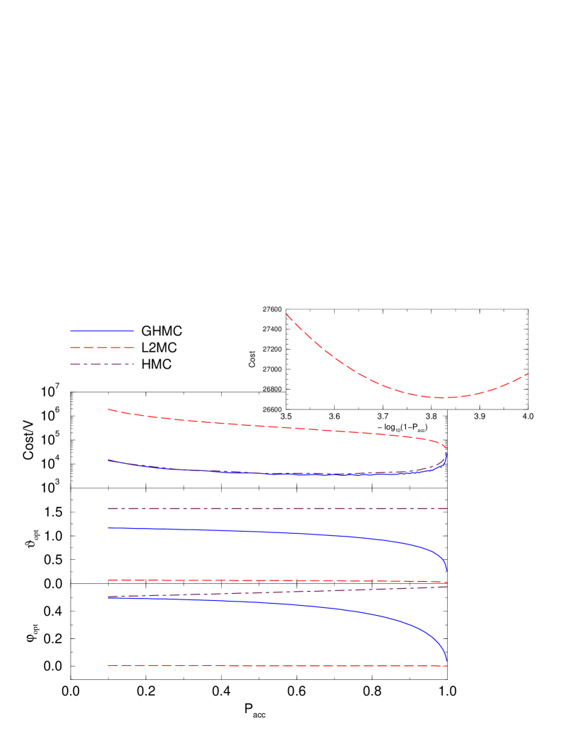
Figure 2: Cost as a function of average Metropolis acceptance rate for the GHMC algorithm compared to HMC and L2MC for free field theory using the lowest order leapfrog integration scheme. The operator under consideration is the “magnetic susceptibility”, i.e., the connected quadratic operator depending only on the lowest frequency mode. The corresponding parameters, the momentum mixing angle ${{\vartheta}_{\hbox{\rm\tiny opt}}}$ and the average trajectory length measured as a fraction of the correlation length ${{\varphi}_{\hbox{\rm\tiny opt}}}={{\tau}_{\hbox{\rm\tiny opt}}}/\xi$ are also shown, all as a function of the acceptance rate ${{\bar{P}}_{\hbox{\rm\tiny acc}}}$. The inset graph shows the region where the acceptance rate is very close to unity which is where the L2MC algorithm has its minimum cost.

8.2.2 HMC

The Hybrid Monte Carlo algorithm corresponds to setting $\vartheta=\pi/2$, and thus we find that the optimal trajectory length in this case is ${{\varphi}_{\hbox{\rm\tiny opt}}}=1/\sqrt{4-{{\bar{P}}_{\hbox{\rm\tiny acc}}}}$, corresponding to a cost

$${{{\twelvefk C}}_{\hbox{\rm\tiny opt}}}={2V\sqrt{4-{{\bar{P}}_{\hbox{\rm\tiny acc}}}}\over{{\bar{P}}_{\hbox{\rm\tiny acc}}}{\delta\tau}m}.$$

This is also shown in Figure 2.

8.3 Fixed Length Trajectories

For fixed length trajectories we shall only analyse the case of L2MC for which the trajectory length $\varphi=m{\delta\tau}$. In this case ${{c}_{\hbox{\rm\tiny opt}}}$ satisfies

$$\frac{{{\bar{P}}_{\hbox{\rm\tiny acc}}}{{c}_{\hbox{\rm\tiny opt}}}^{2}(\cos{{\varphi}_{\hbox{\rm\tiny opt}}})^{2}+3{{c}_{\hbox{\rm\tiny opt}}}^{2}{{\bar{P}}_{\hbox{\rm\tiny acc}}}+{{\bar{P}}_{\hbox{\rm\tiny acc}}}(\cos{{\varphi}_{\hbox{\rm\tiny opt}}})^{2}-{{\bar{P}}_{\hbox{\rm\tiny acc}}}-2{{c}_{\hbox{\rm\tiny opt}}}^{2}-4{{c}_{\hbox{\rm\tiny opt}}}{{\bar{P}}_{\hbox{\rm\tiny acc}}}(\cos{{\varphi}_{\hbox{\rm\tiny opt}}})^{2}+2}{{{\bar{P}}_{\hbox{\rm\tiny acc}}}\left({{{c}_{\hbox{\rm\tiny opt}}}}^{2}(\cos{{\varphi}_{\hbox{\rm\tiny opt}}})^{2}-{{c}_{\hbox{\rm\tiny opt}}}^{2}-(\cos{{\varphi}_{\hbox{\rm\tiny opt}}})^{2}+1\right)}=0.$$

This, together with the corresponding cost, is also plotted in Figure 2. From this figure it is clear that the minimum cost occurs for ${{\bar{P}}_{\hbox{\rm\tiny acc}}}$ very close to unity, where the scaling variable $x=V{\delta\tau}^{6}$ is very small. We may then express ${{c}_{\hbox{\rm\tiny opt}}}$ as

$${{c}_{\hbox{\rm\tiny opt}}}=1-m\left(x\over V\right)^{1/6}+{\mathchoice{\textstyle{1\over 2}}{\scriptstyle{1\over 2}}{\scriptscriptstyle{1\over 2}}{1/2}}m^{2}\left(x\over V\right)^{1/3}-{11\over 24}m^{3}\left(x\over V\right)^{1/2}+\ldots,$$

and likewise

$${{\bar{P}}_{\hbox{\rm\tiny acc}}}=1-\sqrt{5\over 8\pi}\left(1+{9m^{2}\over 20}+{39m^{4}\over 800}+O(m^{6})\right)\sqrt{x}+O(x^{3/2}).$$

From these relations we find that the minimum cost for L2MC is

$${{{\twelvefk C}}_{\hbox{\rm\tiny opt}}}=2\left(10\over\pi\right)^{1/4}V^{5/4}m^{-3/2}.$$

This result tells us that not only does the tuned L2MC algorithm have a dynamical critical exponent $z=3/2$, but also it has a volume dependence of exactly the same form as HMC. We may understand why this behaviour occurs rather than the naive [14] $V^{7/6}m^{-1}$ by the following simple argument.

If ${{\bar{P}}_{\hbox{\rm\tiny acc}}}<1$ then the system will carry out a random walk backwards and forwards along a trajectory because the momentum, and thus the direction of travel, must be reversed upon a Metropolis rejection. A simple minded analysis is that the average time between rejections must be $O(1/m)$ in order to achieve $z=1$. This time is approximately

$$\sum_{n=0}^{\infty}{{\bar{P}}_{\hbox{\rm\tiny acc}}}^{n}(1-{{\bar{P}}_{\hbox{\rm\tiny acc}}})n{\delta\tau}={{{\bar{P}}_{\hbox{\rm\tiny acc}}}{\delta\tau}\over 1-{{\bar{P}}_{\hbox{\rm\tiny acc}}}}={1\over m}.$$

For small ${\delta\tau}$ we have $1-{{\bar{P}}_{\hbox{\rm\tiny acc}}}=\mathop{\rm erf}\sqrt{kV{\delta\tau}^{6}}\propto\sqrt{V{\delta\tau}^{6}}$ where $k$ is a constant, and hence we must scale ${\delta\tau}$ so as to keep $V{\delta\tau}^{4}/m^{2}$ fixed. Since the L2MC algorithm has a naive dynamical critical exponent $z=1$, this means that the cost should vary as ${\twelvefk C}\propto V(V{\delta\tau}^{4}m^{-2})^{1/4}/m{\delta\tau}=V^{5/4}m^{-3/2}$.

9 Autocorrelations and Frequency of Measurement

In this final section we perform an elementary analysis of the general problem of determining the optimal frequency for making measurements of observables on a Markov chain.

Suppose we wish to measure the expectation value $\langle\Omega\rangle$ of an operator $\Omega$ by means of a Markov process (not necessarily HMC). If the cost of making one Markov step is ${\twelvefk C}_{S}$, and the cost of making one measurement of $\Omega$ is ${\twelvefk C}_{M}$, how often should we make measurements in order to minimise the cost of the calculation? Due to the presence of correlations between successive measurements, the answer is not quite trivial.

Consider a sequence of $N_{u}$ uncorrelated measurements of $\Omega$. The sample variance $\bar{V}^{u}_{\Omega}$ is related to the intrinsic variance $V_{\Omega}$ in the distribution of $\Omega$ in the usual way

$$\bar{V}^{u}_{\Omega}\equiv\left\langle\left(\bar{\Omega}-\langle\bar{\Omega}\rangle\right)^{2}\right\rangle={\left\langle\left(\Omega-\langle\Omega\rangle\right)^{2}\right\rangle\over N_{u}}\equiv{V^{u}_{\Omega}\over N_{u}}.$$ (75)

For the general case of $N_{c}$ successive correlated measurements, from equation (36), the sample variance $\bar{V}_{\Omega}$ is

$$\bar{V}^{u}_{\Omega}\equiv\left\langle\left(\bar{\Omega}-\langle\bar{\Omega}\rangle\right)^{2}\right\rangle=(1+2A_{\Omega})\ {\left\langle\left(\Omega-\langle\Omega\rangle\right)^{2}\right\rangle\over N_{c}}=(1+2A_{\Omega})\ {V_{\Omega}\over N_{c}}$$ (76)

so that on average $1+2A_{\Omega}$ correlated measurements are needed to reduce the variance by the same amount as a single truly independent measurement. If the cost of measuring $\Omega$ is small (large), then it should be beneficial to make more (less) than one measurement per decorrelation time.

Let $T$ be the total number of Markov steps required to generate one independent sample, and let $K$ be the number of Markov steps between each measurement of $\Omega$, so that the number of measurements performed per independent sample is $T/K$. If we wish to make sufficient measurements to generate $N$ independent samples, from equations (75) and (76) we have

$$\frac{1+2A_{K}}{T/K}=1,$$ (77)

where $A_{K}$ is the integrated autocorrelation function for measurements separated by $K$ Markov steps. The total cost ${\twelvefk C}$ of the entire process (steps plus measurements) is clearly

$${\twelvefk C}=N\left({\twelvefk C}_{S}T+{\twelvefk C}_{M}\frac{T}{K}\right).$$ (78)

Eliminating $T$ from equations (77) and (78) we obtain

$${\twelvefk C}=N\left({\twelvefk C}_{S}+\frac{{\twelvefk C}_{M}}{K}\right)\left(1+2A_{K}\right)K.$$

The integrated autocorrelation function $A_{K}$ can be written in terms of the autocorrelation function $C_{\Omega}(Kl)$ of section (6.1). Assuming equation (35) we have

$$A_{K}=\sum_{l=1}^{\infty}C_{\Omega}(Kl)=\sum_{l=1}^{\infty}e^{-Kl/{{N}_{\hbox{\rm\tiny exp}}}}=\frac{1}{e^{K/{{N}_{\hbox{\rm\tiny exp}}}}-1}$$

and so

$${\twelvefk C}=\left(K{\twelvefk C}_{S}+{\twelvefk C}_{M}\right)\left(\frac{e^{K/{{N}_{\hbox{\rm\tiny exp}}}}+1}{e^{K/{{N}_{\hbox{\rm\tiny exp}}}}-1}\right)\,.$$

Minimising with respect to $K$ gives

$${\rm sinh}x=x+\alpha$$ (79)

where

$$x\equiv\frac{K}{{{N}_{\hbox{\rm\tiny exp}}}}\qquad\mbox{and}\qquad\alpha\equiv\frac{{\twelvefk C}_{M}}{K{\twelvefk C}_{S}}.$$

For small $\alpha$ where measurements are “cheap” we find

$$K_{\rm opt}={{N}_{\hbox{\rm\tiny exp}}}\left(\frac{6{\twelvefk C}_{M}}{{\twelvefk C}_{S}{{N}_{\hbox{\rm\tiny exp}}}}\right)^{1/3},$$

while for large $\alpha$ where they are “expensive”, we obtain

$$K_{\rm opt}={{N}_{\hbox{\rm\tiny exp}}}\ln\left(\frac{2{\twelvefk C}_{M}}{{\twelvefk C}_{S}{{N}_{\hbox{\rm\tiny exp}}}}\right),$$

the slow logarithmic increase of $K_{\rm opt}$ being due to the exponential decay in the autocorrelation function $C_{\Omega}(l)$. The crossover point, $K=1$, occurs when $\alpha\approx 0.1752$.

10 Conclusions

We have introduced some powerful techniques for analysing a wide class of algorithms for free field theory. Whereas inventing algorithms which are efficacious for free field theory but useless for interesting ones is a popular but fruitless exercise, the analysis of generic algorithms for free fields is apparently very informative. The reason that this is so is because our algorithms are sufficiently dumb that they spent most of their time in dealing with the trivial almost free “modes” of the system.

As evidence of the more general applicability of our analysis we point to the excellent agreement with empirical Monte Carlo data of the $\mathop{\rm erfc}$ form for the Metropolis acceptance probability as a function of integration step size [25, 26]. Futhermore preliminary results for simple models [5] indicate that their autocorrelations have at least the same form as expected from our free field theory results.

Perhaps the most surprising result is the failure of the L2MC (Kramers) algorithm to have superior performance to the HMC algorithm. Despite the fact that the noise is put into the Markov process more smoothly the desirable properties of the L2MC algorithm are upset by its “Zitterbewegung” caused by its rare Metropolis rejections.

It is also somewhat unexpected that the HMC algorithm performs nearly as well as the full GHMC algorithm, of which it is a special case, when the parameters of both are chosen optimally. The broad minimum of the costs of these algorithms as a function of acceptance rate has the pleasant consequence that no very fine tuning of parameters is required.

The result that the optimal HMC trajectory length is about the same as the correlation length of the underlying field theory is significant, in that it indicates that the temptation to use shorter, and hence cheaper, trajectories for systems near criticality should be avoided.

The results pertaining to higher order (Campostrini) integrators [22, 23] are of theoretical interest, but in practice they do not seem to be very useful because the trajectories for interacting field theories are chaotic [27, 28] and apparently limited by the intrinsic instability of the integrators [12].

Appendix A Inverse Laplace Transforms
for Autocorrelation Functions

A.1 Exponentially-Distributed Trajectory Lengths

In this case the Laplace transform of the autocorrelation function, $F(\beta)={\cal L}C(t)$, is a rational function with the numerator of lower degree than the denominator. If the denominator is square free then we have the partial fraction expansion

$$F=\sum_{k}{A_{k}\over\beta-B_{k}}.$$

Since

$${\cal L}e^{-\alpha t}\equiv\int_{0}^{\infty}dt\,e^{-\beta t}e^{-\alpha t}={1\over\alpha+\beta}\qquad(\mathop{\rm Re}\alpha+\beta>0),$$

we have

$${\cal L}^{-1}F=\sum_{k}A_{k}e^{B_{k}t}.$$

The roots $B_{k}$ of the denominator of $F$ come in complex conjugate pairs because the coefficients in $F$ are real. The autocorrelation function can therefore always be written as a sum of real exponentials (corresponding to the real roots) and of real exponentials multiplied by cosines (corresponding to pairs of complex conjugate roots).

If the denominator of $F$ is not square free then the repeated roots give terms of the form $A/(\beta-B)^{n}$ in the partial fraction expansion. Consider then

$${\cal L}t^{n-1}e^{-\alpha t}\equiv\int_{0}^{\infty}dt\,e^{-\beta t}t^{n-1}e^{-\alpha t}=(\alpha+\beta)^{-n}\Gamma(n)\qquad(\mathop{\rm Re}\alpha+\beta>0),$$

This serves to give the inverse Laplace transform in the general case.

A.2 Fixed Length Trajectories

Here $F$ is a rational function of $\zeta\equiv e^{-\beta\tau}$ with the numerator being of lower or equal degree than the denominator. For simplicity we first consider the case where the denominator is square free, whence by partial fractions

$$F=C+\sum_{k}{A_{k}\over\zeta-B_{k}}.$$

Observe that

$${\cal L}\delta(t)\equiv\int_{0}^{\infty}e^{-\beta t}\delta(t)=1,$$

and, more generally,

$${\cal L}\sum_{j=0}^{\infty}\mu^{j}\delta(t-\tau j)=\sum_{j=0}^{\infty}\mu^{j}e^{-\beta\tau j}={1\over 1-\mu e^{-\beta\tau}}\qquad(|\mu|<1),$$

so we have

$${\cal L}^{-1}F = C\delta(t)-\sum_{k}{A_{k}\over B_{k}}\sum_{j=0}^{\infty}B_{k}^{-j}\delta(t-\tau j)$$

$$= C\delta(t)-\sum_{k}A_{k}\sum_{j=0}^{\infty}e^{-(j+1)\ln B_{k}}\delta(t-\tau j).$$

All the the roots must satisfy $|B_{k}|>1$ for the geometric series to converge at $\beta=0\quad(\zeta=1)$, which is necessary for the integrated autocorrelation function $F(0)$ to be finite.

In the general case where the denominator of $F$ has multiple roots the general form of the inverse Laplace transform may be obtained from the identity

$${\cal L}\sum_{j=0}^{\infty}{n+j-1\choose j}\mu^{j}\delta(t-\tau j)=(1-\mu\zeta)^{-n}\qquad(|\mu\zeta|<1).$$

A.3 Example of Computation of Autocorrelation Function

To illustrate the computation of autocorrelation functions we shall explicitly evaluate the connected autocorrelation function for $M^{2}$ for the HMC algorithm with exponentially distributed trajectory lengths. The Laplace transform of the autocorrelation function is

$$F(\beta)={\frac{{{r}}^{3}+2\,{{r}}^{2}\beta+{r}\,{\beta}^{2}+2\,{{m}}^{2}{r}}{{\beta}^{3}+2\,{r}\,{\beta}^{2}+\left({{r}}^{2}+4\,{{m}}^{2}\right)\beta+2\,{{m}}^{2}{r}}}.$$

If we write this in terms of two distinct roots $\beta_{1}$ and $\beta_{2}$ of the denominator

$$F(\beta)={\frac{{r}\,\left({{r}}^{2}+2\,{r}\,\beta+{\beta}^{2}+2\,{{m}}^{2}\right)}{\left(\beta-\beta_{{1}}\right)\left(\beta-\beta_{{2}}\right)\left(2\,{r}+\beta_{{1}}+\beta_{{2}}+\beta\right)}}$$

we can expand this in terms of partial fractions to give

$$F(\beta) = {\frac{{r}\,\left(2\,{{r}}^{4}+4\,{{r}}^{3}\beta_{{1}}+\left(2\,{\beta_{{1}}}^{2}-{{m}}^{2}\right){{r}}^{2}+\beta_{{1}}{r}\,{{m}}^{2}+32\,{{m}}^{4}+4\,{\beta_{{1}}}^{2}{{m}}^{2}\right)}{\left(\beta-\beta_{{1}}\right)\left(2\,{{r}}^{4}-13\,{{m}}^{2}{{r}}^{2}+64\,{{m}}^{4}\right)}}$$

$$+ {\frac{{r}\,\left(\begin{array}[]{c}-4\,{{r}}^{3}\beta_{{1}}+\left(-2\,{\beta_{{1}}}^{2}-13\,{{m}}^{2}-2\,\beta_{{2}}\beta_{{1}}\right){{r}}^{2}\\ +\left(-7\,\beta_{{2}}-8\,\beta_{{1}}\right){{m}}^{2}{r}+16\,{{m}}^{4}+\left(-4\,{\beta_{{1}}}^{2}-4\,\beta_{{2}}\beta_{{1}}\right){{m}}^{2}\end{array}\right)}{\left(\beta-\beta_{{2}}\right)\left(2\,{{r}}^{4}-13\,{{m}}^{2}{{r}}^{2}+64\,{{m}}^{4}\right)}}$$

$$+ {\frac{{r}\,\left(\left(2\,\beta_{{2}}\beta_{{1}}+{{m}}^{2}\right){{r}}^{2}+\left(7\,\beta_{{2}}+7\,\beta_{{1}}\right){{m}}^{2}{r}+16\,{{m}}^{4}+4\,\beta_{{2}}\beta_{{1}}{{m}}^{2}\right)}{\left(2\,{r}+\beta_{{1}}+\beta_{{2}}+\beta\right)\left(2\,{{r}}^{4}-13\,{{m}}^{2}{{r}}^{2}+64\,{{m}}^{4}\right)}}.$$

The inverse Laplace transform of this is immediately obvious

$${\frac{{r}\,\left(2\,{{r}}^{4}+4\,{{r}}^{3}\beta_{{1}}+\left(2\,{\beta_{{1}}}^{2}-{{m}}^{2}\right){{r}}^{2}+\beta_{{1}}{r}\,{{m}}^{2}+32\,{{m}}^{4}+4\,{\beta_{{1}}}^{2}{{m}}^{2}\right){e^{\beta_{{1}}t}}}{2\,{{r}}^{4}-13\,{{m}}^{2}{{r}}^{2}+64\,{{m}}^{4}}}$$

$$+{\frac{{r}\,\left(\begin{array}[]{c}-4\,{{r}}^{3}\beta_{{1}}+\left(-2\,{\beta_{{1}}}^{2}-13\,{{m}}^{2}-2\,\beta_{{2}}\beta_{{1}}\right){{r}}^{2}\\ +\left(-7\,\beta_{{2}}-8\,\beta_{{1}}\right){{m}}^{2}{r}+16\,{{m}}^{4}+\left(-4\,{\beta_{{1}}}^{2}-4\,\beta_{{2}}\beta_{{1}}\right){{m}}^{2}\end{array}\right){e^{\beta_{{2}}t}}}{2\,{{r}}^{4}-13\,{{m}}^{2}{{r}}^{2}+64\,{{m}}^{4}}}$$

$$+{\frac{{r}\,\left(\begin{array}[]{c}\left(2\,\beta_{{2}}\beta_{{1}}+{{m}}^{2}\right){{r}}^{2}+\left(7\,\beta_{{2}}+7\,\beta_{{1}}\right){{m}}^{2}{r}\\ +16\,{{m}}^{4}+4\,\beta_{{2}}\beta_{{1}}{{m}}^{2}\end{array}\right){e^{-\left(2\,{r}+\beta_{{1}}+\beta_{{2}}\right)t}}}{2\,{{r}}^{4}-13\,{{m}}^{2}{{r}}^{2}+64\,{{m}}^{4}}}.$$

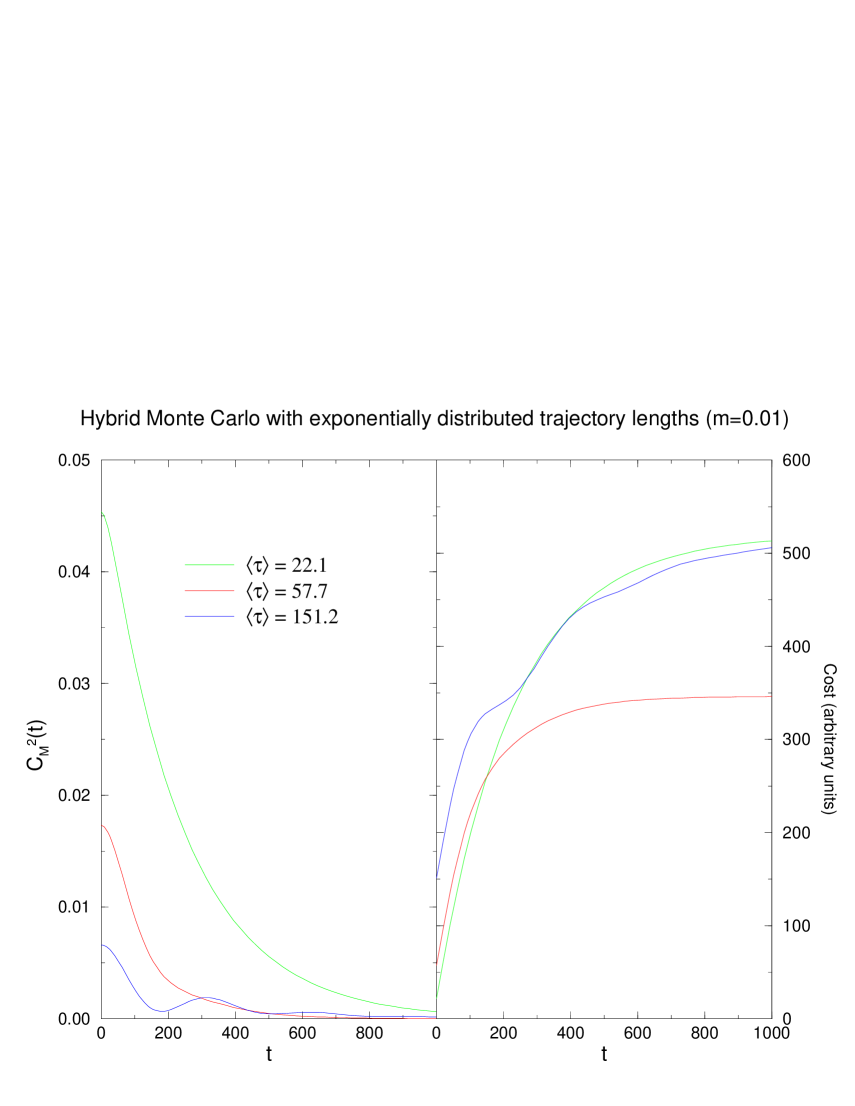
Figure 3: The autocorrelation function and the cumulative cost are shown as functions of MD time for the optimal trajectory length and those costing 50% more.

In figure 3 we show this function for $m=10^{-2}$ and the optimal value ${{r}_{\hbox{\rm\tiny opt}}}=\sqrt{3}m$, together with the two neighbouring values of $r=(3\sqrt{3}\pm\sqrt{15})m/2$ for which the cost is 50% greater.

Appendix B Evaluation of Spectral Averages

In this section we show how to evaluate the following spectral sums for one-dimensional free field theory:

$$\sigma_{A}^{(\alpha)} \equiv {1\over V}\sum_{p\in{\twelvebb Z}_{V}}\sin^{2\alpha}\left({\pi p\over V}\right)$$ (83)

$$= {1\over 2^{2\alpha}}\left\{{2\alpha\choose\alpha}+\sum_{k=1}^{\lfloor\alpha/V\rfloor}(-)^{kV}\left[{2\alpha\choose\alpha-kV}+{2\alpha\choose\alpha+kV}\right]\right\},$$ (84)

$$\sigma_{m^{2}}^{(\alpha)} \equiv {1\over V}\sum_{p\in{\twelvebb Z}_{V}}\omega_{p}^{2\alpha}$$ (85)

$$= \sum_{\beta=0}^{\alpha}{\alpha\choose\beta}m^{2(\alpha-\beta)}\left\{{2\beta\choose\beta}+2\sum_{k=1}^{\lfloor\beta/V\rfloor}(-)^{kV}{2\beta\choose\beta-kV}\right\},$$ (86)

$$\tilde{\sigma}_{m^{2}} \equiv {1\over V}\sum_{p\in{\twelvebb Z}_{V}}\cos(2\tau\omega_{p})$$ (87)

$$= \sum_{\beta=0}^{\infty}{(-2m^{2})^{\beta}\over\beta!}\left(\prod_{\gamma=0}^{\beta-1}\tau_{\gamma}\int^{\tau_{\gamma}}d\tau_{\gamma+1}\right)\sum_{k\in{\twelvebb Z}}{\mathop{\rm J_{2kV}}}(4\tau),$$ (88)

$$\bar{\sigma}_{m^{2}}^{(\alpha)} \equiv {1\over V}\sum_{p\in{\twelvebb Z}_{V}}\omega_{p}^{2\alpha}\sin^{2}(\tau\omega_{p})$$ (89)

$$= {1\over 2}\sigma_{m^{2}}^{(\alpha)}-{1\over 2}\left(-{1\over 4}{d^{2}\over d\tau^{2}}\right)^{\alpha}\tilde{\sigma}_{m^{2}},$$ (90)

where

$$\omega_{p}^{2}\equiv m^{2}+4\sin^{2}\left({\pi p\over V}\right).$$ (91)

B.1 Completeness relations

Let ${\cal G}$ be a group with a family of $D$-dimensional representations $\phi_{q}:{\cal G}\to({\twelvebb C}^{D}\to{\twelvebb C}^{D})$, i.e., $\phi_{q}(g):{\twelvebb C}^{D}\to{\twelvebb C}^{D}$, labelled by some parameter $q$; thus $\phi_{q}(gh)=\phi_{q}(g)\phi_{q}(h)$ for $g,h\in{\cal G}$. Summing over group elements (or integrating with respect to Haar measure in the continuous case) gives

$$\sigma_{q}\equiv\int_{\cal G}d\mu\,\phi_{q}(g),$$

and multiplying by $\phi_{q}(h)$ for any $h\in{\cal G}$ we find

$$\phi_{q}(h)\sigma_{q} = \phi_{q}(h)\int_{\cal G}d\mu\,\phi_{q}(g)=\int_{\cal G}d\mu\,\phi_{q}(h)\phi_{q}(g)$$

$$= \int_{\cal G}d\mu\,\phi_{q}(hg)=\int_{\cal G}d\mu\,\phi_{q}(g^{\prime})=\sigma_{q}$$

where we have made use of the (left) invariance of Haar measure $d\mu$. Hence either $\phi_{q}(h)=1\quad\forall h\in{\cal G}$ or $\sigma_{q}=0$. If we let $q=0$ label the identity representation of ${\cal G}$, and all other $\phi_{q}$ be non-identity representations, we have

$$\sigma_{q}=\delta(q).$$

Example B.1.1

Let ${\cal G}={\twelvebb Z}_{V}$, $q\in{\twelvebb Z}_{V}$, and $\phi_{q}(p)=e^{2\pi ipq/V}$:

$${1\over V}\sum_{p\in{\twelvebb Z}_{V}}e^{2\pi ipq/V}=\delta_{q,0};$$

Example B.1.2

Let ${\cal G}={\twelvebb Z}$, $q\in{\twelvebb S}_{1}=[0,2\pi]$, and $\phi_{q}(p)=e^{ipq}$:

$${1\over 2\pi}\sum_{p\in{\twelvebb Z}}e^{ipq}=\delta(q);$$

Example B.1.3

Let ${\cal G}={\twelvebb S}_{1}$, $q\in{\twelvebb Z}$, and $\phi_{q}(p)=e^{ipq}$:

$${1\over 2\pi}\int_{0}^{2\pi}dp\,e^{ipq}=\delta_{q,0}.$$

B.2 A Poisson Resummation Formula

Let $f:{\twelvebb S}_{1}\to{\twelvebb S}_{1}$ be a periodic function. As it is periodic it obviously wants to be expanded in eigenfunctions of ${\twelvebb S}_{1}$:

$$f(p) = \int_{0}^{2\pi}dp^{\prime}\,\delta(p^{\prime}-p)f(p^{\prime})\qquad[p\in{\twelvebb S}_{1}]$$

$$= \int_{0}^{2\pi}dp^{\prime}\,{1\over 2\pi}\sum_{q\in{\twelvebb Z}}e^{iq(p^{\prime}-p)}f(p^{\prime})$$

$$= \sum_{q\in{\twelvebb Z}}e^{-iqp}{1\over 2\pi}\int_{0}^{2\pi}dp^{\prime}\,e^{iqp^{\prime}}f(p^{\prime}),$$

hence the “spectral average”

$$\sigma(f) = {1\over V}\sum_{p\in{\twelvebb Z}_{V}}f\left({2\pi p\over V}\right)$$

$$= {1\over V}\sum_{p\in{\twelvebb Z}_{V}}\sum_{q\in{\twelvebb Z}}e^{-2\pi ipq/V}{1\over 2\pi}\int_{0}^{2\pi}dp^{\prime}\,e^{iqp^{\prime}}f(p^{\prime})$$

$$= \sum_{q\in{\twelvebb Z}}\Biggl{\{}{1\over V}\sum_{p\in{\twelvebb Z}_{V}}e^{-2\pi ipq/V}\Biggr{\}}\Biggl{\{}{1\over 2\pi}\int_{0}^{2\pi}dp^{\prime}\,e^{iqp^{\prime}}f(p^{\prime})\Biggr{\}}$$

$$= \sum_{q\in{\twelvebb Z}}\Biggl{\{}\sum_{k\in{\twelvebb Z}}\delta_{q,kV}\Biggr{\}}\Biggl{\{}{1\over 2\pi}\int_{0}^{2\pi}dp^{\prime}\,e^{iqp^{\prime}}f(p^{\prime})\Biggr{\}}$$

$$= \sum_{k\in{\twelvebb Z}}{1\over 2\pi}\int_{0}^{2\pi}dp^{\prime}\,e^{ip^{\prime}kV}f(p^{\prime}).$$

As $f$ is real valued we may take the real part of this identity to obtain

$$\sigma(f)\equiv{1\over V}\sum_{p\in{\twelvebb Z}_{V}}f\left({2\pi p\over V}\right)=\sum_{k\in{\twelvebb Z}}{1\over 2\pi}\int_{0}^{2\pi}dp^{\prime}\,\cos(p^{\prime}kV)f(p^{\prime}).$$ (92)

B.3 Multiple Angle Expansion

The following simple identity is often useful

$$\sin^{2\alpha}\theta = \left[{1\over 2i}\left(e^{i\theta}-e^{-i\theta}\right)\right]^{2\alpha}\qquad(\alpha\in{\twelvebb N})$$ (93)

$$= \left({1\over 2i}\right)^{2\alpha}\sum_{q=0}^{2\alpha}{2\alpha\choose q}(-)^{q}e^{2i(\alpha-q)\theta}$$

$$= \left({1\over 2i}\right)^{2\alpha}\left\{{2\alpha\choose\alpha}(-)^{\alpha}+\sum_{q=0}^{\alpha-1}{2\alpha\choose q}(-)^{q}2\cos[2(\alpha-q)\theta]\right\}$$

$$= {1\over 2^{2\alpha}}\left\{{2\alpha\choose\alpha}+\sum_{q^{\prime}=1}^{\alpha}{2\alpha\choose\alpha-q^{\prime}}(-)^{q^{\prime}}2\cos(2q^{\prime}\theta)\right\}.$$

B.4 Free-field Spectral Sums

Let us first consider equation (83). From equation (92) we have

$${1\over V}\sum_{p\in{\twelvebb Z}_{V}}\cos\left({2\pi pq^{\prime}\over V}\right)=\sum_{k\in{\twelvebb Z}}{1\over 2\pi}\int_{0}^{2\pi}dp^{\prime}\,\cos(p^{\prime}kV)\cos(p^{\prime}q^{\prime})$$

$$\qquad=\sum_{k_{i}n{\twelvebb Z}}{1\over 2\pi}\int_{0}^{2\pi}{1\over 2}\Bigl{\{}\cos[p^{\prime}(kV+q^{\prime})]+\cos[p^{\prime}(kV-q^{\prime})]\Bigr{\}}$$

$$\qquad=\sum_{k\in{\twelvebb Z}}{1\over 2}\Bigl{\{}\delta_{kV+q^{\prime},0}+\delta_{kV-q^{\prime},0}\Bigr{\}}.$$

Using the multiple-angle expansion (93) we obtain

$$\sigma_{A}^{(\alpha)} \equiv {1\over V}\sum_{p\in{\twelvebb Z}_{V}}\sin^{2\alpha}\left({\pi p\over V}\right)$$

$$= {1\over V}\sum_{p\in{\twelvebb Z}_{V}}{1\over 2^{2\alpha}}\left\{{2\alpha\choose\alpha}+\sum_{q^{\prime}=1}^{\alpha}{2\alpha\choose\alpha-q^{\prime}}(-)^{q^{\prime}}2\cos\left({2\pi pq^{\prime}\over V}\right)\right\}$$

$$= {1\over 2^{2\alpha}}\left\{{2\alpha\choose\alpha}+\sum_{q^{\prime}=1}^{\alpha}{2\alpha\choose\alpha-q^{\prime}}(-)^{q^{\prime}}{2\over V}\sum_{p\in{\twelvebb Z}_{V}}\cos\left({2\pi pq^{\prime}\over V}\right)\right\}$$

$$= {1\over 2^{2\alpha}}\left\{{2\alpha\choose\alpha}+\sum_{q^{\prime}=1}^{\alpha}{2\alpha\choose\alpha-q^{\prime}}(-)^{q^{\prime}}\sum_{k\in{\twelvebb Z}}\left(\delta_{kV+q^{\prime},0}+\delta_{kV-q^{\prime},0}\right)\right\}$$

$$= {1\over 2^{2\alpha}}\left\{{2\alpha\choose\alpha}+\sum_{k=1}^{\lfloor\alpha/V\rfloor}(-)^{kV}\left[{2\alpha\choose\alpha-kV}+{2\alpha\choose\alpha+kV}\right]\right\}.$$

From this result we may obtain an expression for the quantity $\sigma_{m^{2}}^{(\alpha)}$ defined in equation (85)

$$\sigma_{m^{2}}^{(\alpha)} \equiv {1\over V}\sum_{p\in{\twelvebb Z}_{V}}\omega_{p}^{2\alpha}={1\over V}\sum_{p\in{\twelvebb Z}_{V}}\left[m^{2}+4\sin^{2}\left({\pi p\over V}\right)\right]^{\alpha}$$

$$= \sum_{\beta=0}^{\alpha}{\alpha\choose\beta}{1\over V}\sum_{p\in{\twelvebb Z}_{V}}m^{2(\alpha-\beta)}4^{\beta}\sin^{2\beta}\left({\pi p\over V}\right)$$

$$= \sum_{\beta=0}^{\alpha}{\alpha\choose\beta}m^{2(\alpha-\beta)}4^{\beta}\sigma_{A}^{(\beta)}$$

$$= \sum_{\beta=0}^{\alpha}{\alpha\choose\beta}m^{2(\alpha-\beta)}\left\{{2\beta\choose\beta}+2\sum_{k=1}^{\lfloor\beta/V\rfloor}(-)^{kV}{2\beta\choose\beta-kV}\right\}.$$

Example B.4.1

$$\sigma_{m^{2}}^{(2)}={1\over V}\sum_{p\in{\twelvebb Z}_{V}}\omega_{p}^{4}=\left(6+4m^{2}+m^{4}\right)+\delta_{V,1}\left(-6-4m^{2}\right)+\delta_{V,2}\cdot 2;$$

Example B.4.2

$$\sigma_{m^{2}}^{(3)} = {1\over V}\sum_{p\in{\twelvebb Z}_{V}}\omega_{p}^{6}=\left(m^{6}+6m^{4}+18m^{2}+20\right)$$

$$\qquad+\delta_{V,1}\left(-6m^{4}-18m^{2}-20\right)+\delta_{V,2}\left(6m^{2}+12\right)-\delta_{V,3}\cdot 2.$$

In order to evaluate Equation (87) we first investigate the simpler case where $m=0$

$$\tilde{\sigma}_{0} \equiv {1\over V}\sum_{p\in{\twelvebb Z}_{V}}\cos(2\tau\omega_{p})$$

$$= \sum_{k\in{\twelvebb Z}}{1\over 2\pi}\int_{0}^{2\pi}dp^{\prime}\,\cos(p^{\prime}kV)\cos\left[4\tau\sin\left({p^{\prime}\over 2}\right)\right]$$

$$= \sum_{k\in{\twelvebb Z}}{1\over\pi}\int_{0}^{\pi}d\theta\,\cos(2kV\theta)\cos[4\tau\sin\theta]$$

$$= \sum_{k\in{\twelvebb Z}}{\mathop{\rm J_{2kV}}}(4\tau).$$

For small $m$ we Taylor expand $\tilde{\sigma}_{m^{2}}$

$$\tilde{\sigma}_{m^{2}}=\sum_{\beta=0}^{\infty}{m^{2\beta}\over\beta!}\left.{d^{\beta}\tilde{\sigma}_{m^{2}}\over d(m^{2})^{\beta}}\right|_{m^{2}=0}.$$

Consider the quantity

$$-{1\over 2}{d\over dm^{2}}{d\over d\tau}{\tilde{\sigma}_{m^{2}}\over\tau} = -{1\over 2}{d\over d\tau}\left({1\over\tau}{d\over dm^{2}}{1\over V}\sum_{p\in{\twelvebb Z}_{V}}\cos(2\tau\omega_{p})\right)$$

$$= {d\over d\tau}\left({1\over\tau}{1\over V}\sum_{p\in{\twelvebb Z}_{V}}\sin(2\tau\omega_{p})\tau{d\omega_{p}\over dm^{2}}\right)$$

$$= {d\over d\tau}\left({1\over V}\sum_{p\in{\twelvebb Z}_{V}}\sin(2\tau\omega_{p}){1\over 2\omega_{p}}\right)$$

$$= {1\over V}\sum_{p\in{\twelvebb Z}_{V}}\cos(2\tau\omega_{p})=\tilde{\sigma}_{m^{2}};$$

upon integrating with respect to $\tau$ we obtain

$${d\tilde{\sigma}_{m^{2}}\over dm^{2}}=-2\tau\int^{\tau}d\tau^{\prime}\,\tilde{\sigma}_{m^{2}},$$

and hence

$$\left.{d^{\beta}\tilde{\sigma}_{m^{2}}\over d(m^{2})^{\beta}}\right|_{m^{2}=0}=(-2)^{\beta}\tau\int^{\tau}d\tau_{1}\,\tau_{1}\int^{\tau_{1}}d\tau_{2}\ldots\tau_{\beta-1}\int^{\tau_{\beta-1}}\,d\tau_{\beta}\tilde{\sigma}_{0}.$$

By this means we have obtained the desired result

$$\tilde{\sigma}_{m^{2}}=\sum_{\beta=0}^{\infty}{(-2m^{2})^{\beta}\over\beta!}\left(\prod_{\gamma=0}^{\beta-1}\tau_{\gamma}\int^{\tau_{\gamma}}d\tau_{\gamma+1}\right)\tilde{\sigma}_{0}.$$

Equation (89) may be found by differentiating $\tilde{\sigma}_{m^{2}}$ with respect to $\tau$,

$$\bar{\sigma}_{m^{2}}^{(\alpha)} \equiv {1\over V}\sum_{p\in{\twelvebb Z}_{V}}\omega_{p}^{2\alpha}\sin^{2}(\tau\omega_{p})$$

$$= {1\over 2V}\sum_{p\in{\twelvebb Z}_{V}}\omega_{p}^{2\alpha}\Bigl{\{}1-\cos(2\tau\omega_{p})\Bigr{\}}$$

$$= {1\over 2}\sigma_{m^{2}}^{(\alpha)}-{1\over 2}\left(-{1\over 4}{d^{2}\over d\tau^{2}}\right)^{\alpha}\tilde{\sigma}_{m^{2}}.$$

Example B.4.3

$$\bar{\sigma}_{m^{2}}^{(2)} = {1\over V}\sum_{p\in{\twelvebb Z}_{V}}\omega_{p}^{4}\sin^{2}(\tau\omega_{p})$$ (94)

$$= {1\over 2}\sigma_{m^{2}}^{(2)}-{1\over 2}\sum_{\beta=0}^{\infty}{m^{2\beta}\over\beta!}\left(-{1\over 4}{d^{2}\over d\tau^{2}}\right)^{2}\left.{d^{\beta}\tilde{\sigma}_{m^{2}}\over d(m^{2})^{\beta}}\right|_{m^{2}=0}$$

$$= {1\over 2}\sigma_{m^{2}}^{(2)}-\sum_{k\in{\twelvebb Z}}\sum_{\beta=0}^{\infty}{(-2m^{2})^{\beta}\over 2\beta!}\left(-{1\over 4}{d^{2}\over d\tau^{2}}\right)^{2}\times$$

$$\qquad\qquad\qquad\times\left(\prod_{\gamma=0}^{\beta-1}\tau_{\gamma}\int^{\tau_{\gamma}}d\tau_{\gamma+1}\right){\mathop{\rm J_{2kV}}}(4\tau).$$

The $\beta=0$ term in the sum is

$$-{1\over 2}\sum_{k\in{\twelvebb Z}}\left(-{1\over 4}{d^{2}\over d\tau^{2}}\right)^{2}{\mathop{\rm J_{2kV}}}(4\tau)=-8\sum_{k\in{\twelvebb Z}}{\mathop{\rm J_{2kV}}}^{\prime\prime\prime\prime}(4\tau).$$

From the recurrence relation

$${\mathop{\rm J_{n}}}^{\prime}={1\over 2}({\mathop{\rm J_{n-1}}}-{\mathop{\rm J_{n+1}}})$$

we find that

$${d^{k}{\mathop{\rm J_{n}}}(z)\over dz^{k}}={1\over 2^{k}}\sum_{\gamma=0}^{k}{k\choose\gamma}(-)^{\gamma}{\mathop{\rm J_{n-k+2\gamma}}}(z),$$

which we may prove by induction:

$${d^{k+1}{\mathop{\rm J_{n}}}(z)\over dz^{k+1}}={1\over 2^{k}}\sum_{\gamma=0}^{k}{k\choose\gamma}(-)^{\gamma}{d{\mathop{\rm J_{n-k+2\gamma}}}(z)\over dz}$$

$$\qquad={1\over 2^{k+1}}\sum_{\gamma=0}^{k}{k\choose\gamma}(-)^{\gamma}\Bigl{(}{\mathop{\rm J_{n-k+2\gamma-1}}}(z)-{\mathop{\rm J_{n-k+2\gamma+1}}}(z)\Bigr{)}$$

$$\qquad={1\over 2^{k+1}}\sum_{\gamma=0}^{k}{k\choose\gamma}(-)^{\gamma}\Bigl{(}{\mathop{\rm J_{n-(k+1)+2\gamma}}}(z)-{\mathop{\rm J_{n-(k+1)+2(\gamma+1)}}}(z)\Bigr{)}$$

$$\qquad={1\over 2^{k+1}}\Biggl{\{}\sum_{\gamma=1}^{k}\left[{k\choose\gamma}+{k\choose\gamma-1}\right](-)^{\gamma}{\mathop{\rm J_{n-(k+1)+2\gamma}}}(z)+$$

$$\qquad\qquad\qquad\qquad+{\mathop{\rm J_{n-(k=1)}}}(z)-{\mathop{\rm J_{n+(k+1)}}}(z)\Biggr{\}}$$

$$\qquad={1\over 2^{k+1}}\sum_{\gamma=0}^{k+1}{k+1\choose\gamma}(-)^{\gamma}{\mathop{\rm J_{n-(k+1)+2\gamma}}}(z),$$

using ${k\choose\gamma}+{k\choose\gamma-1}={k+1\choose\gamma}$. We therefore find that

$$-8\sum_{k\in{\twelvebb Z}}{\mathop{\rm J_{2kV}}}^{\prime\prime\prime\prime}(4\tau)=-2\sum_{k\in{\twelvebb Z}}\sum_{\gamma=0}^{4}{4\choose\gamma}(-)^{\gamma}{\mathop{\rm J_{2kV-4+2\gamma}}}(4\tau)$$

$$\qquad=-2\sum_{k\in{\twelvebb Z}}\Bigl{\{}{\mathop{\rm J_{2kV-4}}}(4\tau)-4{\mathop{\rm J_{2kV-2}}}(4\tau)+$$

$$\qquad\qquad\qquad+6{\mathop{\rm J_{2kV}}}(4\tau)-4{\mathop{\rm J_{2kV+2}}}(4\tau)+{\mathop{\rm J_{2kV+4}}}(4\tau)\Bigr{\}}$$

$$\qquad=-3{\mathop{\rm J_{0}}}(4\tau)+4{\mathop{\rm J_{2}}}(4\tau)-{\mathop{\rm J_{4}}}(4\tau)-$$

$$\qquad\qquad\qquad-2\sum_{k=1}^{\infty}\Bigl{\{}{\mathop{\rm J_{2kV-4}}}(4\tau)-4{\mathop{\rm J_{2kV-2}}}(4\tau)+$$

$$\qquad\qquad\qquad\qquad+6{\mathop{\rm J_{2kV}}}(4\tau)-4{\mathop{\rm J_{2kV+2}}}(4\tau)+{\mathop{\rm J_{2kV+4}}}(4\tau)\Bigr{\}}.$$

The $\beta=1$ term in the sum (94) is

$$-{1\over 2}\sum_{k\in{\twelvebb Z}}-2m^{2}\left(-{1\over 4}{d^{2}\over d\tau^{2}}\right)^{2}\tau\int^{\tau}d\tau_{1}\,{\mathop{\rm J_{2kV}}}(4\tau_{1})$$

$$\qquad=m^{2}\sum_{k\in{\twelvebb Z}}{d^{4}\over d\hat{\tau}^{4}}\cdot\hat{\tau}\int^{\hat{\tau}}d\tau^{\prime}\,{\mathop{\rm J_{2kV}}}(\tau^{\prime})\qquad({\rm where\ }\hat{\tau}\equiv 4\tau)$$

$$\qquad=m^{2}\sum_{k\in{\twelvebb Z}}{d^{3}\over d\hat{\tau}^{3}}\left\{\int^{\hat{\tau}}d\tau^{\prime}\,{\mathop{\rm J_{2kV}}}(\tau^{\prime})+\hat{\tau}{\mathop{\rm J_{2kV}}}(\hat{\tau})\right\}$$

$$\qquad=m^{2}\sum_{k\in{\twelvebb Z}}\Bigl{\{}4{\mathop{\rm J_{2kV}}}^{\prime\prime}(\hat{\tau})+\hat{\tau}{\mathop{\rm J_{2kV}}}^{\prime\prime\prime}(\hat{\tau})\Bigr{\}}$$

$$\qquad=m^{2}\sum_{k\in{\twelvebb Z}}\Biggl{\{}\sum_{\gamma=0}^{2}{2\choose\gamma}(-)^{\gamma}{\mathop{\rm J_{2kV-2+2\gamma}}}(\hat{\tau})+$$

$$\qquad\qquad\qquad+{\hat{\tau}\over 8}\sum_{\gamma=0}^{3}{3\choose\gamma}(-)^{\gamma}{\mathop{\rm J_{2kV-3+2\gamma}}}(\hat{\tau})\Biggr{\}}$$

$$\qquad=m^{2}\sum_{k\in{\twelvebb Z}}\Bigl{\{}{\mathop{\rm J_{2kV-2}}}(\hat{\tau})-2{\mathop{\rm J_{2kV}}}(\hat{\tau})+{\mathop{\rm J_{2kV+2}}}(\hat{\tau})+$$

$$\qquad\qquad+{\hat{\tau}\over 8}{\mathop{\rm J_{2kV-3}}}(\hat{\tau})-{3\hat{\tau}\over 8}{\mathop{\rm J_{2kV-1}}}(\hat{\tau})+{3\hat{\tau}\over 8}{\mathop{\rm J_{2kV+1}}}(\hat{\tau})-{\hat{\tau}\over 8}{\mathop{\rm J_{2kV+3}}}(\hat{\tau})\Bigr{\}}$$

$$\qquad=m^{2}\Biggl{\{}-2{\mathop{\rm J_{0}}}(4\tau)+2{\mathop{\rm J_{2}}}(4\tau)+3\tau{\mathop{\rm J_{1}}}(4\tau)-\tau{\mathop{\rm J_{3}}}(4\tau)+$$

$$\qquad\qquad+\sum_{k=1}^{\infty}\bigl{(}2{\mathop{\rm J_{2kV-2}}}(4\tau)-4{\mathop{\rm J_{2kV}}}(4\tau)+2{\mathop{\rm J_{2kV+2}}}(4\tau)+$$

$$\qquad\qquad\qquad+\tau{\mathop{\rm J_{2kV-3}}}(4\tau)-3\tau{\mathop{\rm J_{2kV-1}}}(4\tau)+$$

$$\qquad\qquad\qquad+3\tau{\mathop{\rm J_{2kV+1}}}(4\tau)-\tau{\mathop{\rm J_{2kV+3}}}(4\tau)\bigr{)}\Biggr{\}}.$$

B.5 Results for Campostrini

$$\bar{\sigma}^{(4)}_{m^{2}} = \Bigl{[}35-35{\mathop{\rm J_{0}}}(4\tau)+56{\mathop{\rm J_{2}}}(4\tau)-28{\mathop{\rm J_{4}}}(4\tau)+8{\mathop{\rm J_{6}}}(4\tau)-{\mathop{\rm J_{8}}}(4\tau)\Bigr{]}$$

$$+ \Bigl{[}40-40{\mathop{\rm J_{0}}}(4\tau)+64t{\mathop{\rm J_{1}}}(4\tau)+31{\mathop{\rm J_{2}}}(4\tau)-8{\mathop{\rm J_{4}}}(4\tau)+{\mathop{\rm J_{6}}}(4\tau)\Bigr{]}m^{2}$$

$$+ \Bigl{[}18+(16t^{2}-18){\mathop{\rm J_{0}}}(4\tau)+48t{\mathop{\rm J_{1}}}(4\tau)+8{\mathop{\rm J_{2}}}(4\tau)-{\mathop{\rm J_{4}}}(4\tau)\Bigr{]}m^{4}+O(m^{6}),$$

$$\bar{\sigma}^{(6)}_{m^{2}} = \left[\begin{array}[]{c}462-462{\mathop{\rm J_{0}}}(4\tau)+792{\mathop{\rm J_{2}}}(4\tau)-495{\mathop{\rm J_{4}}}(4\tau)\\ +220{\mathop{\rm J_{6}}}(4\tau)-66{\mathop{\rm J_{8}}}(4\tau)+12{\mathop{\rm J_{10}}}(4\tau)-{\mathop{\rm J_{12}}}(4\tau)\end{array}\right]$$

$$+ \left[\begin{array}[]{c}756-756{\mathop{\rm J_{0}}}(4\tau)+1024t{\mathop{\rm J_{1}}}(4\tau)+698{\mathop{\rm J_{2}}}(4\tau)\\ -256{\mathop{\rm J_{4}}}(4\tau)+69{\mathop{\rm J_{6}}}(4\tau)-12{\mathop{\rm J_{8}}}(4\tau)+{\mathop{\rm J_{10}}}(4\tau)\end{array}\right]m^{2}$$

$$+ \left[\begin{array}[]{c}525+(256t^{2}-525){\mathop{\rm J_{0}}}(4\tau)+1152t{\mathop{\rm J_{1}}}(4\tau)\\ +316{\mathop{\rm J_{2}}}(4\tau)-74{\mathop{\rm J_{4}}}(4\tau)+12{\mathop{\rm J_{6}}}(4\tau)-{\mathop{\rm J_{8}}}(4\tau)\end{array}\right]m^{4}+O(m^{6}),$$

$$\bar{\sigma}^{(8)}_{m^{2}} = \left[\begin{array}[]{c}6435-6435{\mathop{\rm J_{0}}}(4\tau)+11440{\mathop{\rm J_{2}}}(4\tau)-8008{\mathop{\rm J_{4}}}(4\tau)\\ +4368{\mathop{\rm J_{6}}}(4\tau)-1820{\mathop{\rm J_{8}}}(4\tau)+560{\mathop{\rm J_{10}}}(4\tau)\\ -120{\mathop{\rm J_{12}}}(4\tau)+16{\mathop{\rm J_{14}}}(4\tau)-{\mathop{\rm J_{16}}}(4\tau)\end{array}\right]$$

$$+ \left[\begin{array}[]{c}13728-13728{\mathop{\rm J_{0}}}(4\tau)+16384t{\mathop{\rm J_{1}}}(4\tau)\\ +14075{\mathop{\rm J_{2}}}(4\tau)-6128{\mathop{\rm J_{4}}}(4\tau)+2185{\mathop{\rm J_{6}}}(4\tau)\\ -608{\mathop{\rm J_{8}}}(4\tau)+123{\mathop{\rm J_{10}}}(4\tau)-16{\mathop{\rm J_{12}}}(4\tau)+{\mathop{\rm J_{14}}}(4\tau)\end{array}\right]m^{2}$$

$$+ \left[\begin{array}[]{c}12936+(4096t^{2}-12936){\mathop{\rm J_{0}}}(4\tau)\\ +24576t{\mathop{\rm J_{1}}}(4\tau)+9280{\mathop{\rm J_{2}}}(4\tau)-2807{\mathop{\rm J_{4}}}(4\tau)\\ +688{\mathop{\rm J_{6}}}(4\tau)-128{\mathop{\rm J_{8}}}(4\tau)+16{\mathop{\rm J_{10}}}(4\tau)-{\mathop{\rm J_{12}}}(4\tau)\end{array}\right]m^{4}+O(m^{6}),$$

$$\bar{\sigma}^{(10)}_{m^{2}} = \left[\begin{array}[]{c}92378-92378{\mathop{\rm J_{0}}}(4\tau)+167960{\mathop{\rm J_{2}}}(4\tau)\\ -125970{\mathop{\rm J_{4}}}(4\tau)+77520{\mathop{\rm J_{6}}}(4\tau)-38760{\mathop{\rm J_{8}}}(4\tau)\\ +15504{\mathop{\rm J_{10}}}(4\tau)-4845{\mathop{\rm J_{12}}}(4\tau)+1140{\mathop{\rm J_{14}}}(4\tau)\\ -190{\mathop{\rm J_{16}}}(4\tau)+20{\mathop{\rm J_{18}}}(4\tau)-{\mathop{\rm J_{20}}}(4\tau)\end{array}\right]$$

$$+ \left[\begin{array}[]{c}243100-243100{\mathop{\rm J_{0}}}(4\tau)+262144t{\mathop{\rm J_{1}}}(4\tau)\\ +267814{\mathop{\rm J_{2}}}(4\tau)-129872{\mathop{\rm J_{4}}}(4\tau)+54252{\mathop{\rm J_{6}}}(4\tau)\\ -19024{\mathop{\rm J_{8}}}(4\tau)+5420{\mathop{\rm J_{10}}}(4\tau)-1200{\mathop{\rm J_{12}}}(4\tau)\\ +193{\mathop{\rm J_{14}}}(4\tau)-20{\mathop{\rm J_{16}}}(4\tau)+{\mathop{\rm J_{18}}}(4\tau)\end{array}\right]m^{2}$$

$$+ \left[\begin{array}[]{c}289575+(65536t^{2}-289575){\mathop{\rm J_{0}}}(4\tau)\\ +491520t{\mathop{\rm J_{1}}}(4\tau)+233612{\mathop{\rm J_{2}}}(4\tau)-82714{\mathop{\rm J_{4}}}(4\tau)\\ +25164{\mathop{\rm J_{6}}}(4\tau)-6392{\mathop{\rm J_{8}}}(4\tau)+1300{\mathop{\rm J_{10}}}(4\tau)\\ -198{\mathop{\rm J_{12}}}(4\tau)+20{\mathop{\rm J_{14}}}(4\tau)-{\mathop{\rm J_{16}}}(4\tau)\end{array}\right]m^{4}+O(m^{6}).$$

Appendix C Spectral sum for one dimensional free field theory

We wish to evaluate the spectral sum

$$\sigma^{(-1)}_{m^{2}}\equiv{1\over V}\sum_{p\in{\twelvebb Z}_{V}}\omega_{p}^{-2}$$

for large $V$. Using the Poisson resummation formula we obtain

$$\sigma^{(-1)}_{m^{2}}=\sum_{k\in{\twelvebb Z}}{1\over 2\pi}\int_{0}^{2\pi}dp^{\prime}\,\cos(p^{\prime}kV)\,\omega_{Vp^{\prime}/2\pi}^{-2}=\sum_{k\in{\twelvebb Z}}{1\over 2\pi}\int_{0}^{2\pi}dp^{\prime}\,{\cos(p^{\prime}kV)\over m^{2}+4\sin^{2}({\mathchoice{\textstyle{1\over 2}}{\scriptstyle{1\over 2}}{\scriptscriptstyle{1\over 2}}{1/2}}p^{\prime})}.$$

Upon substituting $z\equiv e^{ip^{\prime}}$ we get

$$\sigma^{(-1)}_{m^{2}} = \sum_{k\in{\twelvebb Z}}{i\over 4\pi}\oint_{|z|=1}dz\,{z^{kV}+z^{-kV}\over z^{2}-(m^{2}+2)z+1}$$

$$= \sum_{k\in{\twelvebb Z}}{i\over 2\pi}\oint_{|z|=1}dz\,{z^{|k|V}\over(z-\mu_{+})(z-\mu_{-})}={1\over m\sqrt{m^{2}+4}}\left[{1+\mu_{-}^{V}\over 1-\mu_{-}^{V}}\right],$$

where $\mu_{\pm}\equiv 1+{\mathchoice{\textstyle{1\over 2}}{\scriptstyle{1\over 2}}{\scriptscriptstyle{1\over 2}}{1/2}}m^{2}\pm{\mathchoice{\textstyle{1\over 2}}{\scriptstyle{1\over 2}}{\scriptscriptstyle{1\over 2}}{1/2}}m\sqrt{m^{2}+4}$. For $m\ll 1$ we have $\mu_{-}=1-m+O(m^{2})$, and thus

$$\sigma^{(-1)}_{m^{2}}={\coth{{\mathchoice{\textstyle{1\over 2}}{\scriptstyle{1\over 2}}{\scriptscriptstyle{1\over 2}}{1/2}}mV}\over m\sqrt{m^{2}+4}}$$

which is correct to all orders in the large $V$ asymptotic expansion.

Appendix D Spectral sum for two dimensional free field theory

We want to evaluate the spectral sum

$$\sigma\equiv{1\over L_{x}L_{y}}\sum_{p_{x}\in{\twelvebb Z}_{L_{x}}\atop p_{y}\in{\twelvebb Z}_{L_{y}}}\omega_{p}^{-2}$$

where

$$\omega_{p}^{2}\equiv m^{2}+4\left(\sin^{2}{p_{x}\pi\over L_{x}}+\sin^{2}{p_{y}\pi\over L_{y}}\right).$$

Using Poisson resummation we find that for $L_{x},L_{y}\to\infty$

$$\sigma={1\over(2\pi)^{2}}\int_{0}^{2\pi}dp^{\prime}_{x}\,dp^{\prime}_{y}\,\left[m^{2}+4\left(\sin^{2}{p^{\prime}_{x}\over 2}+\sin^{2}{p^{\prime}_{y}\over 2}\right)\right]^{-1},$$

so upon substituting $z\equiv e^{ip^{\prime}_{x}}$ we obtain

$$\sigma = {i\over 4\pi^{2}}\int_{0}^{2\pi}dp^{\prime}_{y}\oint_{|z|=1}{dz\over z^{2}-\Bigl{(}m^{2}+4\sin^{2}({\mathchoice{\textstyle{1\over 2}}{\scriptstyle{1\over 2}}{\scriptscriptstyle{1\over 2}}{1/2}}p^{\prime}_{y})\Bigr{)}z+1}$$

$$= {i\over 4\pi^{2}}\int_{0}^{2\pi}dp^{\prime}_{y}\oint_{|z|=1}{dz\over(z-\mu)(z-1/\mu)}$$

where

$$\mu\equiv{m^{2}\over 2}+2\sin^{2}{p^{\prime}_{y}\over 2}+1-\sqrt{\left({m^{2}\over 2}+2\sin^{2}{p^{\prime}_{y}\over 2}+1\right)^{2}-1}.$$

Evaluating the contour integral gives

$$\sigma=-{1\over 2\pi}\int_{0}^{2\pi}dp^{\prime}_{y}\,\left(\mu-{1\over\mu}\right)^{-1}={1\over 4\pi}\int_{0}^{2\pi}dp^{\prime}_{y}\,\left[\left({m^{2}\over 2}+2\sin^{2}{p^{\prime}_{y}\over 2}+1\right)^{2}-1\right]^{-{\mathchoice{\textstyle{1\over 2}}{\scriptstyle{1\over 2}}{\scriptscriptstyle{1\over 2}}{1/2}}}.$$

We now make the substitution $z^{\prime}\equiv e^{ip^{\prime}_{y}}$, which leads to

$$\sigma = -{i\over 2\pi}\oint_{|z^{\prime}|=1}{dz^{\prime}\over\sqrt{\left[(m^{2}+4)z^{\prime}-z^{\prime 2}-1\right]^{2}-4z^{\prime 2}}}$$

$$= -{i\over 2\pi}\oint_{|z^{\prime}|=1}{dz^{\prime}\over\sqrt{\left[z^{\prime 2}-(m^{2}+2)z^{\prime}+1\right]\left[z^{\prime 2}-(m^{2}+6)z^{\prime}+1\right]}}$$

$$= -{i\over 2\pi}\oint_{|z^{\prime}|=1}{dz^{\prime}\over\sqrt{(z^{\prime}-a)(z^{\prime}-1/a)(z^{\prime}-b)(z^{\prime}-1/b)}},$$

where

$$a \equiv {m^{2}\over 2}+3-\sqrt{\left({m^{2}\over 2}+3\right)^{2}-1}=(3-2\sqrt{2})-{1\over 8}(3\sqrt{2}-4)m^{2}+\cdots$$

$$b \equiv {m^{2}\over 2}+1-\sqrt{\left({m^{2}\over 2}+1\right)^{2}-1}=1-m+{\mathchoice{\textstyle{1\over 2}}{\scriptstyle{1\over 2}}{\scriptscriptstyle{1\over 2}}{1/2}}m^{2}+\cdots.$$

Since $1/a>1/b>1>b>a>0$ the contour integral may be shrunk to be the integral along the branch cut from $a$ to $b$,

$$\sigma={1\over\pi}\int_{a}^{b}{dz^{\prime}\over\sqrt{(z^{\prime}-a)(b-z^{\prime})(1/a-z^{\prime})(1/b-z^{\prime})}}.$$

If we change variables to

$$x\equiv{(a+1)(z^{\prime}-1)\over(a-1)(z^{\prime}+1)}$$

we obtain

$$\sigma=-{2\sqrt{ab}\over\pi(a+1)(b-1)}\int_{1}^{1/k^{\prime}}{dx\over\sqrt{(x^{2}-1)(1-k^{\prime 2}x^{2})}}$$

where $k^{\prime}\equiv{(a-1)(b+1)\over(a+1)(b-1)}$. With the substitution $\xi\equiv{1\over k}\sqrt{1-{1\over x^{2}}}$ we find that

$$\int_{1}^{1/k^{\prime}}{dx\over\sqrt{(x^{2}-1)(1-k^{\prime 2}x^{2})}}=\int_{0}^{1}{d\xi\over\sqrt{(1-\xi^{2})(1-k^{2}\xi^{2})}}=K(k)$$

where $K$ is the complete elliptic integral and $k^{2}+k^{\prime 2}=1$; thus

$$\sigma=-{2\sqrt{ab}\over\pi(a+1)(b-1)}K(k).$$

This may be further simplified using Landen’s transformation

$$K\left(2\sqrt{\eta}\over 1+\eta\right)=(1+\eta)K(\eta)$$

with $\eta\equiv{a-b\over 1-ab}$, which leads to

$$\sigma={2\sqrt{ab}\over\pi(1-ab)}K\left({b-a\over 1-ab}\right),$$

using the fact that $K$ is an even function. Expanding in powers of $m$ we obtain

$$\sigma={1\over\pi}\Bigl{(}1+O(m)\Bigr{)}K\Bigl{(}1-\sqrt{2}m+O(m^{2})\Bigr{)}={1\over 4\pi}\ln\left({32\over m^{2}}\right)+O(m\ln m),$$

because

$$K(k)=K(\sqrt{1-k^{\prime 2}})\sim\ln{4\over k^{\prime}}\qquad\mbox{as $k^{\prime}\to 0$}.$$

References

- [1] Simon Duane, A. D. Kennedy, Brian J. Pendleton, and Duncan Roweth. Hybrid Monte Carlo. Phys. Lett., 195B(2):216–222, 1987.
- [2] A. D. Kennedy. The theory of Hybrid Stochastic algorithms. In P. H. Damgaard et al., editors, Probabilistic Methods in Quantum Field Theory and Quantum Gravity, pages 209–223, New York, 1990. NATO, Plenum Press. Lectures given at the workshop on “Probabilistic Methods in Quantum Field Theory and Quantum Gravity,” Cargése, August 1989.
- [3] A. D. Kennedy and Brian J. Pendleton. Acceptances and autocorrelations in Hybrid Monte Carlo. In Urs M. Heller, A. D. Kennedy, and Sergiu Sanielevici, editors, Lattice ’90, volume B20 of Nuclear Physics (Proceedings Supplements), pages 118–121, 1991. Talk presented at “Lattice ’90,” Tallahassee.
- [4] A. D. Kennedy. Hybrid Monte Carlo algorithm on the Connection Machine. Intl. J. Mod. Phys., C3:1–26, 1992.
- [5] A. D. Kennedy, Robert G. Edwards, Hidetoshi Mino, and Brian J. Pendleton. Tuning the generalized Hybrid Monte Carlo algorithm. In Tien D. Kieu, Bruce H. J. McKellar, and Anthony J. Guttmann, editors, Lattice ’95, volume B47 of Nuclear Physics (Proceedings Supplements), pages 781–784, 1995, hep-lat/9509043. Proceedings of the 13th International Symposium on Lattice Field Theory, Melbourne, Australia, 11–15 July 1995.
- [6] A. D. Kennedy and Brian Pendleton. Cost of generalised HMC algorithms for free field theory. In M. Campostrini, S. Caracciolo, L. Cosmai, A. DiGiacomo, F. Rapuano, and P. Rossi, editors, Lattice ’99, volume B83–84 of Nuclear Physics (Proceedings Supplements), pages 816–818, 1999, hep-lat/0001031. Proceedings of the XVIIth International Symposium on Lattice Field Theory, Pisa, Italy, 29 June–3 July 1999.
- [7] A. D. Kennedy. The Hybrid Monte Carlo algorithm on parallel computers. Parallel Computing, 25:1311–1339, 1999.
- [8] A. D. Kennedy. Monte carlo methods for quantum field theory. Chinese Journal of Physics, 2000. To be published.
- [9] Robert G. Edwards, Ivan Horváth, and A. D. Kennedy. Non-reversibility of molecular dynamics trajectories. In Bernard et al. [29], pages 971–973, hep-lat/9608020. Proceedings of the XIVth International Symposium on Lattice Field Theory, St. Louis, Missouri, 4–8 June 1996.
- [10] Robert G. Edwards, Ivan Horváth, and A. D. Kennedy. Instabilities and non-reversibility of molecular dynamics trajectories. Nucl. Phys., B484:375–399, 1997, hep-lat/9606004.
- [11] Ivan Horváth and A. D. Kennedy. The Local Hybrid Monte Carlo algorithm for free field theory: Reexamining overrelaxation. Nucl. Phys., B510:367–400, 1998, hep-lat/9708024.
- [12] Balint Joo, Brian Pendleton, Anthony D. Kennedy, Alan C. Irving, James C. Sexton, Stephen M. Pickles, and Stephen P. Booth (UKQCD Collaboration). Instability in the Molecular Dynamics step of Hybrid Monte Carlo in dynamical fermion lattice QCD simulations. 2000, hep-lat/0005023.
- [13] A. D. Kennedy, Julius Kuti, Steffen Meyer, and Brian J. Pendleton. Program for efficient Monte Carlo computations of quenched lattice gauge theory using the quasi-heatbath method on a CDC CYBER 205 computer. J. Comp. Phys, 64:133–160, 1986.
- [14] Alan M. Horowitz. A generalized guided Monte Carlo algorithm. Phys. Lett., B268:247–252, 1991.
- [15] Matteo Beccaria and Giuseppe Curci. The Kramers equation simulation algorithm. 1. operator analysis. Phys. Rev., D49:2578–2589, 1994, hep-lat/9307007.
- [16] O. Klein. Arkiv Mat. Astr. Fys., 16(5), 1922.
- [17] Julius Kuti. Lattice field theories and dynamical fermions. In Richard D. Kenway and G. S. Pawley, editors, Computational Physics, pages 311–378. Scottish Universities Summer School in Physics, Scottish Universities Summer School in Physics, 1987.
- [18] Alan Horowitz. Stochastic quantization in phase space. Phys. Lett., 156B:89, 1985.
- [19] Alan Horowitz. The second order Langevin equation and numerical simulations. Nucl. Phys., B280[FS18](3):510–522, March 1987.
- [20] R. T. Scalettar, D. J. Scalapino, and R. L. Sugar. New algorithm for the numerical simulation of fermions. Phys. Rev., B34:7911, 1986.
- [21] Paul B. Mackenzie. An improved Hybrid Monte Carlo method. Phys. Lett., B226:369, 1989.
- [22] Massimo Campostrini and Paolo Rossi. A comparison of numerical algorithms for dynamical fermions. Nucl. Phys., B329:753, 1990.
- [23] Michael Creutz and Andreas Gocksch. Higher order Hybrid Monte Carlo algorithms. Phys. Rev. Lett., 63:9, 1989.
- [24] H. Gausterer and M. Salmhofer. Remarks on global Monte Carlo algorithms. Phys. Rev., D40(8):2723–2726, October 1989.
- [25] Sourendu Gupta, Anders Irbäck, Frithjof Karsch, and Bengt Petersson. The acceptance probability in the Hybrid Monte Carlo method. Phys. Lett., B242:437–443, 1990.
- [26] Balint Joo et al. Parallel tempering in lattice QCD with -improved Wilson fermions. Phys. Rev., D59:114501, 1999, hep-lat/9810032.
- [27] Karl Jansen and Chuan Liu. Study of Liapunov exponents and the reversibility of molecular dynamics algorithms. In Bernard et al. [29], pages 974–976, hep-lat/9607057. Proceedings of the XIVth International Symposium on Lattice Field Theory, St. Louis, Missouri, 4–8 June 1996.
- [28] Khalil M. Bitar, Robert G. Edwards, Urs M. Heller, and A. D. Kennedy. QCD function with two flavours of dynamical Wilson fermions. Phys. Rev., D54:3546–3550, 1996, hep-lat/9602010.
- [29] Claude Bernard, Maarten Golterman, and Michael Ogilvie, editors. volume B53 of Nuclear Physics (Proceedings Supplements), 1997. Proceedings of the XIVth International Symposium on Lattice Field Theory, St. Louis, Missouri, 4–8 June 1996.