Center Vortices and Monopoles without lattice Gribov copies

Abstract

We construct a smooth gauge for the adjoint field which is free of ambiguities on the lattice. In this Laplacian Center Gauge, center vortices and monopoles appear together as local gauge defects. A numerical study of center vortices in $SU(2)$ and $SU(3)$ supports equality of the $Z_{N}$ and $SU(N)$ string tensions in the continuum limit, and only then.

PACS numbers: 11.15.Ha, 12.38.Aw, 12.38.Gc

I Introduction

Ever since the advent of QCD, one has tried to isolate a subset of collective degrees of freedom (d.o.f.) which would be responsible for the non-perturbative features of the $SU(2)$ or $SU(N)$ Yang-Mills theory, in particular for confinement. It is natural to associate non-perturbative effects with topological excitations. Therefore, all the non-trivial homotopy groups $\Pi_{3}(SU(2))={\bf Z}$, $\Pi_{2}(SU(2)/U(1))={\bf Z}$ and $\Pi_{1}(SU(2)/Z_{2})=Z_{2}$, and their $SU(N)$ homologues have been considered. The corresponding topological excitations have codimension 4, 3 and 2 respectively, and are instantons, Abelian monopoles and center vortices. Among these, the latter have been emerging as particularly worthy of attention. Center vortices correspond to non-contractible Wilson loops in the adjoint representation. The simplest example is obtained with an $SU(2)$ gauge field along a Wilson loop of length $L$: $A_{\mu}^{1}=A_{\mu}^{2}=0,A_{\mu}^{3}(x)=2\pi/L$. The Wilson loop $exp(i\oint_{L}dx_{\mu}A_{\mu}^{a}(x)\frac{\sigma^{a}}{2})=exp(i\pi\sigma_{3})$ has trace $exp(2i\pi\sigma_{3})=1$ in the adjoint representation, but is not contractible to the identity.

Numerical lattice simulations have given evidence for the relevant role played by center vortices. Now, topology is a feature of continuum field theory, and studying topological excitations on the lattice requires some kind of interpolation. Non-contractible adjoint loops are rather elusive under direct investigation, so that an indirect approach has been successfully developed [3], in analogy with the detection of Abelian monopoles. Any topological excitation can be exposed as a local gauge-fixing singularity in an otherwise smooth gauge. Abelian monopoles appear as singularities in the Maximal Abelian Gauge, which minimizes the non-Abelian components $\int d^{4}x\sum_{\mu}(|A_{\mu}^{1}(x)|^{2}+|A_{\mu}^{2}(x)|^{2})$. Similarly here, gauge-fixing is used to bring each gauge link as close as possible to a center element, hence the name Maximal Center Gauge. This is equivalent to bringing all adjoint links close to the identity, that is, making the adjoint field as smooth as possible. Each fundamental link matrix $U$ is then decomposed into a part $U^{\prime}\in SU(N)/Z_{N}$, which reproduces the smooth adjoint field and in addition remains close to the $SU(N)$ identity, and a $z\in Z_{N}$ part. The latter seems at first sight irrelevant for the detection of non-contractible adjoint loops. However, such a loop as in the $exp(i\pi\sigma_{3})$ example above, will have a trace in the fundamental representation equal to $-1$, or more generally to a non-trivial $Z_{N}$ element. If one neglects the fluctuations of the $U^{\prime}$ part, center vortices should appear as non-trivial $Z_{N}$ excitations, localized on plaquettes and called $P$-vortices. $P$-vortices form closed co-dimension 2 surfaces in the dual space–time, which disorder the $Z_{N}$ ensemble $\{z\}$. They are localized defects, associated with macroscopic center vortices via gauge-fixing. This indirect strategy, called center projection, has been used to assess numerically the importance of center vortices. Numerical evidence has been accumulating, which shows that this $P$-vortex disorder generates a $Z_{N}$ string tension close in value to the original $SU(N)$ one [3]. A physical density of vortices per ${\rm fm}^{2}$ can be extracted [4]. $SU(N)$ chiral symmetry breaking induces a quark condensate and Dirac zeromodes in the $Z_{N}$ ensemble also [5]. On the other hand, the coset $\{U^{\prime}\}$ ensemble shows no confinement, no chiral symmetry breaking, and no topological charge [6]. While this may be a simple kinematic effect, it is tempting to adhere to the idea of center dominance, according to which center vortices, and nothing else, are responsible for the non-perturbative Yang-Mills features. One implication of center dominance is that the string tension produced by center vortices should match the Yang-Mills string tension exactly.

However, this construction rests on shaky ground. The connection between $Z_{N}$ excitations which are located on a plaquette and their $SU(N)$ ancestors, center vortices believed to be of macroscopic size – smooth examples of which have been explicitly constructed [7] – proceeds via gauge fixing. When each adjoint link is maximally close to the identity, the assignment of a $Z_{N}$ center element to the fundamental link, i.e. the center projection itself, can be performed with the most confidence. However, the technical difficulty of fixing a smooth gauge on the lattice is well known. Gauge fixing proceeds by iterative local maximization of a gauge functional, and this procedure terminates when a local maximum is reached, without any guarantee, or in fact any reasonable hope, of reaching the global maximum. Which local maximum is reached depends on the starting point along the gauge orbit. The various gauges reached correspond to “lattice Gribov copies”. This technical problem, which plagues the Landau and Coulomb gauges on the lattice, is commonly believed to be rather harmless there. In Maximal Center Gauge, its harmful effects have been exhibited [8]: the copy obtained when starting the gauge-fixing procedure from Landau gauge corresponds to a very high value of the gauge-fixing functional, higher than a typical local maximum, but gives, after center projection, $Z_{N}$ excitations which do not confine. Evidence has been produced that, the higher the value of the local maximum one reaches, the smaller the $Z_{N}$ string tension [9]. Although this evidence is currently under dispute [10], the technical problem of lattice Gribov copies prevents a reasonable degree of confidence in the idea of center dominance.

The present paper, we believe, should restore full confidence in this idea. Here, we address and solve the problem of the gauge ambiguity. This problem was already solved for the Landau gauge in Ref.[11]. There, a different gauge was proposed, the Laplacian gauge, which is Lorentz-symmetric and produces a smooth gauge field like the Landau gauge, but has no lattice Gribov copies. The advantages of such an unambiguous gauge have barely been explored [12, 13]. In the present paper, we generalize the construction of [11] to $SU(N)$ in the adjoint representation, since we want the adjoint field to be smooth. In our “Laplacian Center Gauge”, the adjoint $SU(N)/Z_{N}$ field is uniquely gauge-fixed – aside from exceptional configurations which are genuine Gribov copies–, and a remaining local $Z_{N}$ gauge freedom subsists. Now, even though the adjoint field is uniquely gauge-fixed in general, there exists a sub-manifold of points where the gauge remains ill-defined. These local gauge ambiguities are the necessary companions of macroscopic topological excitations. As explained earlier, a non-contractible adjoint Wilson loop will prevent the adjoint field from being smooth everywhere; similarly, an Abelian monopole will correspond to a singularity of the Abelian projected field. Indeed, by studying the details of the gauge condition, we show that on some subset of points the gauge freedom is locally enlarged from $Z_{2}$ to $U(1)$, and from $U(1)$ to $SU(2)$, defining two types of local ambiguities which can be readily identified with center vortices and Abelian monopoles, the latter being embedded in the former, as anticipated in [14, 15]. These topological objects appear naturally together as local gauge defects. This unified description reconciles with center dominance the large body of numerical evidence in favor of monopole dominance: Abelian monopoles do not represent an alternative to center vortices as effective degrees of freedom; they are their undissociable partners. In particular, the condensation of monopoles in the confined phase of the $SU(N)$ theory [16, 17] implies the percolation of center vortex surfaces, by the following simple argument. A non-zero monopole condensate means that a single monopole can be created at point $(x,t)$, or equivalently that monopoles are not pair-wise confined. Since monopole world–lines are closed loops, the monopole at $(x,t)$ must have a partner at $(x^{\prime},t)$, and a “single” monopole simply has a partner at infinity. This in turn means that monopole world–lines percolate. Since we show that monopole world–lines are embedded in center vortex surfaces, percolation of one implies percolation of the other.

We complement the qualitative study of local gauge defects outlined above with a quantitative study, for $SU(2)$ and $SU(3)$. We show that, in Laplacian Center Gauge, the center-projected ensemble confines, while the coset ensemble does not. This confirms earlier $SU(2)$ results [3, 6], and firms up the sketchy $SU(3)$ evidence [18], all obtained in the ambiguous Maximal Center Gauge. But the scenario of center dominance demands exact equality of the $Z_{N}$ and $SU(N)$ string tensions. We test this scenario by considering different Laplacian Center Gauges, obtained from different lattice discretizations of the Laplacian. At finite lattice spacing $a$, different gauges give widely different $Z_{N}$ string tensions, which at first sight looks like a terrible blow to center dominance. Nevertheless, we show that, in all three gauges we consider and presumably in any –unambiguous– gauge, equality of the $Z_{N}$ and $SU(N)$ string tensions is approached as $a\rightarrow 0$. Therefore, our results support the restoration of center dominance in the continuum limit, and only then.

Section II of our paper gives an explicit construction of the Laplacian Center Gauge for $SU(N)$. Section III discusses the local gauge ambiguities and their identification as monopoles and center vortices. Section IV presents our numerical results for $SU(2)$ and $SU(3)$. Section V shows the effect of alternative gauges and discusses center dominance. A final summary and discussion is presented in Section VI.

II Laplacian Center Gauge fixing

The Laplacian gauge was originally proposed by Vink and Wiese [11], who suggested to use the eigenvectors of the covariant Laplacian operator to fix the gauge in a non–Abelian gauge theory: the eigenvectors transform covariantly, and one can fix the gauge by prescribing their color orientation at each space-time point. This method takes advantage of a non–local procedure to fix a covariant smooth gauge in an unambiguous way. There are exceptional cases, genuine Gribov copies, in which the gauge fixed configuration is not unique: however such cases can be easily detected by the presence of degenerate eigenvalues and – from the viewpoint of numerical simulations – never occur. The perturbative formulation of the Laplacian gauge in $SU(2)$ has been studied in [19], while the problem of its renormalizability is still open. Since we are interested in reducing the symmetry of the gauge group from $SU(N)$ to its center $Z_{N}$, it is useful to consider the Laplacian operator in the adjoint representation. In fact, since the adjoint representation is invariant under gauge transformations in $Z_{N}$, the adjoint Laplacian procedure fixes unambiguously the gauge up to the center symmetry, and the Laplacian Center Gauge is just another name for the adjoint Laplacian gauge. The first step towards this construction was already considered, in $SU(2)$, by A. van der Sijs [20].

Consider 4–dimensional lattice $SU(N)$ gauge theory. The adjoint Laplacian operator $\Delta^{ab}_{xy}(\dot{U})$ is given by

$$-\Delta^{ab}_{xy}(\dot{U})=\sum_{\mu}\left(2\,\delta_{x,y}\,\delta^{ab}-\dot{U}_{\mu}^{ab}(x)\,\delta_{y,x+\hat{\mu}}-\dot{U}_{\mu}^{ba}(x-\hat{\mu})\,\delta_{y,x-\hat{\mu}}\right)$$ (1)

where $a$,$b=1,\ldots(N^{2}-1)$ are color indices and $x$,$y$ are space–time lattice coordinates. The dotted $\dot{U}_{\mu}(x)$ are the link variables in the adjoint representation and are related to the links $U_{\mu}(x)$ in the fundamental by

$$\dot{U}_{\mu}^{ab}(x)=\frac{1}{2}\mbox{Tr}\left(\lambda_{a}U_{\mu}(x)\lambda_{b}U_{\mu}^{\dagger}(x)\right)$$ (2)

$\lambda_{i}$, $i=1,\ldots,(N^{2}-1)$ being the generators of $SU(N)$ with the normalization $\mbox{Tr}(\lambda_{a}\lambda_{b})=2\delta_{ab}$. If $V$ is the volume of the lattice, $\Delta(\dot{U})$ is a $[(N^{2}-1)V]\times[(N^{2}-1)V]$ real symmetric matrix which depends on the gauge field. The eigenvalues $\mu_{j}$ of $\Delta$ are real and the eigenvector equation is

$$\Delta^{ab}_{xy}(\dot{U})\phi^{(j)}_{b}(y)=\mu_{j}\,\phi^{(j)}_{a}(x)$$ (3)

where $\phi^{(j)}$, $j=1,\ldots,[(N^{2}-1)V]$ are the $[(N^{2}-1)V]$–dimensional (real) eigenvectors. So we can associate $(N^{2}-1)$–dimensional real vectors $\phi^{(j)}(x)$ to every lattice site.
Let us consider a gauge transformation $U_{\mu}^{\prime}(x)=\Omega(x)U_{\mu}(x)\Omega^{\dagger}(x+\hat{\mu})$ on the fundamental links. Then, making use of the property $\dot{(AB)}=\dot{A}\dot{B}$, the eigenvector equation (3) becomes

$$\dot{\Omega}^{\dagger}\,{}^{ai}(x)\Delta^{ik}_{xy}(\dot{U}^{\prime})\dot{\Omega}^{kb}(y)\phi^{(j)}_{b}(y)=\mu_{j}\,\phi^{(j)}_{a}(x)$$ (4)

This relation shows that the eigenvalues are gauge invariant and the eigenvectors transform according to $\dot{\Omega}^{ab}(x)\phi^{(j)}_{b}(x)=\phi^{(j)}_{a}\,{}^{\prime}(x)$. This transformation law can be rewritten as follows

$$\Omega(x)\Phi^{(j)}(x)\Omega^{\dagger}(x)=\Phi^{(j)}\,{}^{\prime}(x)$$ (5)

where we have defined the $su(N)$ matrices (i.e. in the $SU(N)$ algebra) $\Phi^{(j)}(x)=\sum_{a=1}^{N^{2}-1}\phi^{(j)}_{a}(x)\lambda_{a}$ and $\Phi^{(j)}\,{}^{\prime}(x)=\sum_{a=1}^{N^{2}-1}\phi^{(j)}_{a}\,{}^{\prime}(x)\lambda_{a}$. Gauge transformations rotate the vectors $\phi^{(j)}(x)$ in color space and so we can fix the gauge by requiring a conventional arbitrary orientation for the $\phi^{(j)}(x)$. This orientation may depend on the lattice site and it is fixed once and for all; the simplest choice is to make it space–time independent. We will see below that to perform the reduction of the gauge symmetry from $SU(N)$ to $Z_{N}$ we only need to fix the orientation of two eigenvectors of the Laplacian operator. Since we are interested in fixing a smooth gauge, we consider the two lowest eigenmodes $\phi^{(1)}$ and $\phi^{(2)}$, associated with the smallest eigenvalues of the Laplacian.

The gauge fixing procedure can be split in two steps. In the first, one rotates $\Phi^{(1)}(x)$ at every $x$ so that $\Phi^{(1)}\,{}^{\prime}(x)$ is diagonal, i.e. in the Cartan subalgebra of $su(N)$. This leaves a residual symmetry corresponding to gauge transformations belonging to the Cartan subgroup $U(1)^{N-1}$. Therefore, at that stage we already have obtained an unambiguous Abelian gauge, called Laplacian Abelian Gauge in [20]. Nothing more can be done with only one eigenvector. To further reduce the gauge freedom we must consider a second step where the second eigenvector $\phi^{(2)}$ is taken into account. The gauge transformation that has rotated $\Phi^{(1)}(x)$ to the Cartan subalgebra, maps $\Phi^{(2)}(x)$ to $\Phi^{(2)}\,{}^{\prime}(x)$. While $\Phi^{(1)}\,{}^{\prime}(x)$ is invariant under gauge transformations in $U(1)^{N-1}$, this is in general not the case for $\Phi^{(2)}\,{}^{\prime}(x)$ (special cases are discussed later). The gauge symmetry can now be reduced to $Z_{N}$ by considering gauge transformations in $U(1)^{N-1}$ which make some conventionally chosen color components of the twice rotated matrix $\Phi^{(2)}\,{}^{\prime\prime}(x)$ vanish. The remnant center gauge freedom, consistently with the construction, can not be fixed within the described procedure in the adjoint representation. In fact, as follows from equation (5), the matrices $\Phi^{(j)}(x)$ are invariant under gauge transformations in the center group $Z_{N}$ (these gauge transformations are the identity in the adjoint representation). Now we describe explicitly how to perform the presented two–step program.

Step 1
The starting point is equation (5) for the first eigenvector $\phi^{(1)}$. $\Phi^{(1)}(x)$ is an $N\times N$ (traceless) hermitian matrix, and so there exist $N\times N$ unitary matrices $\Omega(x)$ which diagonalize it (we recall that the diagonal elements are the eigenvalues of $\Phi^{(1)}(x)$). Diagonalizing $\Phi^{(1)}(x)$ is equivalent to requiring that $\Phi^{(1)}\,{}^{\prime}(x)$ be in the Cartan subalgebra of $su(N)$. Since we want $\Omega(x)$ to be a gauge transformation in $SU(N)$, we must require that $\det(\Omega(x))=1$. The condition that $\Phi^{(1)}\,{}^{\prime}(x)$ is diagonal does not specify $\Omega(x)$ – i.e. the gauge symmetry – up to $U(1)^{N-1}$ transformations yet. In fact there are non-diagonal $SU(N)$ gauge transformations which, when applied to $\Phi^{(1)}\,{}^{\prime}(x)$, have the only effect of exchanging the position of the eigenvalues along the diagonal. In order to eliminate this permutation arbitrariness, it is necessary to impose an ordering of the eigenvalues. This is simple to do since the eigenvalues of a hermitian matrix are real. Once some conventional ordering has been chosen, $\Omega(x)$ is really defined up to $U(1)^{N-1}$ transformations. A last remark concerns the explicit evaluation of $\Omega(x)$, which, in view of (5), is the problem of diagonalizing a hermitian matrix. For the $SU(2)$ and $SU(3)$ gauge groups, this evaluation can be performed analytically. For larger groups $SU(N\geq 4)$, one can simply make use of numerical methods.

Step 2
In Step 1 we have found $\Omega(x)$ defined up to gauge transformations $V(x)\in U(1)^{N-1}$. A second step is necessary to reduce the symmetry from $U(1)^{N-1}$ to $Z_{N}$; this means that we must introduce a criterion which specifies $V(x)$ up to $Z_{N}$. Consider the second eigenvector $\phi^{(2)}$ and apply the gauge transformation $\Omega(x)$ to $\Phi^{(2)}(x)$ so as to obtain $\Phi^{(2)}\,{}^{\prime}(x)=\Omega(x)\Phi^{(2)}(x)\Omega^{\dagger}(x)$. Now we look for $V(x)$ such that the vector $\phi^{(2)}\,{}^{\prime\prime}(x)$, obtained from $\Phi^{(2)}\,{}^{\prime\prime}(x)=V(x)\Phi^{(2)}\,{}^{\prime}(x)V^{\dagger}(x)$, has a conventional orientation in color space. Also in this case there is no need that this orientation be the same at all $x$ but, however, this is the simplest choice. In order to make the discussion more transparent, we explicitly consider the $SU(3)$ case; the generalization to $SU(N)$ is straightforward.

A generic matrix $V(x)\in U(1)^{2}$ can be written in the form $V(x)=\mbox{diag}\left(\mbox{e}^{i(2\alpha(x)+\beta(x))},\mbox{e}^{i(-\alpha(x)+\beta(x))},\mbox{e}^{-i(\alpha(x)+2\beta(x))}\right)$ with $\alpha(x)$, $\beta(x)\in[0,2\pi)$. We can fix $V(x)$ up to gauge transformations in $Z_{3}$ by imposing the following requirements:

$$\begin{array}[]{l}\mbox{1) }\mbox{Tr}\left(\Phi^{(2)}\,{}^{\prime\prime}(x)\,\lambda_{2}\right)=0\\ \mbox{2) }\mbox{Tr}\left(\Phi^{(2)}\,{}^{\prime\prime}(x)\,\lambda_{7}\right)=0\\ \mbox{3) }\mbox{Tr}\left(\Phi^{(2)}\,{}^{\prime\prime}(x)\,\lambda_{1}\right)>0,\mbox{Tr}\left(\Phi^{(2)}\,{}^{\prime\prime}(x)\,\lambda_{6}\right)>0\end{array}$$ (6)

The meaning of these three conditions becomes clearer when one writes explicitly $\Phi^{(2)}\,{}^{\prime\prime}(x)$

$$\Phi^{(2)}\,{}^{\prime\prime}(x)=\left(\begin{array}[]{lll}\phi^{(2)}_{3}\,{}^{\prime}+\frac{1}{\sqrt{3}}\phi^{(2)}_{8}\,{}^{\prime}&\left(\phi^{(2)}_{1}\,{}^{\prime}-i\phi^{(2)}_{2}\,{}^{\prime}\right)\mbox{e}^{3i\alpha}&\left(\phi^{(2)}_{4}\,{}^{\prime}-i\phi^{(2)}_{5}\,{}^{\prime}\right)\mbox{e}^{3i(\alpha+\beta)}\\ \left(\phi^{(2)}_{1}\,{}^{\prime}+i\phi^{(2)}_{2}\,{}^{\prime}\right)\mbox{e}^{-3i\alpha}&-\phi^{(2)}_{3}\,{}^{\prime}+\frac{1}{\sqrt{3}}\phi^{(2)}_{8}\,{}^{\prime}&\left(\phi^{(2)}_{6}\,{}^{\prime}-i\phi^{(2)}_{7}\,{}^{\prime}\right)\mbox{e}^{3i\beta}\\ \left(\phi^{(2)}_{4}\,{}^{\prime}+i\phi^{(2)}_{5}\,{}^{\prime}\right)\mbox{e}^{-3i(\alpha+\beta)}&\left(\phi^{(2)}_{6}\,{}^{\prime}+i\phi^{(2)}_{7}\,{}^{\prime}\right)\mbox{e}^{-3i\beta}&\qquad-\frac{2}{\sqrt{3}}\phi^{(2)}_{8}\,{}^{\prime}\end{array}\right)$$ (7)

For example, $\alpha(x)$ and $\beta(x)$ can be fixed requiring that

$$\mbox{e}^{3i\alpha(x)}=\frac{\phi^{(2)}_{1}\,{}^{\prime}(x)+i\phi^{(2)}_{2}\,{}^{\prime}(x)}{\sqrt{\phi^{(2)}_{1}\,{}^{\prime 2}(x)+\phi^{(2)}_{2}\,{}^{\prime 2}(x)}}$$ (8)

$$\mbox{e}^{3i\beta(x)}=\frac{\phi^{(2)}_{6}\,{}^{\prime}(x)+i\phi^{(2)}_{7}\,{}^{\prime}(x)}{\sqrt{\phi^{(2)}_{6}\,{}^{\prime 2}(x)+\phi^{(2)}_{7}\,{}^{\prime 2}(x)}}$$ (9)

making the elements $(1,2)$ and $(2,3)$ of $\Phi^{(2)}\,{}^{\prime\prime}(x)$ real, i.e. satisfying conditions 1) and 2). The condition 3) in (6) is introduced to eliminate the sign ambiguities $\pm\left(\phi^{(2)}_{1}\,{}^{\prime}(x)+i\phi^{(2)}_{2}\,{}^{\prime}(x)\right)$ and $\pm\left(\phi^{(2)}_{6}\,{}^{\prime}(x)+i\phi^{(2)}_{7}\,{}^{\prime}(x)\right)$. In conclusion, after this second step, we have obtained the transformation $W(x)=V(x)\Omega(x)$ which fixes uniquely the gauge up to the center symmetry $Z_{3}$. In the $SU(N)$ case, the symmetry must be reduced from $U(1)^{N-1}$ to $Z_{N}$ by fixing $(N-1)$ phases. This can be accomplished, in a simple and elegant way, by requiring that the $(N-1)$ sub–diagonal elements of $\Phi^{(2)}\,{}^{\prime\prime}(x)$ be real positive. Moreover, with this choice of constraints, the conditions defining the monopoles turn out to be particularly simple.

Two last important remarks concern the accidental degeneracy of $\mu_{1}$ or $\mu_{2}$ in (3) and the sign arbitrariness in the eigenvectors $\phi^{(j)}$. In the described procedure we have assumed that the two lowest eigenvalues $\mu_{1}$ and $\mu_{2}$ of the Laplacian operator $\Delta$ are both non-degenerate. If either one is degenerate, the gauge fixing can not be carried out in an unambiguous way; however these cases are really exceptional and in the numerical simulations never occur. Moreover this degeneracy is easy to check and so these events can be detected. The second point is about the arbitrariness in the eigenvectors $\phi^{(j)}$, since they are defined up to a global scale factor and a global sign. The two–step method to fix the gauge makes use of the orientation of the vectors $\phi^{(1)}(x)$ and $\phi^{(2)}(x)$ in color space. So, while the rescaling can not give rise to any ambiguity in the procedure, the freedom in the choice of the global sign can. This freedom can be eliminated with a conventional choice on $\phi^{(j)}$.

III Local gauge ambiguities

Local defects may occur in the Laplacian Center Gauge fixing procedure. In this section we discuss how they show up and how they can be associated with monopoles and center vortices. This association is consistent with the initial proposal by ’t Hooft of identifying gauge fixing defects and topological features of the gauge fixed theory. Moreover, in this approach, we will make apparent the close relation which exists between monopoles and center vortices in the Laplacian Center Gauge. Let us start by showing the conditions that give rise to defects at each step of the gauge fixing procedure.

Step 2 ill–defined
In Step 2 we fix the $U(1)^{N-1}$ symmetry by looking for gauge transformations $V(x)$ in the Cartan subgroup that make some color components of $\phi^{(2)}\,{}^{\prime\prime}(x)$ vanish. This is equivalent to requiring that particular entries in the complex matrix $\Phi^{(2)}\,{}^{\prime\prime}(x)$ be real positive. If it happens that, at some point $x$, any of these entries is zero, the second step can not be carried out completely. Let us illustrate the argument by considering $SU(3)$. The conditions (6) specify $V(x)$ via the phases $\alpha(x)$ and $\beta(x)$ given by (8) and (9). If, at some point $x$, one of the following cases takes place

$$\begin{array}[]{l}\mbox{1) }\phi^{(2)}_{1}\,{}^{\prime}(x)-i\phi^{(2)}_{2}\,{}^{\prime}(x)=0\\ \mbox{2) }\phi^{(2)}_{6}\,{}^{\prime}(x)-i\phi^{(2)}_{7}\,{}^{\prime}(x)=0\end{array}$$ (10)

the corresponding phase – $\alpha(x)$ for 1) and $\beta(x)$ for 2) – is not defined. Thus, at point $x$ the gauge symmetry cannot be reduced to $Z_{3}$ and one of the two $U(1)$ subgroups is left unfixed. The conditions 1) or 2), and more generally the corresponding ones for $SU(N)$, set two constraints, and so the points $x$ where the remaining gauge freedom is enlarged from $Z_{N}$ to include a continuous $U(1)$ group form 2–dimensional surfaces in the 4–dimensional space–time. For $SU(2)$, these surfaces are defined by the collinearity of $\phi^{(1)}$ and $\phi^{(2)}$.

Step 1 ill–defined
In Step 1 we reduce the gauge symmetry from $SU(N)$ to $U(1)^{N-1}$ by diagonalizing $\Phi^{(1)}(x)$ with a conventional ordering for the eigenvalues along the diagonal. If, at some point $x$, two eigenvalues happen to be equal, the conventional ordering is no longer unique and the procedure becomes ill-defined at that point. For instance, let us consider $SU(3)$. The traceless matrix $\Phi^{(1)}\,{}^{\prime}(x)$ can be written in the form

$$\Phi^{(1)}\,{}^{\prime}(x)=\frac{1}{\sqrt{3}}\left(\begin{array}[]{lll}2a(x)+b(x)&&\\ &-a(x)+b(x)&\\ &&-a(x)-2b(x)\end{array}\right)=a(x)\lambda_{3}^{\prime}+b(x)\lambda_{8}$$ (11)

where $a(x)$ and $b(x)$ are non-negative and $\lambda_{3}^{\prime}=\frac{1}{2}(\sqrt{3}\lambda_{3}+\lambda_{8})$ ($\lambda_{3}$ and $\lambda_{8}$ are the diagonal Gell–Mann matrices). In writing (11) we have assumed a conventional decreasing ordering along the diagonal for the eigenvalues. $\Phi^{(1)}\,{}^{\prime}(x)$ has two equal eigenvalues in one of the following two cases:

$$\begin{array}[]{l}\mbox{1) }a(x)=0\\ \mbox{2) }b(x)=0\end{array}$$ (12)

When one of these occurs, the residual gauge symmetry is $SU(2)\times U(1)$ (or more precisely $U(2)$) instead of $U(1)^{2}$. Suppose that case 1) takes place, then $\Phi^{(1)}\,{}^{\prime}(x)$ is invariant under gauge transformations generated by $\lambda_{8}$, $\lambda_{1}$, $\lambda_{2}$ and $\lambda_{3}$ and the last three matrices generate an $SU(2)$ subgroup. For the generic $SU(N)$ group, the symmetry is $SU(2)\times U(1)^{N-2}$ . Let us now show that these points $x$ where the first step can be performed only partially and the gauge symmetry is reduced to $SU(2)\times U(1)^{N-2}$, form 1–dimensional strings in 4–dimensional space–time. Imagine that the matrix $\Omega(x)$ which diagonalizes $\Phi^{(1)}(x)$ is computed in two stages. In the first stage, we partially diagonalize $\Phi^{(1)}(x)$ so as to leave only two (symmetric) off–diagonal elements different from zero. In the second stage, an $SU(2)$ transformation is considered which makes these last two off–diagonal elements vanish. This second stage is equivalent to the diagonalization of an $su(2)$ matrix $s(x)=\sum_{1}^{3}s_{k}(x)\sigma_{k}$. Without loss of generality, we can always suppose that the $(N-2)$ diagonal elements found after the first stage and not touched by the $SU(2)$ transformation of the second stage, are all different, and that the equality of two eigenvalues of $\Phi^{(1)}(x)$ can show up only in the second stage (this means that, in general, the position of the non-zero off–diagonal elements in the partially diagonalized matrix depends on $x$ and on the conventional ordering). Then the equality of two eigenvalues takes place at the points $x$ where $s_{1}(x)=s_{2}(x)=s_{3}(x)=0$: since three constraints must be satisfied, the points $x$ form 1–dimensional strings in 4–dimensional space–time.

Having established that the local gauge ambiguities at Step 1 and 2 have co-dimension 3 and 2 respectively, we now proceed to associate them with monopoles and center vortices. Let us first show that the gauge fixing defects of Step 2 ill–defined can be associated with center vortices. Again we consider $SU(3)$ and the extension to $SU(N)$ is straightforward.

Suppose that, at some point $x_{0}$, case 1) of (10) takes place. Let us define $\phi_{1,2}^{(2)}\,{}^{\prime}(x)=\phi^{(2)}_{1}\,{}^{\prime}(x)+i\phi^{(2)}_{2}\,{}^{\prime}(x)$ and consider its Taylor expansion around $x_{0}$:

$$\phi_{1,2}^{(2)}\,{}^{\prime}(x)=(x-x_{0})\cdot\nabla\phi_{1,2}^{(2)}\,{}^{\prime}(x_{0})+{\cal{O}}(x-x_{0})^{2}$$ (13)

obtained keeping in mind that $\phi_{1,2}^{(2)}\,{}^{\prime}(x_{0})=0$. Consider then a plane passing through $x_{0}$. Moving on this plane in the neighborhood of $x_{0}$, $\phi_{1,2}^{(2)}\,{}^{\prime}(x)$ has, up to some complex rescaling factor, a hedgehog shape that we can parametrize in polar coordinates

$$\phi_{1,2}^{(2)}\,{}^{\prime}(r,\theta)\simeq f(r,\theta)\,\mbox{e}^{i\theta}$$ (14)

with $f(r,\theta)$ a real positive function. If we now impose the gauge fixing conditions (6) and we take into account (7), we obtain that, in the neighborhood of $x_{0}$ and on the considered plane, the Step 2 gauge transformation is given by $V(x)={\mbox{diag}}(\mbox{e}^{-i\frac{2\theta}{3}},\mbox{e}^{i\frac{\theta}{3}},\mbox{e}^{i\frac{\theta}{3}})$. In this argument we do not consider the $U(1)$ subgroup parametrized by $\beta(x)$, since its contribution can be factored out. Applying the gauge transformation $V$

$$A_{\mu}\longrightarrow V(A_{\mu}+\frac{i}{g}\partial_{\mu})V^{\dagger}$$ (15)

we obtain that, moving in the plane in the neighborhood of $x_{0}$, the gauge field gains the term

$$\frac{i}{g}V\partial_{\mu}V^{\dagger}=-\frac{1}{3gr}\,\lambda_{3}^{\prime}\,\vec{\mbox{e}}_{\theta}$$ (16)

If we now integrate over a closed path $C$ around $x_{0}$ we have

$$\oint_{C}\frac{1}{3gr}\,r\,dr\,d\theta=\frac{2\pi}{3}$$ (17)

This means that a Wilson loop belonging to the considered plane and encircling $x_{0}$ gets a non-trivial factor $\mbox{e}^{i\frac{2\pi}{3}}1$  I with respect to the center group $Z_{3}$. A similar discussion can be carried out for case 2) of (10). According to the presented argument, we establish a connection between center vortices and gauge fixing defects arising from Step 2.
As for those arising from Step 1, ’t Hooft already has shown how such gauge fixing defects can be identified with monopole world–lines[16]. He has also explained that, in $SU(N)$, all monopoles are composite of $(N-1)$ elementary ones corresponding to the degeneracy of two neighbouring eigenvalues. Here we discuss the feature that, in the Laplacian Center Gauge, center vortices and monopoles turn out to be closely related in a unified description. Take the $SU(3)$ theory and consider the 2–dimensional surface $\Sigma$ of the center vortices defined by $\phi^{(2)}_{1}\,{}^{\prime}(x)=0$, $\phi^{(2)}_{2}\,{}^{\prime}(x)=0$. Similarly to equation (11), we can write the diagonal elements of $\Phi^{(2)}\,{}^{\prime\prime}(x)$ in the form $c(x)\lambda_{3}^{\prime}+d(x)\lambda_{8}$. Now $c(x)$ and $d(x)$ can be also negative, since the permutation freedom has already been used to order the eigenvalues of $\Phi^{(1)}$. At every point $x$, $a(x)$ and $c(x)$ may have identical or opposite signs. Let us restrict ourselves to $x\in\Sigma$, and suppose that $a(x)$ and $c(x)$ have identical sign in some parts of $\Sigma$, opposite sign in others. By continuity, this implies that these patches must be separated by 1–dimensional closed strings where $a(x)=0$ or $c(x)=0$, the former of which defines a monopole world–line. Thus the 2–dimensional surface of center vortices contains embedded monopole world–lines. Moreover, all monopole world–lines are embedded in center vortex surfaces. To see this, consider an $SU(2)$ static monopole at some point $x_{0}$ in 3–dimensional space. By definition, $\phi^{(1)}$ vanishes at the monopole core $x_{0}$, and in its neighborhood it has a hedgehog shape in color space. So there will necessarily exist some direction along which $\phi^{(1)}(x)$ is parallel to $\phi^{(2)}(x)$ – which is the condition identifying center vortices in $SU(2)$ –. Thus the core of a monopole is nested in the 1–dimensional closed string of a center vortex, which appears as two half-Dirac strings. Considering now the time evolution also, we see that a monopole world–line is always embedded in a 2–dimensional surface of center vortices. Since, in general, the pattern of the gauge symmetry promotion at the monopole core is $U(1)^{N-1}\longrightarrow SU(2)\times U(1)^{N-2}$ – i.e. one of the $U(1)$ subgroups is promoted to $SU(2)$ –, the argument given here for $SU(2)$ can be extended to a generic $SU(N)$. Fig.1 sketches the embedding of monopole world–lines in center vortex surfaces just discussed.

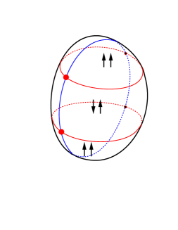
FIG. 1.: The connection between center vortices and monopoles: the (horizontal) monopole world–lines separate two patches of center vortex surface with opposite eigenvector orientations; each monopole is attached to two center vortex strings.

This close connection between monopoles and center vortices has actually been observed on the lattice [14, 15], and even presented as a puzzle [21]: on a cooled $SU(2)$ lattice configuration, almost all Abelian monopoles, identified as a $3d$ cube through which one measures a $2\pi$ magnetic flux, are attached to two opposite center vortex plaquettes. This is precisely the situation we describe: as correctly anticipated in [14, 15], Abelian monopoles and anti-monopoles are like alternating beads on a necklace formed by the center vortex string.

IV Numerical results

We have performed numerical simulations to investigate the role of the center degrees of freedom in the $SU(2)$ and $SU(3)$ lattice gauge theories. According to the discussion of the two previous sections, we have made use of the Laplacian Center Gauge fixing to reduce the symmetry to the center subgroup. In this approach – considering for instance $SU(3)$ – we have described how center vortices can be detected by looking for the points $x$ where, for example, $\phi_{1,2}^{(2)}\,{}^{\prime}(x)=0$ or, equivalently, $\phi^{(2)}(x)$ describes a $2\pi$ rotation in color space around the $\lambda_{3}^{\prime}$ axis, moving along a closed contour encircling $x$. The method is the same for a generic group $SU(N)$. As a by-product, monopole world–lines are identified by the points $x$ where two eigenvalues of $\Phi^{(1)}\,{}^{\prime}(x)$ are equal; but our aim here is to study the center degrees of freedom and not the Abelian ones. Numerical simulations are performed on a lattice and so the eigenvectors of the adjoint Laplacian operator can be computed only at discrete points. This implies that an interpolation procedure must be defined to detect center vortices and, if desired, monopoles. We have tried several interpolation methods in order to investigate the robustness of the results with respect to different choices. Unfortunately, the arbitrariness introduced by this necessary step seems large at the lattice spacings we considered. We have found only one plaquette-based interpolation scheme which guarantees that center vortex surfaces are closed. It is identical to the construction of [22], eq.(10). Remarkably, this interpolation scheme gives center vortices at locations which coincide with the $P$-vortices obtained after center projection by Greensite and collaborators [3]. Following this prescription, every gauge fixed link $U_{\mu}(x)$ is decomposed as the product of two parts

$$U_{\mu}(x)=Z_{\mu}(x)\cdot U_{\mu}^{\prime}(x)$$ (18)

where $Z_{\mu}(x)$ is the center projected link living in $Z_{N}$ and $U_{\mu}^{\prime}(x)$ is the coset link taking values in $SU(N)/Z_{N}$. For instance, this splitting can be carried out by requiring that $|\mbox{arg(Tr}(U_{\mu}^{\prime}(x)))|\leq\pi/N$. Thus, starting from an $SU(N)$ gauge fixed configuration, one builds up two projected configurations, made of the $Z_{\mu}(x)$ and the $U_{\mu}^{\prime}(x)$ links. Then, if $W(C)$ is a Wilson loop along the closed contour $C$, making use of the decomposition (18), one can write

$$W(C)=\sigma(C)\,W^{\prime}(C)=\left[\prod_{p\in\Sigma}\,\sigma(p)\right]W^{\prime}(C)$$ (19)

where $\sigma(p)$ is the plaquette built from center links $Z_{\mu}(x)$, and $W^{\prime}(C)$ and $\sigma(C)\equiv\prod_{p\in\Sigma}\,\sigma(p)$ are the Wilson loops evaluated with the coset links $U_{\mu}^{\prime}(x)$ and with the center links $Z_{\mu}(x)$ respectively. $\prod_{p\in\Sigma}$ is the product over all the plaquettes $p$ belonging to a surface $\Sigma$ supported on $C$; the value of $\sigma(C)$ does not depend on the choice of $\Sigma$ and, for simplicity, we can suppose that it is the planar surface bounded by $C$. Since we have fixed a gauge where $U_{\mu}^{\prime}$ is smooth, we expect that, to a reasonable approximation, $W(C)$ has a non-trivial value with respect to $Z_{N}$ if and only if $\sigma(C)$ does. In this approach, a non-trivial value for $\sigma(p)$ is the “signal” for a center vortex. We stress again that the vortices identified in this way coincide with interpolated gauge defects, which brings center projection on firmer theoretical ground.

We have collected 1000 $SU(2)$ configurations at three different values of the coupling constant $\beta=2.3$, $2.4$ and $2.5$ on a $16^{4}$ lattice; for $SU(3)$ we have generated 500 configurations on a $16^{4}$ lattice at $\beta=6.0$.

The following figure shows our measurement of the Creutz ratios $\chi(R)=-\ln(\langle W(R,R)\rangle\langle W(R-1,R-1)\rangle/\langle W(R,R-1)\rangle^{2})$ for $SU(2)$ at $\beta=2.4$ ($W(R,T)$ is the Wilson loop $R\times T$).

FIG. 2.: Creutz ratios at $\beta=2.4$. Empty circles refer to $SU(2)$, full circles to $Z_{2}$ and triangles to the coset $SU(2)/Z_{2}$. The continuous strip is the value of the string tension in the literature [23].

Empty circles refer to $SU(2)$, full circles to center projection after Laplacian Center Gauge fixing, and triangles to the coset part. The continuous strip is the value in the literature [23, 24] of the $SU(2)$ string tension for the chosen set of parameters. These numerical results show, on one hand, the flattening of the Creutz ratios in the $Z_{2}$ sector and, on the other hand, the vanishing of the Creutz ratios computed with the coset links. We have obtained similar behaviour for the other two values of $\beta$: $2.3$ and $2.5$. We have also carried out the same study for the $SU(3)$ lattice gauge theory. The next figure shows our results for the Creutz ratios in the $Z_{3}$ sector after Laplacian Center Gauge fixing of 500 configurations.

FIG. 3.: Creutz ratios at $\beta=6.0$ in the center sector $Z_{3}$ of $SU(3)$. The continuous strip is the value of the string tension in the literature [25].

The continuous strip is the value in the literature[25] of the $SU(3)$ string tension at the considered set of parameters. Also in this case, one clearly sees a nice flattening to a non-vanishing value of the Creutz ratios evaluated with the center projected links.

Therefore, our $SU(2)$ and $SU(3)$ results are qualitatively similar to those previously obtained in Direct Maximal Center gauge in $SU(2)$. They confirm the finding that the center-projected ensemble of gauge defects confines, with a string tension close to that of the original non-Abelian theory, whereas the coset ensemble does not. One difference however is apparent: the Creutz ratios tend to an asymptotic value much more slowly in Laplacian gauge than in DMC gauge. This is caused by the presence of many more close pairs of center vortices. Indeed, the vortex density is much higher, by a factor 3 to 5, than that measured in DMC gauge. A similar increase in the density of Abelian monopoles was observed previously in the Laplacian Abelian gauge [20]. One may consider this a practical nuisance, since these additional vortex pairs make the extraction of the projected string tension more noisy. One may instead consider that the center-projected ensemble represents the original one more closely, since it partially reproduces the short-distance increase of the force.

Finally, one can compare DMC and Laplacian Center gauges from the point of view of the computer effort. Because two eigenvectors of the adjoint Laplacian must be computed, one may get the impression that the Laplacian gauge is computationally expensive. That impression is misleading. Using the public-domain package ARPACK [26] to solve the eigenvalue problem, the computer time needed to gauge fix one $16^{4}$ configuration is about the same as for 50 Monte Carlo sweeps in the case of $SU(2)$, and 300 to 500 for $SU(3)$. This is far less than required to fix to DMC gauge iteratively.

V Interpretation of the numerical results

The figures presented in the previous section show good agreement between the Creutz ratios evaluated from the center projected ensemble of gauge defects and the value of the string tension in the literature for $SU(2)$ and $SU(3)$ at the same $\beta$. However, the importance of this numerical agreement should not be overestimated. Numerical simulations are performed at a finite value of the lattice spacing, and we see no reason to believe that, if lattice artifacts are negligible for the $SU(N)$ gauge theory, their effect is equally small on the results obtained from the center projected model. Nevertheless, our conjecture is that, even if the value of the string tension in the center sector is appreciably modified by lattice artifacts at finite lattice spacing, this dependence has to vanish in the continuum limit. The observation of such a behaviour would be a robust confirmation of the relevance of the center degrees of freedom in the confinement mechanism. In order to investigate this issue, we have considered three different lattice Laplacian operators to fix the gauge. They differ by terms which vanish in the continuum limit, i.e. higher derivatives or irrelevant operators. In practice, these new Laplacians have been obtained very simply, by smearing the links $U_{\mu}$ and substituting smeared links in the construction of the Laplacian (1). Specifically, we have considered $0$, $1$ and $5$ smearing steps (staple weight = $0.5$) on the $U_{\mu}$ links. We stress that the smeared links are used only to obtain different gauge fixing operators; the gauge transformations are always applied to the non-smeared link configurations, as well as the center projection and measurements.

The same sample of configurations has been fixed in each one of the three gauges, and the string tension has been measured in the center sector after center projection each time. In order to estimate more accurately the string tension from the $Z_{\mu}$ links, we have constructed smeared Wilson loops, where the spatial sides are made of links recursively smeared with a fixed time coordinate. This procedure is identical to that commonly used in the measurement of the $SU(N)$ static potential. It reduces the contribution of excited states, thus improving the statistical accuracy on the string tension. Although in the center projected theory, the existence of a transfer matrix is doubtful, we verified that spatial smearing did not introduce a measurable bias. From the Wilson loop data, we have extracted the $Z_{N}$ string tension using the same fitting procedure as employed for the $SU(N)$ case, with an ansatz of the form $V_{0}+\sigma R-\frac{e}{R}$ for the static potential $V(R)$

To illustrate our results, we show in the following figures the $Z_{2}$ and $Z_{3}$ Creutz ratios measured in the three gauges. The gauge dependence of the projected string tension is dramatic.

FIG. 4.: $Z_{2}$ Creutz ratios at $\beta=2.3$ in the various gauges. Full circles refer to the usual Laplacian, squares to the once-smeared and triangles to the 5-times smeared Laplacian. The continuous strip is the value of the string tension in the literature [23].

FIG. 5.: $Z_{2}$ Creutz ratios at $\beta=2.4$ in the various gauges. Full circles refer to the usual Laplacian, squares to the once-smeared and triangles to the 5-times smeared Laplacian. The continuous strip is the value of the string tension in the literature [23, 24].

FIG. 6.: $Z_{2}$ Creutz ratios at $\beta=2.5$ in the various gauges. Full circles refer to the usual Laplacian, squares to the once-smeared and triangles to the 5-times smeared Laplacian. The continuous strip is the value of the string tension in the literature [23, 24].

FIG. 7.: $Z_{3}$ Creutz ratios at $\beta=6.0$ in the various gauges. Full circles refer to the usual Laplacian, squares to the once-smeared and triangles to the 5-times smeared Laplacian. The continuous strip is the value of the string tension in the literature [25].

The string tensions $\sigma_{i}$ ($i=0,1,5$ is the number of smearing steps performed on the links $U_{\mu}$ entering in the Laplacian operator eq.(1)) obtained from our 1000 $SU(2)$ configurations at $\beta=2.3$, $2.4$, $2.5$ in the three different Laplacian Center Gauges are then compared with the $SU(2)$ string tension $\sigma_{SU(2)}$ reported in the literature. We denote by $R_{i}$ the ratio $R_{i}=\sqrt{\sigma_{i}/\sigma_{SU(2)}}$. The following table summarizes our results:

	$\qquad\beta=2.3\qquad$	$\qquad\beta=2.4\qquad$	$\qquad\beta=2.5\qquad$
$R_{0}$	$0.813(23)$	$0.860(20)$	$0.978(18)$
$R_{1}$	$0.592(12)$	$0.720(11)$	$0.804(12)$
$R_{5}$	$0.547(8)$	$0.653(7)$	$0.739(11)$

As the number of smearing steps $i$ of the links entering the Laplacian increases, the projected string tension $\sigma_{i}$ quickly decreases. This effect has nothing to do with the variation of the string tension (or absence thereof) under cooling or smearing. Here the gauge configuration is always the same unsmeared one. Only the operator used for gauge fixing changes. In this case, the reduction of the projected string tension is qualitatively easy to understand. The Laplacian made of smeared links becomes increasingly blind to short-range features of the gauge field, so that, after gauge fixing, the factorization of the Wilson loop eq.(19) into a smooth non-Abelian part $W^{\prime}(C)$ and a disordered center part $\sigma(C)$ is less effective. The smooth part $W^{\prime}(C)$ is less smooth and carries some disorder, while the center part $\sigma(C)$ is less disordered, showing a reduced string tension. However, as $\beta$ increases, the physical smearing radius $\rho$ shrinks to zero, and one expects full identification of all center vortices. Our Table shows that the numbers in each row increase with $\beta$ towards 1. The more reliable the identification of the gauge defects in the Laplacian Center Gauge, the closer the matching between the projected and the full string tensions. Thus, our numerical evidence supports the idea that a complete matching takes place in the continuum limit, i.e. center dominance (see Note Added).

If, on the other hand, the amount of smearing in our covariant Laplacian was adjusted as a function of the lattice spacing so that the physical smearing radius $\rho$ would remain constant, then one would achieve a continuum limit where, presumably, the center-projected string tension would be a fraction of the non-Abelian one. This fraction should decrease as the smearing radius $\rho$ grows. When $\rho$ reaches the physical size of a center vortex, the smeared Laplacian becomes blind to center vortices and the decomposition (19) becomes completely ineffective. This simple reasoning shows that the covariant operator used for the gauge fixing must be local for the center dominance scenario to be correct. Indeed, according to our Table, the more local the operator, the more faithful center projection appears to be at any finite lattice spacing.

A similar analysis has been carried out for $SU(3)$ and the following table shows the corresponding results:

	$\qquad\beta=6.0\qquad$
$R_{0}$	$0.93(6)$
$R_{1}$	$0.818(32)$
$R_{5}$	$0.739(24)$

The trend is similar to $SU(2)$. Furthermore, the ratios $R_{i}$ are very close to those measured in $SU(2)$ at $\beta=2.5$. Following the argument presented above, this indicates that the typical vortex size, in lattice units, is the same in both cases. With $a(SU(3),\beta=6.0)\approx 0.1$ fm and $a(SU(2),\beta=2.5)\approx 0.085$ fm, we obtain that the ratios of $SU(3)$ over $SU(2)$ center vortex sizes is about $0.1/0.085\sim 1.18$. Such a slight increase is consistent with the expected increase of the adjoint string-breaking distance [27], which is connected to the center vortex size [28].

VI Summary and discussion

The standard iterative local maximization methods used to fix the gauge on the lattice are ambiguous: they stop when any local maximum has been reached. Because of this ambiguity, one tends to mistrust measurements performed in such ill-defined gauges, as well as the physical models based on these measurements. This applies in particular to the scenario of vortex dominance, according to which the string tension of the non-Abelian theory can be exactly reproduced by considering only its center degrees of freedom, identified after gauge-fixing. Evidence for this scenario comes exclusively from lattice studies using ambiguous gauges. Some amount of counter-evidence [8, 9] has also been reported, again in similar ambiguous gauges.

Motivated by our skepticism, we have constructed, by generalizing the approach of [11], a gauge which smooths the adjoint $SU(N)/Z_{N}$ field like the usual Maximal Center Gauge (MCG), but has no ambiguity. After gauge fixing to this Laplacian Center Gauge, a remaining local $Z_{N}$ gauge freedom subsists. The local gauge defects which appear in this gauge are of two types: co-dimension 2, where the remaining gauge freedom is enlarged from $Z_{N}$ to $U(1)$, i.e. to accommodate a $U(1)$ subgroup; and co-dimension 3, where it is further enlarged to accommodate an $SU(2)$ subgroup. These two types of defects can be identified with center vortices and Abelian monopoles respectively, with the latter embedded in the former. Thus we provide a natural, unified description of these two objects which had been considered as alternative choices of effective degrees of freedom.

We have numerically implemented the Laplacian Center Gauge for $SU(2)$ and $SU(3)$. In addition to being free of the ambiguities which plague the Maximal Center Gauge, our gauge is also computationally cheaper. The gauge defects obtained by local interpolation of the Laplacian eigenvectors coincide with the $P$-vortices obtained by center projection. A measurement of Creutz ratios in the center-projected $Z_{2}$ and $Z_{3}$ ensembles superficially confirms earlier observations made in MCG, albeit with a higher density of center vortices: the center-projected ensemble confines like the original one, while the coset $SU(N)/Z_{N}$ ensemble does not. Upon closer scrutiny however, the center-projected string tension is smaller than the original one. The difference between the two can be varied by arbitrary amounts, by adding higher derivative terms to the Laplacian used for the gauge fixing. Nevertheless, we have shown evidence that this difference decreases as the continuum limit of the lattice theory is approached. The gauge dependence of the center-projected string tension, clearly visible at finite lattice spacing $a$, appears to go away as $a\rightarrow 0$. Therefore, while our study calls attention to lattice artifacts in the center projection, it gives support to the center dominance scenario.

Since the center degrees of freedom (d.o.f.) reproduce the non-Abelian confinement, one may wonder if the center-projected model can also reproduce other non-perturbative features of the non-Abelian one, like chiral symmetry breaking or topological susceptibility. Indeed, one would expect this to be the case, since the coset $SU(N)/Z_{N}$ ensemble appears deprived of all these non-perturbative features [6]. However, one encounters two difficulties when trying to measure the appropriate observables in the $Z_{N}$ model: lattice artifacts and non-positivity of the transfer matrix.

We have already emphasized how lattice artifacts, in the choice of the discretized Laplacian or in the interpolation/center projection step, can affect the matching of the $Z_{N}$ string tension with the $SU(N)$ one. Lattice artifacts modify the center vortex density so strongly that we cannot really quote a value for this important quantity. They also strongly influence the measurement of the chiral condensate in the $Z_{N}$ ensemble[5]. Naturally, they also make it conceptually difficult to define a topological charge on the lattice, especially for a discrete $Z_{N}$ theory.

Another, fundamental, difficulty comes from the non-locality of the gauge condition. After gauge fixing, all gauge links are correlated with each other, and this correlation persists after center projection. Furthermore, it may not die out exponentially at large distances in the center-projected ensemble, making it impossible to define a local effective Hamiltonian and a positive transfer matrix. Indeed, we have observed symptoms of this disease when attempting to measure glueball masses in the $Z_{N}$ ensemble: in several cases, correlations at large distances would become significantly negative, and impossible to interpret as the Euclidean-time propagator of a superposition of eigenstates of a Hamiltonian. Difficulties have also been reported for the Abelian projection [29, 30]. Symptoms may even be present for the string tension, since in Ref.[20], Creutz ratios measured after Abelian projection in the Maximal Abelian Gauge appear to increase with distance; a proper, normal decrease was restored when using instead the Laplacian Abelian Gauge. We also observed a similar increasing behaviour for the $Z_{N}$ Creutz ratios when we applied Direct Maximal Center Gauge to our $SU(2)$ configurations [31]. One may wonder if the center d.o.f. are responsible for some non-perturbative features of the Yang-Mills theory, like the string tension, and not for others, like the glueball mass. Or one may speculate that a local effective Hamiltonian can indeed be defined after center projection, but that an imperfect identification of the center d.o.f. spoils this construction: this would be one way to explain why a proper, decreasing behaviour of the Creutz ratios is restored in the Laplacian gauge. One bold attitude towards this problem is to make an ansatz for this effective Hamiltonian and test its consequences [32]. Much work remains to be done in studying the role and the interaction of the center d.o.f.

Here we have tried to put on firmer numerical ground the first step in this ambitious program, namely that $Z_{N}$ center degrees of freedom are responsible for the full string tension of the $SU(N)$ theory. In this process, we have clarified the meaning of center vortices and Abelian monopoles as local gauge defects: each monopole is pierced by a center-vortex string. Monopoles and anti-monopoles alternate along the center-vortex string like beads on a necklace. Furthermore, the eigenvectors of the covariant adjoint Laplacian, whose color orientations are used to fix the gauge, are analogous to the adjoint Higgs field in the Georgi-Glashow model. And our Abelian monopoles, which we identify via zeros of the Higgs field, are analogous to the ’t Hooft-Polyakov monopoles. Center vortices appear when a second adjoint Higgs field is considered.

Let us speculate further on a possible scenario for the complementary role of monopoles and center vortices. We consider 3 distance regimes for the force between static charges: $(i)$ At large distances $r>r_{2}$, center vortices are the relevant degrees of freedom; they govern the behaviour of the Wilson loop in all group representations, and in particular give the correct fundamental string tension and the correct, vanishing adjoint string tension. $(ii)$ At intermediate distances $r_{1}<r<r_{2}$, center d.o.f. are insufficient to describe the non-Abelian theory, and the Abelian monopoles must be considered; this generates a linearly rising potential in the adjoint and higher representations, with Abelian Casimir ratios (2 instead of 8/3 for adjoint $SU(2)$). $(iii)$ At short distances $r<r_{1}$, the full non-Abelian nature of the color field must be considered, to ensure recovery of the one-gluon exchange perturbative potential. In other words, the original non-Abelian d.o.f. can be progressively decimated, down to Abelian then center ones, as one considers larger distances.

In this scenario, the distances $r_{1}$ and $r_{2}$ separating the three regimes are related to the typical sizes of a monopole and a center vortex respectively: $(i)$ an Abelian description of the monopole field is sufficient when one stays outside its core; and $(ii)$ at large distances, the monopole field can be further approximated by that of the center vortex which pierces it. Statement $(i)$ is well-known: the regular $SU(2)$ gauge field of a ’t Hooft-Polyakov monopole can be gauge-transformed to a “stringy” gauge, where the gauge field is singular along a Dirac string (e.g. $x=y=0,z<0$), and where the flux of the Dirac string is cancelled by the Higgs field. In that gauge, the gauge field is Abelian outside the core of the monopole. To justify statement $(ii)$, one can choose a gauge where the gauge field is singular along a whole line ($x=y=0$) rather than a half-line ($x=y=0,z<0$) [33]. In that gauge also, the gauge field is Abelian outside the monopole core. Moreover, at large $|z|$ it is the same as that given by a center vortex piercing the monopole along $x=y=0$.

However, while the existence of a scale $r_{1}$ below which an Abelian description breaks down seems inevitable, that of a separate scale $r_{2}>r_{1}$ where center d.o.f. “kick in” is less so. One may say that center vortices screen the monopoles. We also find support for this scenario in theoretical studies of the Georgi-Glashow model [34, 35], which argue that the ’t Hooft-Polyakov monopoles present in this model become irrelevant at large distances, and that confinement is produced by center vortices instead. Ref.[35] in particular builds explicitly a classical solution which looks like a ’t Hooft-Polyakov monopole at short distances, and a pair of center vortices at large distances.

Note Added. Since the completion of this paper, further work [36] extending the study of [9] has appeared. The results of Refs.[9, 36] can be summarized as follows: in the iterative Maximal Center Gauge, a larger value of the gauge-fixing functional yields a smaller value of the center-projected string tension. It is then doubtful whether the latter can be equal to the non-Abelian string tension in the limit where the global maximum of the gauge-fixing functional is approached and the physical volume sent to infinity. The authors of [9, 36] and those of [10] vary in the interpretation of these numerical results, but concur that they put the usefulness of the Maximal Center Gauge in jeopardy. Our own interpretation is the following. Because of the lattice periodic boundary conditions, every gauge defect (monopole in a time-slice, center vortex in a plane) must be paired with another opposite one. Therefore, a gauge which is sufficiently non-local may bring together the locations of the members of each pair, and produce no net defect at all after projection. This may well be what happens: in the effort to approach the global maximum, defect pairs annihilate and the projected string tension drops. This illustrates that the pursuit of the global maximum is of marginal interest, whereas it is essential to pay attention to the locality of the gauge condition (in our case, of the operator used to fix the gauge), as we have emphasized in the discussion Section V. A similar claim that the Maximal Abelian Gauge suppresses monopoles excessively, but that the Laplacian gauge does not, was already argued in [20].

Acknowledgements: We thank C. Alexandrou, L. Cosmai, S. Dürr, M. D’Elia, J. Fröhlich, M. García Pérez, J. Greensite, J. Stack and T. Tomboulis for helpful discussions.

REFERENCES

- [1] G. ’t Hooft, Nucl. Phys. B 138, 1 (1978).
- [2] G. Mack and V. B. Petkova, Ann. Phys. (NY) 123, 442 (1979).
- [3] L. Del Debbio et al., Phys. Rev. D 55, 2298 (1997).
- [4] L. Del Debbio et al., Phys. Rev. D 58, 094501 (1998).
- [5] C. Alexandrou, Ph. de Forcrand and M. D’Elia, Nucl. Phys. B Proc. Suppl. 83-84, 437 (2000).
- [6] Ph. de Forcrand and M. D’Elia, Phys. Rev. Lett. 82, 4582 (1999).
- [7] A. Gonzalez-Arroyo and A. Montero, Phys. Lett. B 442, 273 (1998).
- [8] T. Kovacs and E. T. Tomboulis, Phys. Lett. B 463, 104 (1999).
- [9] V. Bornyakov et al., JETP Lett. 71, 231 (2000).
- [10] R. Bertle, M. Faber, J. Greensite, S. Olejnik, hep-lat0007043.
- [11] J. C. Vink and U. J. Wiese, Phys. Lett. B 289, 122 (1992).
- [12] J. C. Vink, Phys. Rev. D 51, 1292 (1995).
- [13] Ph. de Forcrand and M. Pepe, hep-lat/0010093; C. Alexandrou, Ph. de Forcrand and E. Follana, hep-lat/0008012.
- [14] L. Del Debbio et al., hep-lat/9708023, proceedings of “Zakopane 1997, New developments in quantum field theory”, Plenum Press, p.47.
- [15] J. Ambjorn, J. Giedt and J. Greensite, JHEP 0002 (2000) 033.
- [16] G. ’t Hooft, Nucl. Phys. B 190, 455 (1981).
- [17] S. Mandelstam, Phys. Rep. 23C, 245 (1976).
- [18] M. Faber, J. Greensite, S. Olejnik, Phys. Lett. B 474, 177 (2000).
- [19] P. van Baal, Nucl. Phys. B Proc. Suppl. 42, 843 (1995).
-
[20]
A. van der Sijs, Nucl. Phys. B Proc. Suppl. 53, 535 (1997);
A. van der Sijs, Prog.Theor.Phys.Suppl. 131 (1998) 149-159. - [21] J. D. Stack, talk at “Confinement 2000”, Osaka, March 2000; see contribution to Proceedings (World Scientific pub.).
- [22] K. Kajantie et al., hep-ph/9803367.
- [23] C. Michael and M. Teper, Phys. Lett. B 199, 95 (1987).
- [24] G. S. Bali, K. Schilling and C. Schlichter, Phys. Rev. D 51, 5165 (1995).
- [25] G. S. Bali, K. Schilling, Phys. Rev. D 47, 661 (1993).
- [26] See http://www.caam.rice.edu/software/ARPACK/.
- [27] Ph. de Forcrand and O. Philipsen, Phys. Lett. B 475, 280 (2000).
- [28] M. Faber, J. Greensite and S. Olejnik, Phys. Rev. D 57, 2603 (1998).
- [29] O. Miyamura, private communication.
- [30] J. D. Stack and R. Filipczyk, Nucl. Phys. B 546, 333 (1999).
- [31] Ph. de Forcrand and M. Pepe, hep-lat/0008013.
- [32] M. Engelhardt and H. Reinhardt, hep-lat/9912003, hep-th/0007229; M. Engelhardt, hep-lat/0004013.
- [33] J. Arafune et al., J. Math. Phys. 16 (1975) 433.
- [34] J. Ambjorn and J. Greensite, JHEP 9805 (1998) 004.
- [35] J. Cornwall, Phys. Rev. D 59, 125015 (1999).
- [36] V. G. Bornyakov, D. Komarov and M. Polikarpov, hep-lat/0009035.