Meson correlators in finite temperature lattice QCD

Abstract

We analyze temporal and spatial meson correlators in quenched lattice QCD at $T\geq 0$. Below $T_{c}$ we observe little change in the meson properties as compared with $T=0$. Above $T_{c}$ we observe new features: chiral symmetry restoration and signals of plasma formation, but also indication of persisting “mesonic” (metastable) states and different temporal and spatial “masses” in the mesonic channels. This suggests a complex picture of QGP in the region $1\,-\,1.5\,T_{c}$.

1 Introduction

With increasing temperature, hadronic correlators are expected to change their nature drastically (see, e.g., [1], [2]). At the critical temperature, the deconfinement of color degrees of freedom and the restoration of the chiral symmetry are expected to occur simultaneously. Two “extreme” pictures are frequently used to describe the low and the high $T$ regimes, respectively: the weakly interacting meson gas, where we expect the mesons to become effective resonance modes with a small mass shift and width due to the interaction; and the perturbative quark gluon plasma (QGP), where the mesons should eventually disappear and (at very high $T$) perturbative effects should dominate.

Near to the critical temperature, however, the actual physical situation is more involved. The interaction with a hot meson gas and with baryonic matter have been studied in various phenomenological models which predict appreciable changes in the vector meson properties (see, e. g., [3]). In a NJL model [4] the scalar and the pseudo-scalar modes are found to correlate strongly, and to subsist even above the transition as so-called “soft modes”, corresponding to narrow peaks in the spectral function and realized as the fluctuation of the order parameter of the chiral symmetry restoration transition. On the other hand, at the short distance scale, the fundamental excitation should be quarks and gluons. Lattice QCD results on the quark number susceptibility support this view [5]. These pictures may not be contradicting each other: DeTar conjectured the existence of excitations in the QGP phase corresponding to different distance scales, and pointed out to the possibility of “confinement” still ruling the large distance scales [6]. While with increasing temperature the physics should appear increasingly dominated by quark and gluon degrees of freedom, in accordance to the perturbative high temperature picture, the intermediate temperature range above $T_{c}$ seems to be much more complex and dominated by strongly interacting quarks (see also [7]), which, as we shall see below, even tend to stay strongly spatially correlated and thus agree with a picture of effective, low energy modes in the mesonic channels. Since these matters are related to questions about the evolution of the early universe, on one hand, and to the interesting results from heavy ion collision experiments [8], where QGP conditions are being realized [9], on the other hand, it is important to have quantitative estimates in addition to qualitative understanding and we need model-independent studies of the hadronic correlators at finite temperature.

Lattice simulations are the most powerful instrument at present to investigate such problems in the fundamental theoretical framework of quantum chromodynamics (QCD). Extensive studies have been dedicated to the thermodynamics of the finite temperature transition (see, e. g., [10],[11]). Concerning the hadronic sectors, numerical analysis of “screening” (spatial) propagators indicate correlated (bound?) quarks while the mesonic “screening masses” increase toward the 2-free quark threshold ($2\pi T$, induced by the anti-periodic boundary conditions in the temporal direction) [12]. Since the spatial directions can (and must) be made large, these propagators are unproblematic in principle and can be studied as well as for $T=0$: at any $T>0$ the propagation in the space directions represents in fact a $T=0$ problem (with asymmetric finite size effects). The interpretation of the results from “screening” correlators in terms of modes of the temporal dynamics is far from straightforward, however: since in the Euclidean formulation the $O(4)$ symmetry is broken at $T>0$ (see, e.g., [14]), physics appears different depending on whether we probe the space (“$\sigma$”: $\vec{x}$) or time (“$\tau$”: $t$) direction. The static quark potential associated to propagation in a spatial direction, for example, is a very anisotropic quantity which above $T_{c}$ still grows linearly in two of the spatial directions (confines), in contrast to the potential associated to the propagation in the $t-$direction which is isotropic and not confining. Therefore we need to investigate hadronic correlators with full “space-time” structure, in particular the propagation in the Euclidean time.

Ideally, what we should like to do is to reconstruct the spectral function in the given channel. Then we could directly compare with the results from heavy-ions experiments, see e. g., [8]. The spectral function at finite temperature can be extracted from the correlators in the (Euclidean) temporal direction whose extent $l_{\tau}$ is related to the temperature as $T=1/l_{\tau}$ [14, 15]. These data (after Fourier transforming the $t$-correlators) are given at discrete Matsubara frequencies on the imaginary energy axis and are affected by errors. The extraction of the spectral function implies (logically) an interpolation and an analytic continuation to the real energy axis. For a numerical analysis, which produces a finite amount of information, this is an improperly posed problem. Its solution is dependent on imposing supplementary conditions (“a priori information”) to regularize the algorithms and to prevent the amplification of the errors. These conditions can be either based on general, statistical arguments (e.g. variance limitation, Bayesian analysis, maximal entropy method) or on particular, physical expectations (e.g., using an ansatz for the spectral function which leads to an explicit analytic form for the correlator, to be fitted against the data). We should, however, be aware of the fact that all regularization introduces a bias and therefore this problem is fundamentally intricate.

The main difficulty in the numerical calculation at $T>0$ originates in the short temporal extent $l_{\tau}=1/T$. Beyond the general necessity of producing enough and precise data the $T>0$ problem is doubly complicated as compared to the $T=0$ one: on one hand the structure we may expect is more complex than just a pole, on the other hand the time extent of the propagation cannot be made large to select the low energy contributions. We shall now briefly discuss this questions and thereby also introduce our procedure to deal with them.

1) Lattice problems: Large $T$ can be achieved using small $N_{\tau}=l_{\tau}/a$ ($a$: lattice spacing), however this leads to systematic errors [16]. Moreover, having the $t$-propagators at only a few ($N_{\tau}/2$) points makes it difficult to characterize the unknown structure in the corresponding channels: practically any ansatz can be fitted through 2-3 points! To obtain a fine $t$-discretization and thus detailed $t$-correlators, while avoiding prohibitively large lattices (we need large spatial size in order to avoid finite size effects, typically $l_{\sigma}\sim 3l_{\tau}$), we proposed [17, 18] to use different lattice spacings in space and in time, $a_{\sigma}/a_{\tau}=\xi>1$ [19]. The renormalization analysis of such lattices, however, is more involved, because of the supplementary parameter $\xi$ and this introduces also some uncertainties.

2) Physical problems: The low energy structure of the mesonic channels cannot be observed directly, due to the inherently coarse resolution $2\pi T=2\pi/l_{\tau}$ of the imaginary energy axis. Refining the discretization of the time axis improves the fitting and analytic continuation problem, but although we are following the question of the spectral analysis we do not have yet reliable results at $T>0$ for this challenging question. Our problem setting here is therefore more limited: we shall try to recognize mesonic states and ask about their character and properties at various temperatures.

In this paper, we investigate the full four-dimensional structure of the meson correlators on an anisotropic lattice in the quenched approximation. Thus the phase transition is the deconfining one, and the hadronic correlators are constructed with quark propagators on the background gauge field.

Our strategy here is the following: we first select the mesonic ground states of the $T=0$ problem (where the time direction can be made sufficiently large – about 3.2 fm in our case, which, at the quark masses we work with, means about 8 pion correlation lengths) and characterize their internal structure by measuring the (Coulomb gauge) wave functions. Then we ask whether states characterized by similar internal structure can be retrieved at higher temperature, try to reconstruct them with help of correspondingly smeared sources and investigate how they are affected by the temperature. If the changes in the correlators are small, which is consistent with mesons interacting weakly with other hadron-like modes in the thermal bath, this procedure allows us to define “effective modes”. Large changes will signal the breakdown of this weakly interacting gas picture and there we must try to compare our observations with other pictures, in particular the perturbative QGP.

The meson correlators in the temporal direction play a central role in this study, which is therefore meant to supplement other approaches, including studies of screening propagators [12], [13]. To understand the effect of fixing a mesonic source we employ three kind of meson operator smearing. The propagators and the wave functions are also compared with those of mesons composed of free quark propagators (“free” mesons) . Finally we attempt a chiral limit; note, however, that even with anisotropic lattices the short physical extent in the temporal direction makes the quantitative estimate of the (temporal) masses (if they exist) difficult. Our program should not be understood as an alternative for a study of the spectral function at $T>0$, but as an attempt to answer some special questions about the phenomena in QGP. In that sense our results only offer partial views.

To prevent a certain confusion we stress here that we do not look for the eigenstates of the Hamiltonian (transfer matrix), which show up as asymptotic states for $t\rightarrow\infty$ at $T=0$. At non-zero temperature the physical processes are essentially dependent on the mixtures induced by the thermal bath. For the physical picture and for building models the question is whether these phenomena can be described in terms of some effective excitations (quasi-particles [20]), which “replace” thus the fundamental particle modes, or completely new states dominate the physics above some $T$.

Our analysis proceeds in three steps:

• Analysis of temporal propagators. Here we try to see what kind of excitations propagate in the mesonic channels at $T>0$ based on the $t-$dependence of these propagators (“effective mass” $m(t)$).

• Analysis of the “Coulomb gauge wave functions”. Here we study the behavior of the temporal correlators with the distance between $q$ and ${\bar{q}}$ at the sink, which provides us with information of the spatial correlation between the quarks at given $t$.

• Analysis of the temperature dependence of the temporal and spatial masses of the putative states which are compatible with the behavior observed at the previous steps.

Note that due to the quenched approximation the dynamics is incomplete. In a strong sense the Hamiltonian does not posses true mesonic states and only provides the gluonic interactions responsible for the forces binding the quarks. This is not a problem specific to nonzero temperature but is the same already at $T=0$. The success of the spectrum calculations at $T=0$ indicates, however, that one should not consider quenched QCD as a theory by itself but as an approximation to the full theory (which posses genuine asymptotic mesonic states) and the exclusion of $q$-$\bar{q}$ pair creation as a reasonably small error at least concerning some of the characteristics of the hadrons. In particular, we observe strong indication of chiral symmetry restoration above the transition temperature.

The paper is organized as follows. In the next section we describe our analysis strategy in some more detail. Section 3 describes the preparation of the lattice: the introduction of anisotropic lattice actions and the simulation parameters (the “calibration”, i.e. the tuning of the anisotropy parameters, is described in detail in the Appendix). The subsequent two sections present the results of the simulation: In Section 4 we observe the correlators at zero temperature and discuss the source smearing and the variational analysis. The results at finite temperature are presented in Section 5. The last section is reserved for discussion and outlook.

2 Analysis strategy

2.1 Comments on the physical problems

We here should like to illustrate the problems raised by the finite temperature and the question of the source in the frame of our approach. The reader who is familiar with these problems may skip this section.

Let us consider that we use some meson operator $\Phi$, then the propagator at $\beta\equiv 1/T<\infty$ in Euclidean time $t>0$ is:

$$G^{(\Phi\rightarrow\Phi)}_{\beta}(t) = \langle\Phi(t)\Phi(0)\rangle=\frac{1}{Z}\int_{(a)pbc}\Phi(t)\Phi(0){\rm e}^{-\int_{0}^{\beta}{\cal L}}$$ (1)

$$= \frac{1}{Z}{\rm Tr}\left[{\cal T}^{N_{\tau}-t}\Phi{\cal T}^{t}\Phi\right]={\rm Tr}\left[{\rm e}^{-\beta\,H}{\rm e}^{t\,H}\Phi{\rm e}^{-t\,H}\Phi\right]/{\rm Tr}\left[{\rm e}^{-\beta\,H}\right]$$ (2)

$$= \sum_{n,k}{\rm e}^{-(\beta-t)\,E_{n}-t\,E_{k}}\langle\phi_{n}|\Phi|\phi_{k}\rangle\langle\phi_{k}|\Phi|\phi_{n}\rangle/\sum_{n}{\rm e}^{-\beta\,E_{n}}$$ (3)

$$= \sum_{n,k}{\rm e}^{-\frac{\beta}{2}(E_{n}+E_{k})}c_{nk}^{2}{\rm cosh}\left[(\beta/2-t)(E_{k}-E_{n})\right]/\sum_{n}{\rm e}^{-\beta\,E_{n}}$$ (4)

where ${\phi_{n}}$ are eigenstates of the Hamiltonian representing, say, (multi-)meson states and other hadron-like modes and we have:

$$\langle\phi_{n}|\Phi|\phi_{k}\rangle=c_{nk},\ \ c_{kn}=c^{*}_{nk}=c_{nk}$$ (5)

Here we expressed everything in units of $a_{\tau}(a_{\tau}^{-1})$, hence $\beta=N_{\tau}$; ${\cal T}={\rm exp}(-H)$ is the transfer matrix. For $T=0$ only the vacuum $n=0$ survives in the sum over $n$ in (3). Assume each $\Phi$ selects not only the mesonic ground state, say $|\phi_{1}\rangle$, but also some other, excited states, then

$$\langle\phi_{k}|\Phi|\phi_{0}\rangle\simeq c_{01}\delta_{k,1}+c_{02}\delta_{k,2}+\dots$$ (6)

and the zero temperature propagator is (we put $E_{0}=0$ for simplicity):

$$G^{(\Phi\rightarrow\Phi)}_{\infty}(t)\simeq c_{01}^{2}{\rm e}^{-t\,E_{1}}+c_{02}^{2}{\rm e}^{-t\,E_{2}}+\dots$$ (7)

Hence the lightest state contribution will dominate at large $t$. Tuning a “perfect” source at $T=0$ we ideally achieve $c_{0k}=0$ for $k\neq 1$ and thus see only this contribution at all $t$. Suppose that we have been able to construct in this way a “perfect” operator $\Phi_{1}\sim a+a^{{\dagger}}$, with $a(a^{{\dagger}})$ the annihilation (creation) operator for a meson in the ground state. Then at $T=0$ $G$ reduces to the first term, as desired

$$G^{(\Phi_{1}\rightarrow\Phi_{1})}_{\infty}(t)\simeq c_{01}^{2}{\rm e}^{-t\,E_{1}}$$ (8)

(note that correlators with different operators at the source and the sink also project only on the ground state if either the source or the sink is “perfect”). With increasing $T$, however, further states beyond the vacuum survive in the sum over $n$ and acting on each of them $\Phi_{1}$ “adds/subtracts” a meson to whatever is there, correspondingly selecting from the inner sum the states $k$ onto which this new state projects, $\langle\phi_{n}|\Phi_{1}|\phi_{k}\rangle\neq 0$, in a sloppy notation $k\in\{n_{\pm 1}\}$. Instead of (8) the correlator is now a sum of contributions and we ask whether this mixture can be described by an effective mode $|{\tilde{\phi}}_{1}\rangle$ of energy ${\tilde{E}}_{1}^{({\beta})}$ such that we can write, similarly to the $T=0$ expression:

$$G^{(\Phi_{1}\rightarrow\Phi_{1})}_{\beta}(t) = \sum_{n}\sum_{k\in\{n_{\pm 1}\}}{\rm e}^{-\frac{\beta}{2}(E_{n}+E_{k})}c_{nk}^{2}\cosh\left[\left(\frac{\beta}{2}-t\right)(E_{k}-E_{n})\right]/\sum_{n}{\rm e}^{-\beta\,E_{n}}$$ (9)

$$\sim {\rm cosh}\left[\left({{\beta}\over 2}-t\right){\tilde{E}}_{1}^{({\beta})}\right].$$

To fix the ideas let us consider an oscillator with frequency $\omega$ and a small anharmonic perturbation:

$$H=H_{0}+\epsilon H_{\rm I}$$ (10)

(this may be considered a caricature of a weakly interacting meson gas, say). To first order in $\epsilon$ we can use the unperturbed basis to calculate the propagator $G(t)$. Let $\Phi_{1}$ be the ground state operator,

$$\Phi_{1}=(a+a^{{\dagger}})/\sqrt{2\omega}\ ,\ \ \langle\phi_{k}|\Phi_{1}^{{\dagger}}|\phi_{n}\rangle=\frac{1}{\sqrt{2\omega}}\left(\sqrt{n+1}\delta_{k,n+1}+\sqrt{n}\delta_{k,n-1}\right)\ ,$$ (11)

then we have:

$$G^{(\Phi_{1}\rightarrow\Phi_{1})}_{\beta}(t)=\frac{1}{\omega}\sum_{n\geq 1}n{\rm e}^{-\beta\,(E_{n}-\frac{1}{2}\Delta_{n})}{\rm cosh}\left[\left(\frac{\beta}{2}-t\right)\Delta_{n}\right]/\sum_{n\geq 0}{\rm e}^{-\beta\,E_{n}}$$ (12)

For the unperturbed oscillator ($\epsilon=0$):

$$E_{n}=\left(n+\frac{1}{2}\right)\omega,\ \ \Delta_{n}\equiv E_{n}-E_{n-1}=\omega.$$ (13)

Then the $t-$dependence factorizes in (12) and we have a trivial effect of the temperature:

$$G^{(\Phi_{1}\rightarrow\Phi_{1})}_{osc.,\,\beta}(t)=\frac{{\rm cosh}\left[\left(\frac{\beta}{2}-t\right)\,\omega\right]}{2\,\omega\,{\rm sinh}\left[\frac{\beta}{2}\,\omega\right]}{\!\begin{array}[]{c}\vspace*{-0.2cm}{}\hfil\\ {\longrightarrow\vspace*{-0.2cm}}\\ {\scriptscriptstyle{\beta\rightarrow\infty}}\end{array}\!}{\rm e}^{-\omega\,t}.$$ (14)

If we turn on the interaction the levels are no longer equidistant (the effect of adding one more meson depends on the total number of mesons present in the state) and the $t-$dependence is non-trivially affected by temperature. We write:

$$\Delta_{1}={\tilde{\omega}},\ \ \Delta_{n\geq 2}={\tilde{\omega}}-\epsilon\,\lambda_{n},$$ (15)

then to first order in $\epsilon$ (weakly interacting gas)

$$G^{(\Phi_{1}\rightarrow\Phi_{1})}_{w.i.g.,\,\beta}(t)\propto{\rm cosh}\left[\left(\frac{\beta}{2}-t\right)\,{\tilde{\omega}}^{({\beta})}\right]+{\cal O}(\epsilon^{2})$$ (16)

with

$${\tilde{\omega}}^{({\beta})}={\tilde{\omega}}-\epsilon\,\frac{\sum_{n\geq 1}\lambda_{n+1}\,(n+1)\,\,{\rm e}^{-\beta\,E_{n}}}{\sum_{n\geq 0}(n+1)\,{\rm e}^{-\beta\,E_{n}}}{\!\begin{array}[]{c}\vspace*{-0.2cm}{}\hfil\\ {\longrightarrow\vspace*{-0.2cm}}\\ {\scriptscriptstyle{\beta\rightarrow\infty}\ {\rm or}\ \epsilon\rightarrow 0}\end{array}\!}{\tilde{\omega}}{\!\begin{array}[]{c}\vspace*{-0.2cm}{}\hfil\\ {=\vspace*{-0.2cm}}\\ {\scriptscriptstyle\epsilon=0}\end{array}\!}\omega.$$ (17)

Notice that the above effects show up although we use the “perfect” source $\Phi_{1}$: they represent the genuine temperature effects for an interacting system. From (16),(17) we see that as long as the interaction between the modes (“the mesons”) is weak we expect small changes which may be simulated by a shift (and possibly a widening) of the peak in the spectral function, defining in this way an effective mode (9). Large changes, on the other hand, will signal the installation of a new regime. Then we must try to obtain additional information by other tests. Essentially, this is our program. Of course in real life we shall not be able to obtain a “perfect” source in the above sense. The various uncertainties inherent in our procedure will be repeatedly discussed in the course of the paper.

If we use a “perfect” source but a different sink (with non-zero projection on the source) we reach similar expressions. To the next order in $\epsilon$, however, at $T>0$ the temperature correction to the mass will depend on the sink operator. Generally therefore at $T>0$ we expect to find sink dependence of propagators even for “perfect” source. This dependence can be seen as an indication for the importance of temperature effects.

2.2 Mesonic correlators

A first attempt to optimize the mesonic operators, in the spirit described in the previous section, is to introduce a smearing function $\omega(\vec{y})$, such that the zero-momentum mesonic operator reads:

$$\Phi_{\rm M}^{(\omega)}(t)=\sum_{\vec{z}}\sum_{\vec{y}}\omega(\vec{y})\,\bar{q}(\vec{z},t){\gamma}_{\rm M}q(\vec{z}+\vec{y},t).$$ (18)

giving rise to smeared correlators (we shall omit the index “$\beta$” in the following):

$$G_{\rm M}^{(\omega\rightarrow\omega^{\prime})}(t) = \langle{\rm Tr}\left[\Phi_{\rm M}^{(\omega^{\prime})}(t)\Phi_{\rm M}^{(\omega)}(0)\right]\rangle$$

$$= \mbox{$\sum_{\vec{z_{1}},\vec{z_{2}},\vec{y_{1}},\vec{y_{2}}}$}\,\omega^{\prime}(\vec{y_{1}})\omega(\vec{y_{2}})\,\langle{\rm Tr}\left[S(\vec{z_{2}},0;\vec{z_{1}},t)\gamma_{\rm M}\gamma_{5}S^{{\dagger}}(\vec{z_{2}}+\vec{y_{2}},0;\vec{z_{1}}+\vec{y_{1}},t)\gamma_{5}\gamma_{\rm M}^{{\dagger}}\right]\rangle$$

Here $\langle.\rangle$ means summation over Yang-Mills configurations. $S$ is the quark propagator and $\gamma_{\rm M}=\{\gamma_{5},\gamma_{1},1,\gamma_{1}\gamma_{5}\}$ for M=$\{{\rm Ps,V,S,A}\}$ (pseudo-scalar, vector, scalar and axial-vector, respectively). In the scalar sector, only the connected part of the correlator is evaluated. The Coulomb gauge is used to produce the quark propagators $S$ – this is of course irrelevant for the $\vec{y_{1}}=\vec{y_{2}}=0$ expectation values. Note that generally we keep different smearing functions at the source and the sink. This will allow, given a certain basis of operators $\{\Phi^{a}\}$, to perform a variational analysis in order to attempt a further optimization of the mesonic operator - for details see section 4.

As smearing functions we shall use two different kinds,

• A “point” source (sink):

  $$\omega_{\vec{x}}(\vec{y})\propto\delta(\vec{x}-\vec{y}).$$ (20)

  This will be mainly used to study the $\vec{x}$ dependence of the correlator

  $$G_{\rm M}^{(\omega)}(\vec{x},t)\equiv G_{\rm M}^{(\omega\rightarrow\omega_{\vec{x}})}(t)=\sum_{\vec{z}}\langle\bar{q}(\vec{z}+\vec{x},t){\gamma}_{\rm M}q(\vec{z},t)\,\Phi_{\rm M}^{(\omega)}(0)\rangle.$$ (21)

  at fixed $t$. $G_{\rm M}^{(\omega)}(\vec{x},t)$ can be interpreted as “Coulomb gauge wave-function”, it indicates the spatial correlation between quark and anti-quark.

• The convolution:

  $$\omega_{ab}(\vec{y}) = \mbox{$\sum_{\vec{v}}$}\,\omega_{a}(\vec{v})\,\omega_{b}(\vec{v}+\vec{y})$$ (22)

  which is equivalent to using smeared quark and antiquark fields with smearing functions $\omega_{b}$ and $\omega_{a}$ respectively. We use here three kinds of quark smearing functions:

  $$\omega_{p}(\vec{y}) \propto \delta(\vec{y})\ \ {\rm(}``point"{\rm)}$$ (23)

  $$\omega_{e}(\vec{y}) \propto {\rm exp}(-\,a\,|\vec{y}|^{p})\ \ {\rm(}``exp."{\rm)}$$ (24)

  $$\omega_{w}(\vec{y}) \propto 1\ \ {\rm(}``wall"{\rm)}$$ (25)

  In tuning the exponential source $exp$ in (24) we shall use the parameters $a,p$ from the observed dependence on ${\vec{x}}$ at large $t$ of the temporal Ps wave function with point-point source at $T\simeq 0$, $G_{\rm M}^{(pp)}(\vec{x},t)$ - see 21. The mesonic operator “exponentially” smeared both at the quark and the antiquark corresponds to a mesonic source in the relative $q$-$\bar{q}$ distance given by the convolution (22). Therefore the $exp$-$exp$ smearing with $a,p$ from the wave function implies a meson source typically wider than the measured wave function $G_{\rm M}^{(pp)}(\vec{x},t)$, $t\gg 1$.

The $t$ dependence of the temporal propagators $G_{\rm M}^{(\omega\rightarrow\omega^{\prime})}(t)$ depends on the spectral functions. On a periodic lattice the contribution of a pole in the mesonic spectral function to the $t$-propagator is $\propto{\rm cosh}[M(t-N_{\tau}/2)]$ (this $M$ is therefore called “pole-mass”). A broad structure or the admixture of excited states leads to a superposition of such terms. Fitting a given $t$-propagator by cosh$(m(t)(t-N_{\tau}/2))$ at pairs of points $t,t+1$

$$\frac{G(t)}{G(t+1)}=\frac{\mbox{cosh}\left[m^{(\tau)}_{eff}(t)\,(N_{\tau}/2-t)\right]}{\mbox{cosh}\left[m^{(\tau)}_{eff}(t)\,(N_{\tau}/2-t-1)\right]}$$ (28)

defines an “effective mass” $m_{eff}(t)$, which is a constant if the spectral function has only one, narrow peak. The effective mass is a rather sensitive observable which shows effects of the source dependence, widening of the spectral function or existence of excited states, without, however, allowing to differentiate among them. To the extent that the effective mass reaches a plateau and permits to define a “temporal mass” $m^{(\tau)}$ at $T>0$, the latter connects directly to the (pole) mass of the mesons below $T_{c}$, while above $T_{c}$ it will presumably help analyze the dominant low energy structure in the frame of our strategy. By contrast, using spatial propagators we shall extract the “screening mass” $m^{(\sigma)}$.

Errors are estimated by the single elimination Jackknife method, unless otherwise notified. For details see section 4. For various comparisons we shall also use in (2.2), instead of the quark propagators $S$ measured in each MC configurations, free quark propagators, defining in this way “free” mesons.

3 Lattice setup

In this section we describe the preparation of the lattice on which mesonic correlators at zero and finite temperature are calculated.

3.1 Anisotropic lattice

We use anisotropic lattices on which the spatial and the temporal lattice spacings are different: $a_{\sigma}\neq a_{\tau}$ [19]. The simplest generalization of commonly used Wilson actions for gauge and quark fields is obtained as follows.

For the gauge field action,

$$S_{G}=\frac{\beta}{\gamma_{G}}\sum_{x,i<j\leq 3}\left(1-\frac{1}{3}\hbox{ReTr}\,U_{ij}(x)\right)+\beta\,\gamma_{G}\sum_{x,i\leq 3}\left(1-\frac{1}{3}\hbox{ReTr}\,U_{i4}(x)\right)$$ (29)

where

$$U_{\mu\nu}(x)=U_{\mu}(x)U_{\nu}(x+\hat{\mu})U_{\mu}^{{\dagger}}(x+\hat{\nu})U_{\nu}^{{\dagger}}(x)$$ (30)

The bare anisotropy parameter $\gamma_{G}$ controls the ratio of spatial and temporal lattice spacings. For the fermion,

$$S_{F}=\frac{1}{2\kappa_{\sigma}}\sum_{x,y}\,\bar{q}(x)\,K(x,y)\,q(y),$$ (31)

$$K(x,y)=\delta_{x,y} - \kappa_{\sigma}\sum_{i=1}^{3}\left[(1-\gamma_{i})\,U_{i}(x)\,\delta_{x+\hat{i},y}+(1+\gamma_{i})\,U_{i}(x-\hat{i})\,\delta_{x-\hat{i},y}\right]$$ (32)

$$- \kappa_{\sigma}\,\gamma_{F}\left[(1-\gamma_{4})\,U_{4}(x)\,\delta_{x+\hat{4},y}+(1+\gamma_{4})\,U_{4}(x-\hat{4})\,\delta_{x-\hat{4},y}\right],$$

where $\kappa_{\sigma}$ is the spatial hopping parameter and $\gamma_{F}$ is the bare anisotropy for fermions. For later convenience, we define $\kappa$ as

$$\frac{1}{\kappa}\equiv\frac{1}{\kappa}-2\,(\gamma_{F}-1)=2\,(m_{0}+4),$$ (33)

where $m_{0}$ is the bare quark mass parameter in units of the spatial lattice spacing. At a later stage, we shall carry out the chiral extrapolation in this $1/\kappa$.

The actual anisotropy $\xi$ is defined using certain correlators, $F$, containing gauge and fermion fields. In general, $\gamma_{G}$ and $\gamma_{F}$ are different from $\xi$ because of the interaction [19, 21]. To obtain the desired value of $\xi$, one needs to tune the values of $\gamma_{G}$ and $\gamma_{F}$ by requiring the isotropy of correlators in physical units:

$$F_{\sigma}(z)=F_{\tau}(t=\xi\,z),$$ (34)

where t and z are understood in the corresponding lattice units, $a_{\tau}$ and $a_{\sigma}$ respectively. This renormalization procedure is called “calibration”. Since we compare the temporal and the screening masses, it is important to obtain $\xi$ as precisely as possible, and verify that these two kinds of mass coincide at $T=0$.

In the case of dynamical quarks, a precise calibration requires a large effort, since we generally have four bare parameters ($\beta$, $\gamma_{G}$, $\kappa_{\sigma}$ and $\gamma_{F}$) and only three physical parameters $\xi$, $a_{\sigma}$ and $m_{q}$ which can be varied, therefore the condition of physical isotropy implies a non-trivial constraint among the bare parameters [18]. In a quenched simulation, however, the situation is much simpler. Here one generates gauge field configurations using certain values of $\beta$ and $\gamma_{G}$ and reads $\xi$ from gluonic quantities. Then the fermionic parameters are determined such that they give the desired quark (or hadron) mass and the same $\xi$ is obtained from hadronic correlators.

3.2 Lattice parameters

We use lattices of sizes $12^{3}\times N_{\tau}$, where $N_{\tau}=72$ ($T=0$), 20 (below $T_{c}$), 16 and 12 (above $T_{c}$), with couplings $\beta=5.68$, $\gamma_{G}=4.0$, in the quenched approximation. Configurations are generated with the pseudo-heat bath algorithm with 20000 thermalization sweeps, the configurations being separated by 2000 sweeps. In most cases, 60 configurations are used, except for the calibration. The gauge field is fixed to the Coulomb gauge. The calibration is described in detail in the Appendix. From the calibration of the gauge configurations we obtain a renormalized anisotropy $\xi=5.3(1)$. The lattice cutoffs determined from the heavy quark potential are $a_{\sigma}^{-1}=0.85(3)$ GeV ($a_{\sigma}\sim 0.24$ fm) and $a_{\tau}^{-1}=4.5(2)$ GeV ($a_{\tau}\sim 0.045$ fm).

Table 1 summarizes the quark parameters and gives the meson masses as determined in the next section. As a guide for the mass range we are concerned with, the quark mass is estimated by a naive relation $m_{q}=(\kappa^{-1}-\kappa_{c}^{-1})/2$ using the critical hopping parameter $\kappa_{c}=0.17144(11)$. This simulation deals therefore with quarks in the strange quark mass region. The boundary conditions for quark fields are set to periodic and anti-periodic in spatial and temporal directions respectively, except for the calibration (at $T=0$) where anti-periodic b.c. in all four directions are used.

In the following we always display dimensionless quantities, that is, they are understood as given in the corresponding lattice spacings or their inverses. Since we have two lattice spacings, $a_{\sigma}$ and $a_{\tau}$, when we shall compare different quantities we shall use the translation $a_{\sigma}=\xi a_{\tau}$, i.e., the numbers featured can be understood as given in units of $a_{\tau}$ ($a_{\tau}^{-1}$).

$\kappa_{\sigma}$	$\gamma_{F}$	$N_{conf}$	$\kappa$	$m_{q}$	$m_{Ps}$	$m_{V}$
0.081	4.05(2)	20	0.1601	0.0389	0.1777( 8)	0.1962(10)
0.084	3.89(2)	20	0.1633	0.0276	0.1493( 9)	0.1747(12)
0.086	3.78(2)	30	0.1648	0.0223	0.1341(10)	0.1644(13)

Table 1: Quark parameters. $\gamma_{F}$ is determined by the calibration using first $N_{conf}$ configurations. The error of $\kappa$ and $m_{q}$ is not estimated ($\gamma_{F}$ is fixed in successive calculation). The tabulated meson masses are the values obtained with smeared correlators described in the next section. All masses are given in units of $a_{\tau}^{-1}$.

3.3 Finite temperature

In [23] we have measured the Polyakov loop susceptibility as a function of $\gamma_{G}$ for several values of $N_{\tau}$. At $N_{\tau}=18$, the peak was found between $\gamma=3.9$ and 4.0, which means on our $\gamma=4$ lattice that $N_{t}=18$ is very close to and just above $T_{c}$. The estimated temperature for our values of $N_{\tau}$ are therefore $T\simeq 0$, $0.93\,T_{c}$, $1.15\,T_{c}$ and $1.5\,T_{c}$ for $N_{\tau}=72$, $20$, $16$ and $12$ respectively.

We found that the configurations above $T_{c}$ stay in a single Polyakov loop sector during the whole updating history, and that the behavior of meson correlators strongly depends on the sector. The hadronic correlators feel the deconfining transition if they are taken in the real sector, but they appear not to “notice” it if they are taken on configurations in one of the complex sectors [22]. With dynamical quarks, the $Z_{3}$ center symmetry is explicitly broken and the Polyakov loop prefers to stay on the real axis. Since we regard the quenched lattice as an approximation to the dynamical lattice, we restrict our simulation to the case with real Polyakov loop sector.

4 Zero temperature analysis.

In the context of our strategy the analysis of the zero temperature correlators serves as foundation for the analysis at $T>0$. This is also a good opportunity to describe in detail our procedure. Here we obtain the meson masses and the wave function which is used to smear the source and sink operators.

Smearing of mesonic operators

To fix the exponential smearing function we measure the wave function at zero temperature, given by (21) with point smearing $\omega_{p}(\vec{y})=\delta(\vec{y})$ both for the quark and anti-quark at the source: and define

$$\omega_{e}(\vec{y})=G_{\rm M}^{(pp)}(\vec{y},t)/G_{\rm M}^{(pp)}(\vec{0},t)\large|_{t\gg 1}=\exp(-\,a\,y^{p}),$$ (35)

where $a$, $p$ are fitting parameters. The fitted values of $a$ and $p$ of the Ps meson wave function are listed in Table 2.

To extract the effective mass from the correlators following eq. (28) we have several possibilities depending on the choice of mesonic operators $\Phi_{M}^{(\omega)}(t)$. We call $m_{\rm eff}^{(\omega\rightarrow\omega^{\prime})}(t)$ the effective mass extracted from correlators smeared with $\omega$ and $\omega^{\prime}$ at the source and the sink respectively. In figure 1 we display the effective masses for $\kappa_{\sigma}=0.086$. In all cases, the sink $\omega^{\prime}$ is a $point$-$point$ operator and we show three choices of $\omega$ at the source: $point$-$point$, $point$-$exp$ and $exp$-$exp$ ($pp$, $pe$ and $ee$ respectively in what follows). For S and A channels, only the correlators with $exp$-$exp$ source are shown, since with other sources statistical fluctuations are so large that no clear plateaus are found. It is clear from the figure that the effective masses from different operators converge to the same value at large $t$, the worst behavior being observed for the non-smeared $pp$-$pp$ correlator. Considerable improvement is observed for the masses extracted from smeared operators. Of them $m_{\rm eff}^{(ee\rightarrow pp)}(t)$ is the one that converges most rapidly to a plateau, though it increases slightly at early stages, which is due to the fact that the source is slightly too wide, as discussed in section 2.2. The amount of optimization achieved by the exponentially smeared operator has to be analyzed through the diagonal correlator $\langle\Phi_{M}^{ee}(t)\Phi_{M}^{ee}(0)\rangle$ which is a sum of positive contributions from the different states – see (7), (8). In Fig. 2 we show, in addition to the off-diagonal $ee$-$pp$ effective mass, the masses extracted from diagonal $ee$-$ee$ and $pe$-$pe$ correlators. They both show a very similar behavior and do not reach a plateau up to $t\sim 10$, where they merge with the $ee$-$pp$ result. This is an indication that the “good” behavior of $m_{\rm eff}^{(ee\rightarrow pp)}(t)$ is partly due to an “accidental” cancellation of contributions from higher excited states which in a non-diagonal correlator may have alternating signs. Therefore also the $m_{\rm eff}(t)$ extracted from such correlators is no longer bounded from below by the meson mass.

We have tried to improve the mesonic operator by performing a variational analysis in the basis of operators $\{\Phi^{pp},\Phi^{pe},\Phi^{ee}\}$. This amounts to a diagonalization providing the best approximation to the ground and two first excited states within the space of operators we have used. The result of the diagonalization is also shown on Fig. 2 where the effective masses of the “ground” and the “first excited” states are displayed (the “second excited” state suffers from large fluctuations). As can be seen, within this basis of operators no improvement is obtained. The ground state effective mass is very similar to the $ee$-$ee$ and $pe$-$pe$ ones, probably an indication that the basis of operators used is too correlated to provide any further improvement.

Summarizing the observations of the source dependence and the variational analysis at $T=0$, within the basis of three operators we have at present, the analysis does not achieve further optimization of the correlators. Since the effective masses extracted from all sources approach the $ee$-$pp$ one and the latter reaches earlier a plateau we shall use the $ee$-$pp$ correlator for the coming discussion. One should however keep in mind that such correlator is not really optimized in the sense of been constructed from a sufficiently optimized meson source at $T=0$. There is a priori no guarantee that the cancellation taking place at $T=0$ will still remain at $T>0$. We will use the departure of $m_{\rm eff}^{(ee\rightarrow pp)}$ from flatness as an indication that temperature effects start to become relevant. To control the uncertainties introduced by this choice we keep measuring correlators with the different types of operators, to investigate the effective masses source dependence also at $T>0$. As long as the effective masses extracted from different sources converge to the same value, temperature effects will be small and the extraction of the meson mass from the $ee$-$pp$ correlator will be safe. When the source dependence starts to be important we will rely in addition on other type of analysis, like the study of the wave function and the comparison with the free quark case.

Spectroscopy at T=0

We briefly summarize here the meson spectroscopy. We extract the masses at $T=0$ from the $ee$-$pp$ propagators for simplicity (see the discussion above). For the pseudo-scalar and vector meson, the masses are extracted from a fit to a single exponential in the range $t=27-36$ (where the three types of correlators coincide; although the $ee$-$pp$ propagator reaches a plateau much earlier, precision was not lost by this limitation). For the S and A channels, the statistical errors are much larger than for Ps and V, therefore we adopted the fitting region $t=12-20$ for the former. As was already mentioned, only the connected part of the scalar channel is evaluated, hence the result is only useful for a comparison with the finite temperature results. The values obtained are listed in Table 2. These values are consistent with the result of the variational analysis, where we extract masses from the fitting region $t=12-16$.

Masses are extrapolated to the chiral limit with the definition of $\kappa$ in eq. (33). First, the pseudo-scalar meson mass squared is extrapolated linearly in $1/\kappa$ to determine $1/\kappa_{c}$ at which the Ps meson mass vanishes. This gives $\kappa_{c}=0.17144(11)$. Then the other meson masses are extrapolated linearly to $1/\kappa_{c}$. The results of the extrapolation are also listed in Table 2.

Comparing with the physical value of the $\rho$ meson mass, the vector meson mass at $\kappa_{c}$ defines the lattice cutoff as $a_{\tau}^{-1}(m_{\rho})\sim 5.7$ GeV. This value is about 27 % larger than $a_{\tau}^{-1}=4.5$ GeV from the string tension. The discrepancy is consistent with results on isotropic lattices, and is mainly explained as an ${\cal O}(a)$ effect.

$\kappa_{s}$	$\gamma_{F}$	$a$	$p$	$m_{Ps}$	$m_{V}$	$m_{S}$	$m_{A}$
0.081	4.05	0.3785(33)	1.289(8)	0.1777( 8)	0.1962(10)	0.302(5)	0.314(5)
0.084	3.89	0.3797(31)	1.277(8)	0.1493( 9)	0.1747(12)	0.285(7)	0.300(6)
0.086	3.78	0.3800(25)	1.263(8)	0.1341(10)	0.1644(13)	0.280(9)	0.296(6)
$\kappa_{c}$		-	-	-	0.1225(16)	0.248(13)	0.269(9)

Table 2: The meson masses at zero temperature in units $a_{\tau}^{-1}$. For the scalar channel, only the connected part is evaluated. $a$ and $p$ are the fitted parameters of the observed Ps wave function, and they are used to smear the quark source.

Figure 1: The effective masses of correlators with various source smearing functions and the point sink for $\kappa_{\sigma}=0.086$, at $N_{\tau}=72$.

Figure 2: Effective masses of Ps and V correlators for $\kappa_{\sigma}=0.086$ at $N_{\tau}=72$. In the left plots for each figure, propagators with various source and sink smearings are compared to observe the dependence on smearing. The right plots show the result of the variational analysis: the effective masses of the “ground” and the “first excited” states are displayed.

5 Non-zero temperature

In this section, we study how the temperature changes the meson correlators. First we shall compare propagators with various source and sink operators. Then we shall discuss in more detail what we can learn from the temperature behavior of the effective masses. For a further insight in the temperature effects on the meson correlators we study the $t$-dependence of the wave functions. As a result we find that the two quarks tend to stay together even in the deconfining phase (at least for Euclidean time scales $\sim 1/T$). Finally we study the temperature behavior of temporal (“pole”) and spatial (“screening”) masses which could be associated with the putative quasi-particle (resonance?) states suggested by the first steps of the analysis.

To disentangle perturbative from non-perturbative effects we shall repeatedly compare the measured (“full”) meson correlators with “free” meson correlators made out of unbound quark propagators. For the latter we just use a free quark ansatz and only allow the quark mass to vary with the temperature. This means that we consider quark-antiquark correlation functions in the corresponding mesonic channels in lowest order perturbation theory but with a temperature dependent quark-mass. As has been shown by a more involved analysis, including further thermal effects in the HTL approximation does not significantly change the result [24].

5.1 Source dependence of the propagators at non-zero temperature

$N_{\tau}=20$ (below $T_{c}$)

Let us start with $N_{\tau}=20$. The system is in the confining phase, hence we expect the hadronic spectral function to still have narrow peaks corresponding to the bound states. Indeed the situation is very similar to the $T=0$ case. Fig. 3 compares the effective masses with several choices of source and sink smearing functions (we have also measured here the effective mass with $wall$ source). For the Ps and V channels, the $ee$-$pp$ correlator appears most flat showing, as for $T=0$, a rather clear plateau. The two diagonal correlators, smeared both at the source and the sink, have strongest contributions from excited states but merge with the $ee$-$pp$ result at about $t\sim 7$. (Since the smeared sink suffers from large fluctuations the discrepancy of the effective masses at $t=9$ of the sink smeared propagators and the propagators with point sink is probably the result of insufficient statistics.) Here again a variational analysis does not provide any improvement on the $ee$-$ee$ and $pe$-$pe$ results.

The convergence of the effective masses from non-diagonal correlators with point-point sink has not taken place yet at $t\sim N_{t}/2$. This could in principle be a first signal of temperature effects but notice that the difference of effective masses at this value of $t$ is of the same order as that observed at $T=0$ at the same $t$ slice.

In the S and A channels the statistical fluctuation of the effective masses are much larger than for Ps and V. In these channels, the effective masses from $wall$-$pp$ and $ee$-$pp$ correlators coincide. Again we observed large fluctuations at large $t$ for the sink smeared propagators.

Like for $T=0$, at $N_{\tau}=20$ we conclude that the most reliable estimate of the meson masses is again obtained from the $ee$-$pp$ propagators. The extracted masses are discussed in subsection 5.4.

Figure 3: Source dependence of effective masses at $N_{\tau}=20$ for $\kappa_{\sigma}=0.086$, all channels.

Figure 4: Source dependence of Ps effective masses at $N_{\tau}=16$ and $12$ for $\kappa_{\sigma}=0.081$, $0.086$.

$N_{\tau}=16$ and $12$ (above $T_{c}$)

At $N_{\tau}=16$ and $N_{\tau}=12$, the propagators are very similar between the different channels which is a clear indication of chiral symmetry restoration immediately above $T_{c}$ (see section 5.4 for further discussion of this point). Figure 4 shows the effective mass dependence on the mesonic operator at $N_{\tau}=16$ and $N_{\tau}=12$ for the Ps channel (the effective masses in the other channels are similar). To see the quark mass dependence, results for two values of $\kappa_{\sigma}$ are shown. An interesting feature is that the $\kappa_{\sigma}$ dependence is small.

Although above $T_{c}$ the $ee$-$pp$ effective masses show no longer such a clear plateau (further discussion on this point will be done in section 5.2) they still seem to merge with those coming from diagonal $ee$-$ee$ and $pe$-$pe$ correlators at about $t\sim 4$ (statistical fluctuations do, however, not allow a quantitative estimate). There is, however, a clear difference in the behavior of the non-diagonal effective masses here, as compared to $T<T_{c}$. In particular the $wall$-$pp$ mass looks as flat as the $ee$-$pp$ but seems to converge to a rather different value (the difference at $t\sim N_{t}/2$ being here considerably larger that the corresponding one at the same time slice for $N_{t}=20$).

The observed stronger source dependence above $T_{c}$ might just be an effect of periodicity or contamination from excited states but it is peculiar that this behavior sets in precisely at $T_{c}$. In view of the discussion of section 2.1, we consider this as indication that strong temperature effects develop above $T_{c}$ (further discussion on this point will follow later). We have also performed at this $N_{t}$’s a variational analysis which again just reproduced the values of the $ee$-$ee$ and $pe$-$pe$ correlators.

5.2 Effective mass of $ee$-$pp$ propagators at nonzero T

We shall first discuss the $T-$dependence of propagators. Figure 5 shows the effective masses of Ps and V meson correlators with $ee$-$pp$ smearing at $N_{\tau}=20$, $16$ and $12$ for $\kappa_{\sigma}=0.086$. While at $N_{\tau}=20$ a plateau appears, at $N_{\tau}=16$ and $12$ the effective masses are no longer flat, their $t$-dependence increasing with the temperature. This holds already at $t$-values at which the $N_{\tau}=20$ data have clearly reached a plateau ($t\simeq 4$) and indicates that we have to do here with strong temperature effects. Due to the uncertainties related with the $ee$-$pp$ smearing it is not possible to say whether this behavior means that the mesonic state has become metastable above $T_{c}$, or it has been replaced by a collective excitation of increasing width, or that the effects of the contamination with other states from the insufficiently tuned source have become very strong. Nevertheless it is remarkable that we find a clear change in behavior setting in at $T_{c}$, although smoothly connecting to the behavior below $T_{c}$ (at least for the Ps and V propagators: the S and A correlators change more significantly, in accordance with the chiral symmetry restoration). The same signal is provided by the observation of the source dependence (see previous section). Notice that the contamination with other states due to the imperfection of the source alone would be expected to produce a rather continuous dependence on the temperature, and not the clear difference in behavior observed below and above $T_{c}$.

Figure 5: Effective masses of the correlators with $exp$-$exp$ source and point sink at finite temperature for $\kappa_{\sigma}=0.086$. Shown are also the effective masses of the “free” mesons, composed of the free quark propagators.

Since above $T_{c}$ we are in the QGP phase a first thing to test is to look for signals of the perturbative, high $T$ regime, that is for unbound quark - antiquark propagation in the mesonic channels. On figure 5 we show effective masses calculated from “free” meson correlators constructed out of free quark propagators where only the mass is assumed to vary with the temperature (as already noticed, a consistent HTL calculation [24] does not significantly affect the result). The free quark propagators are calculated with $\gamma_{F}=5.3$ and using the same $exponential$ source as for the genuine mesons. The plotted results for the “free quark mesons” correspond to the assumption of a thermal mass for the quarks:

$$m_{q}^{therm}\simeq\frac{g^{2}}{\sqrt{6}}T\sim 0.036\frac{T}{T_{c}}a_{\tau}^{-1}$$ (36)

tuned such as to give a good agreement in the $\rho$ channel above $T_{c}$ with the measured (“full”) effective masses. We observe that above the critical temperature the measured Ps and V effective masses change their order and increase $\propto T$, feature shared with the “free” mesons. The inversion in the order of the masses essentially implies that the propagators are not dominated by a narrow state (compare [25]), however not every wide spectral function leads to this inversion, therefore this similarity may have significance. After we tuned the free quarks to simulate the (full) data in the $\rho$ channel, the pseudo-scalar remains, however, still well below the “free” results (a similar observation has been made in [7]).

Also the stronger source dependence observed above $T_{c}$ is a feature which the measured (“full”) meson propagators share with the free ones – but for the latter this is much more pronounced and for particular sources quite different from the full mesons. For instance, for the wall source, the effective mass of “free” mesons is completely flat and its value is twice the quark mass value, while the full meson effective masses are significantly larger and vary with $t$.

In the analysis of the propagators we observe therefore competing features, which hint to some contributions from “unbound” quarks but cannot be explained only in terms of the latter. To investigate further this problem we analyze the $t$-dependence of the wave function in the next subsection.

5.3 Wave functions

We consider the normalized wave function at the spatial origin:

$$\varphi^{(\omega)}(\vec{x},t)\equiv G_{\rm M}^{(\omega)}(\vec{x},t)/G_{\rm M}^{(\omega)}(\vec{0},t).$$ (37)

We recall that these correlators are obtained in the Coulomb gauge. If the correlator $G_{\rm M}^{(\omega)}(\vec{x},t)$ is dominated by a bound state $\varphi(\vec{x},t)$ should stabilize with increasing $t$, approaching a certain shape. If there is no spatial correlation among the quarks, in particular in the case of a “free” correlator (constructed from free quarks), the corresponding $\varphi(\vec{x},t)$ should become broader in $\vec{x}$ with $t$ (or at best reproduce the source, for $m_{q}\rightarrow\infty$) . We shall use different sources, $\omega$, and observe the evolution of $\varphi^{(\omega)}(\vec{x},t)$ with $t$.

Figure 6: $t$-dependence of the wave function $\varphi^{(ee)}(\vec{x},t)$ at $N_{\tau}=20$ and $12$ for $\kappa_{\sigma}=0.086$, Ps channel. The “free” wave function is also displayed. Both measured (“full”) and “free” correlators are smeared with $exp$-$exp$ functions. We represent by crosses the convolution eq. (22) which gives the separation distribution in the source.

Figure 7: Ps normalized wave function $\varphi^{(\omega)}(\vec{x},t)$ for $\vec{x}=(3,0,0)$ (left plot) and $\vec{x}=(5,0,0)$ (right plot) vs $t$ at $N_{\tau}=20$ and $12$ for $\kappa_{\sigma}=0.086$ and for various sources ($point$-$point$, $exp$-$exp$ and $wall$). The “free” wave function is also displayed (for $wall$ this is simply 1, independently of $\vec{x}$ and $t$).

Figure 6 shows the change with $t$ of $\varphi^{(ee)}(\vec{x},t)$ for the Ps correlator with $exp$-$exp$ source at $N_{\tau}=20$ and $12$, and $\kappa_{\sigma}=0.086$. The “free” meson “wave function” $\varphi_{0}^{(ee)}(\vec{x},t)$ is shown for comparison. We see now a very clear difference: The normalized wave function of the “free” meson shows the expected behavior, becoming increasingly broad with $t$ at all temperatures. The measured wave function, on the other hand, shrinks very fast from the (wider) distribution implied by the $exp$-$exp$ source at $t=0$ and stabilizes very early to a well defined shape with increasing $t$. Remarkably enough, this behavior is not only seen at $0.93\,T_{c}$ ($N_{\tau}=20$) – where, as expected, the wave function is similar to that at $T=0$ –, but also at $1.5\,T_{c}$ ($N_{\tau}=12$): the wave function above $T_{c}$ is only slightly wider than below.

In Figure 7 we plot $\varphi^{(\omega)}(\vec{x},t)$ vs $t$ for various sources, at distance $\vec{x}=(3,0,0)$ and $\vec{x}=(5,0,0)$. Again we show both the measured correlators and the “free” ones. As noticed, a genuine wave function would be represented by ratios $\varphi(\vec{x},t)$ independent on $t$ for large enough $t$, smaller than 1 and decreasing with $r=|\vec{x}|$.

From the figures we see that at $T=0.93T_{c}$ the measured wave function approaches with increasing $t$ a unique shape, independently of the source. At $T=1.5T_{c}$ the $exp$-$exp$ source also appears to stabilize, while the $point$-$exp$ and the $wall$ sources, although indicating some tendency towards the same shape, do not show clear stabilization. We see therefore here a more pronounced source dependence, very similar to what happened with the effective masses above $T_{c}$. Although the tendency to an increased source dependence is a feature remembering of the “wave function” of the free quark mesons, at all $T$ the measured wave function is very different from that given by free quarks. The latter, of course, have a broadening distribution in all cases, the corresponding ratios $\varphi_{0}(\vec{x},t)$ increasing steadily towards 1, and show an incomparably stronger source dependence. The difference in behavior is particularly pregnant for the $wall$ source, where the measured wave function shrinks strongly with $t$ while the “free” wave function is completely flat and independent on $t$: $\varphi_{0}^{(wall)}(\vec{x},t)=1$ for any $m_{q}$. These features are observed in all four measured channels. This result is strongly indicative for the existence of (metastable) bound states in the mesonic channels at temperatures as high as $1.5\,T_{c}$, characterized by “wave functions” similar to those below $T_{c}$. From the comparison between the behavior at $0.93\,T_{c}$ and $1.5\,T_{c}$ we may conclude that: a) even at the highest $T$ the $exp$-$exp$ source still projects on a state characterized by a strong spatial correlation between the quarks, quite similar to the low $T$ wave function, but b) with increasing $T$ above $T_{c}$ also other contributions in the mesonic channels show up, without such strong spatial correlation (this is tentatively indicated by the increased source dependence of the wave function).

As already remarked, the similarity of the stabilized $exp$-$exp$ wave functions seen at all $T$ represents self-consistent support for our source strategy, since the latter selects a given state on the basis of its spatial internal structure.

5.4 Temperature dependence of temporal and spatial masses in the mesonic channels

The discussion of the previous sections has shown above $T_{c}$ significant temperature effects simultaneously with the persistence of strong binding forces between quarks. The tentative interpretation of these results is that even above $T_{c}$ (metastable) bound states are present in the mesonic channels. In this section, assuming the existence of such states, we try to characterize them by extracting from the propagators the temporal masses which would be associated with them (would locate the corresponding peaks in the spectral functions: “pole” masses). They are compared with the screening masses in the same channels and their temperature dependence is studied.

Temporal masses

As discussed in sections 4-5, at $N_{\tau}=20$ we extract temporal masses from the correlator $G^{(ee\rightarrow pp)}$. We use for computing the mass the last three points near to $N_{\tau}/2$. The fitted values are listed in Table 3. Masses extracted from diagonal correlators obtained in the same fitting region are consistent with these values within statistical error.

In the case of $N_{\tau}=16$ and $12$, the situation is far less clear. Here no plateau is seen, neither for the diagonal nor for the $ee$-$pp$ correlators. We decide to extract masses from the latter, again by using the last three points near to $N_{\tau}/2$, but we should be aware that these masses (if they do at all characterize some states) may be misestimated. The resulting values are also found in Table 3. They are consistent with the result of the diagonal correlators, which suffer from large statistical fluctuations. We note here that we quote statistical errors only, there are large systematic uncertainties due, among others, to the smearing function dependence of the correlators. Since we use a non-diagonal correlator (which does not provide an upper bound for the mass) we cannot say in which direction this uncertainty goes.

In the next step the extracted masses are extrapolated to the chiral limit. At $N_{\tau}=20$, in the confined phase, we extrapolate the Ps meson mass squared linearly in $\kappa$. For the other mesons we use linear extrapolations. The extrapolations are shown in Fig. 8, they are similar to those at $N_{\tau}=72$. Though the Ps meson mass at the critical hopping parameter does not completely vanish, this can be explained as an ${\cal O}(a)$ error and by the uncertainty in the extraction of the mass.

Above $T_{c}$ also the Ps meson mass is extrapolated linearly. The $\kappa$ dependence for all mesons is very small. The resulting mass values at the chiral limit are listed in Table 3. Generally above $T_{c}$ the quark mass dependence of the meson masses is small.

$N_{\tau}$	$\kappa_{\sigma}$	$m_{Ps}$	$m_{V}$	$m_{Ps}$	$m_{V}$	$m_{Ps}^{(\sigma)}/\xi$	$m_{V}^{(\sigma)}/\xi$
20	0.081	0.1708(17)	0.1869(17)	0.292(12)	0.294(16)	0.1804(18)	0.2036(21)
	0.084	0.1455(19)	0.1684(18)	0.277(10)	0.279(13)	0.1516(22)	0.1816(26)
	0.086	0.1315(22)	0.1595(19)	0.271(10)	0.272(12)	0.1354(27)	0.1701(31)
	$\kappa_{c}$	0.040(9)	0.1233(25)	0.243(11)	0.242(9)	-	0.1267(48)
16	0.081	0.1835(14)	0.1757(14)	0.1877(13)	0.1839(26)	0.3169(34)	0.3364(27)
	0.084	0.1751(15)	0.1690(14)	0.1885(13)	0.1731(13)	0.3085(48)	0.3329(31)
	0.086	0.1723(15)	0.1678(14)	0.1888(13)	0.1747(13)	0.3036(61)	0.3312(32)
	$\kappa_{c}$	0.1568(19)	0.1564(16)	0.1903(15)	0.1804(13)	0.2868(96)	0.3244(41)
12	0.081	0.2126(13)	0.1986(14)	0.2217(13)	0.1981(12)	0.4096(16)	0.4224(21)
	0.084	0.2100(13)	0.1979(13)	0.2255(13)	0.2032(12)	0.4036(16)	0.4180(21)
	0.086	0.2101(13)	0.1996(12)	0.2275(13)	0.2061(12)	0.3995(16)	0.4148(21)
	$\kappa_{c}$	0.2062(14)	0.2001(12)	0.2352(13)	0.2164(13)	0.3868(16)	0.4053(21)

Table 3: The temporal masses and the screening masses divided by $\xi=5.3$ at finite temperature.

Figure 8: The chiral extrapolation of the temporal masses at $N_{\tau}=20$.

Screening masses

Before discussing the temperature dependence of the “masses”, we briefly describe the extraction of the spatial (“screening”) masses. Since the spatial distance is large ( $\sim$ 3 fm) we use for this the unsmeared $pp$-$pp$ correlators and the same procedure as in the calibration (see the Appendix). We have verified that these masses are consistent with those obtained from propagators using gauge invariant smearing techniques [26].

We measure Ps and V meson masses at all $T$. At zero temperature we used a.p.b.c. in all directions and required the masses in the space and time directions to represent the same physical masses. Thereafter we switched to periodic boundary conditions in the spatial directions, but this did not induce seizable changes in the masses.

At $N_{\tau}=20$, the spatial propagators show almost the same behavior as at $N_{\tau}=72$. Above $T_{c}$, the effective masses approach a plateau earlier than below $T_{c}$, the obtained values are therefore more reliable than in the confining phase.

Masses are again extrapolated to the chiral limit. Also here, as for temporal masses, due to uncertainties and partly to ${\cal O}(a)$ effects the naive extrapolation of the Ps meson mass squared does not vanish exactly at $1/\kappa_{c}$.

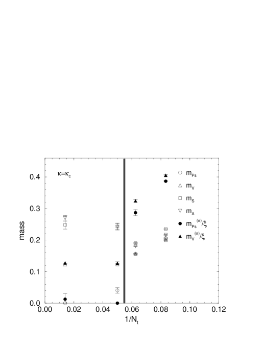
Figure 9: Temperature dependence of masses (in $a_{\tau}^{-1}$) at $\kappa_{\sigma}=0.086$ (top) and in the chiral limit (bottom). Full (open) symbols correspond to spatial (temporal) masses. The grey vertical line roughly represents $T_{c}$.

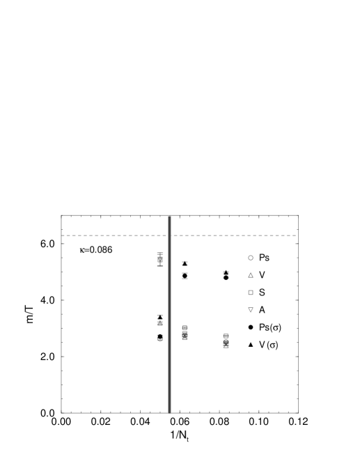
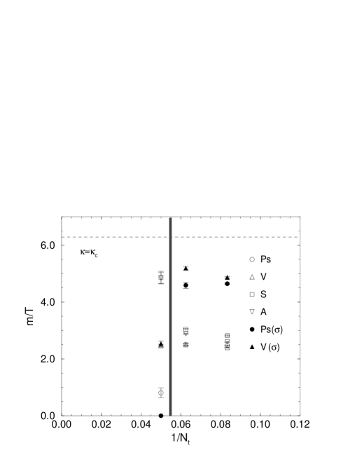
Figure 10: $m/T$ at $T\simeq 0.93\,T_{c},\,1.15\,T_{c}$ and $1.5\,T_{c}$ for $\kappa_{\sigma}=0.086$ (top) and in the chiral limit (bottom). Full (open) symbols correspond to spatial (temporal) masses. The grey vertical line roughly represents $T_{c}$. The dashed horizontal line corresponds to twice the lowest Matsubara frequency.

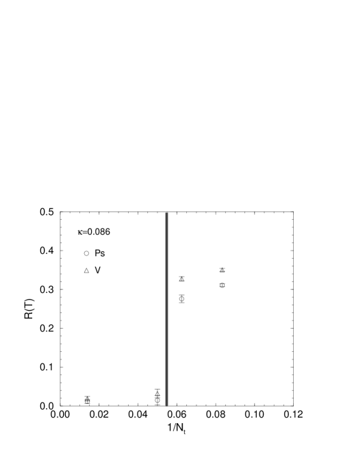
Figure 11: The phenomenological parameter $R$ eq. (38) as function of $T$. The grey vertical line roughly represents $T_{c}$.

Temperature dependence

The temperature dependence of temporal and screening masses is summarized in Fig. 9. The values are given in units of $a_{\tau}^{-1}$. The horizontal axis is $1/N_{\tau}$ and we have $T=1/N_{\tau}a_{\tau}$ with $a_{\tau}^{-1}=4.5(2)$ GeV. The four points ($N_{\tau}=72,\,20,\,16$ and $12$) correspond to the temperatures $T\simeq 0,\,0.93\,T_{c},\,1.15\,T_{c}$ and $1.5\,T_{c}$. The vertical gray line roughly corresponds to the critical temperature.

In the confining phase, the temporal and screening (spatial) masses coincide, however above $T_{c}$ they become increasingly different. This is to be expected, since the former (whether they represent bound states or not) are related to propagation in plasma with the transfer matrix of the original problem, while the latter correspond to a $T=0$ problem with asymmetric finite size effects, strongly increasing with the temperature (one of the “spatial” direction becomes squeezed as $1/T$). In agreement with other works [12], screening masses above $T_{c}$ are $\propto T$ and close to twice the lowest Matsubara frequency (the lowest quark momentum in the squeezed direction with a.p.b.c.), although remaining below it for all $T$. On Fig. 10 we plot the ratios $m/T$ for the three non-zero temperatures together with twice the lowest Matsubara frequency for comparison. The temporal masses above $T_{c}$ are also proportional with $T$ but with a significantly smaller slope. The slight decrease of the Ps and V temporal masses ($\times 1/T$) above $T_{c}$ in the upper plot of Fig. 10 is due to the large quark mass in the simulation, which produces a term $\propto 1/T$ in this plot. This decrease disappears in the chiral limit (lower plot).

As a phenomenological parameter to succinctly quantify this behavior we introduce:

$$R=\frac{m^{(\sigma)}-m^{(\tau)}}{m^{(\sigma)}+m^{(\tau)}}\ {\!\begin{array}[]{c}\vspace*{-0.2cm}{}\hfil\\ {\longrightarrow\vspace*{-0.2cm}}\\ {\scriptscriptstyle\rm P.Th.}\end{array}\!}\ 1-\frac{2m_{q}}{\pi T}+...\,,\ \ \ m_{q}\ll T\ll a_{\tau}^{-1}.$$ (38)

Since at high $T$ the quarks are expected to exhibit an effective (temporal) mass $m_{q}^{eff}\sim g^{2}T/\sqrt{6}$ [27], $R\sim 1-0.26\,g^{2}$ for $T\gg T_{c}$. From Fig. 11 we see that our data tend toward this regime but are still well below it even at $T=1.5\,T_{c}$. Notice that because of large lattice artifacts in our data mass ratios are more reliable than absolute values.

Let us note again that above $T_{c}$ all four channels show almost the same masses. In the present quenched calculation, the chiral symmetry is not involved in the dynamics and the phase transition is the deconfining transition. Nevertheless, the chiral symmetry seems to be restored, which indicates a close relation between the two viewpoints of the QCD phase transition. This agrees with the old observation that the chiral condensate also feels the deconfining transition of pure gauge theory – see, e.g., [28].

6 Conclusions and outlook

In this quenched QCD analysis the changes of the meson properties with temperature appear to be small below $T_{c}$. Above $T_{c}$ we observe apparently opposing features: On the one hand, the behavior of the $t$-propagators, in particular the change in the ordering of the mass splittings could be accounted for by contributions from free quark propagation in the mesonic channels, which would also explain the variation of $m^{(\tau)}_{eff}(t)$ both with $t$ and with the source. On the other hand, the behavior of the wave functions obtained from the 4-point correlators suggests that there can be low energy excitations in the mesonic channels above $T_{c}$ appearing as metastable bound states which replace the low temperature mesons. They would be characterized by a mass giving the location of the corresponding bump in the spectral function. In this case the variation of $m^{(\tau)}_{eff}(t)$ with $t$ and with the source would indicate a resonance width for these states, increasing with $T$. Our treatment of the low energy states using the $exp$-$exp$ source introduces, however, uncertainties which do not allow for quantitative conclusions. As we have seen this source is indeed slightly too wide and includes some contributions from excited states compensating each other in the $ee$-$pp$ correlator at $T<T_{c}$. At high $T$ the “effective” mass becomes therefore increasingly ambiguous. Remember, however, that our source is not chosen arbitrarily but selects a state according to the internal structure of the latter on the basis of the similarity with the wave function of the $T=0$ mesonic ground state. What we find is that at all temperatures there is a tendency for stable spatial correlation between quarks with a shape similar to the $T=0$ wave function. It seems therefore reasonable to hypothesize that at all temperatures this source finds a low energy mode characterized by strong, stable spatial correlations between the quarks, and that the properties of the propagators taken with this source will reflect within some uncertainties the properties of this mode.

We see clear signal for chiral symmetry restoration starting early above $T_{c}$. Since this is a quenched calculation, this effect is completely due to the gluonic dynamics. Above $T_{c}$ the screening masses increase faster than the (temporal) masses, remaining however clearly below the free gas limit. The exact amount of splitting among the channels and the precise ratio between $m^{(\tau)}$ and $m^{(\sigma)}$ may, however, be affected also by uncertainties in our $\xi$ calibration, in the definition of the source etc: Especially the temporal masses might be misestimated (if they are at all well defined). But the semi-quantitative picture of much (and, with $T$, increasingly) steeper “screening” propagators (as compared with temporal ones) is undoubtful.

A possible physical picture is this: Mesonic excitations are present above $T_{c}$ (up to at least $1.5T_{c}$) as unstable modes (resonances), in interaction with unbound quarks and gluons. They may be realized as collective states, by the interaction of the original mesons with new effective degrees of freedom in the thermal bath, or as metastable bound states (of thermal quarks?). To the extent that our results can be interpreted as supporting this picture, we should note that:

- the “temporal masses” of these putative states in the pseudo-scalar and vector channels connect smoothly to the “pole” masses of the mesons below $T_{c}$ (the S and A correlators change more significantly, in accordance with the chiral symmetry restoration),

- the increase of the temporal meson masses with $T$ is to a certain extent similar to that of the quark thermal mass if we assume $g^{2}\sim 1$ (while the spatial masses increase much faster),

- the wave functions characterizing these states are very similar to those of the genuine mesons below $T_{c}$,

- since there is no pair creation (no dynamical quarks) a “decay channel” for these putative resonances may be $meson\rightarrow q_{th}\ +\ {\bar{q}}_{th}$ where by $q_{th}\,+\,{\bar{q}}_{th}$ we indicate some strongly interacting but unbound quark states,

- the incomplete (quenched) dynamics of this simulation seems to already provide enough interaction to account (besides for mesonic states below $T_{c}$) for chiral symmetry restoration and binding forces above $T_{c}$; nevertheless effects of dynamical quarks of small enough masses may add further features to this picture.

Although our results are consistent with the above picture, there may be also other possibilities (cf [6, 7], cf [1] and references therein). We also see agreement with the earlier study of meson propagators including dynamical quarks (but without wave function information) [7], which finds masses and (spatial) screening masses $\propto T$ above $T_{c}$ and indication for QGP with “deconfined, but strongly interacting quarks and gluons”. Investigations of mesonic correlation functions in HTL approximation [24] show that the observed effects cannot be reproduced from perturbative thermal physics. The wave function analysis in our work indicates in fact that the strong interactions between the thermal gluons and quarks may even provide binding forces which partially correlate the latter in space.

The complex, non-perturbative structure of QGP (already indicated by equation of state studies up to far above $T_{c}$ [10], see also [29]) is thus also confirmed by our analysis of general mesonic correlators. From our more extended study however, especially from the, here for the first time investigated, spatial correlations between quarks propagating in the temporal direction at $T>T_{c}$ (wave functions), the detailed low energy structure of the mesonic channels appears to present further interesting, yet unsolved aspects and therefore provide an exciting and far from trivial picture of QGP in the region up to (at least) $1.5T_{c}$. Further work is needed to remove the uncertainties still affecting our analysis. This concerns particularly the $\xi$ calibration and the question of the definition of hadron operators at high $T$, which appear to have been the major deficiencies, besides the smaller lattices, affecting earlier results [17]. We are also trying to extract information directly about the spectral functions [30]. Finally we are aiming at performing a full QCD analysis in the near future.

Acknowledgments: We thank JSPS, DFG and the European Network “Finite Temperature Phase Transitions in Particle Physics” for support. H.M. thanks T. Kunihiro and H. Suganuma and I.O.S. thanks F. Karsch and J. Stachel for interesting discussions. H.M. also thank the Japan Society for the Promotion of Science for Young Scientists for financial support. O.M. and A.N. were supported by the Grant-in-Aide for Scientific Research by the Ministry of Education and Culture, Japan (No.80029511) and A.N. was also supported by the Grant-in-Aide (No.10640272). M.G.P. was supported by CICYT under grant AEN97-1678. The calculations have been done on the AP1000 at Fujitsu Parallel Comp. Res. Facilities and the Intel Paragon at the Institute for Nonlinear Science and Applied Mathematics, Hiroshima University.

Appendix: Calibration of anisotropy parameters

To determine the gauge field anisotropy $\xi$, we use the ratios of the spatial-spatial and spatial-temporal Wilson loops [31, 32, 33]:

$$R_{\sigma}(r,x) = W_{\sigma\sigma}(r+1,x)/W_{\sigma\sigma}(r,x),$$

$$R_{\tau}(r,t) = W_{\sigma\tau}(r+1,t)/W_{\sigma\tau}(r,t).$$ (39)

Then the matching condition (34) is

$$R_{\sigma}(r,x)=R_{\tau}(r,t=\xi\,x).$$ (40)

80 configurations are used for this analysis.

In the determination of $\xi$, we vary the minimum value of $r\times x$ (with corresponding choice of $t$), where $r\leq 5$ ($r=1$ and $x=1$ are not used to avoid short distance effects). The largest value of $x$ for each $r$ is chosen with consideration to the statistical errors. We obtain $\xi=5.397(22)$ ($r\times x\geq 4$), $5.340(40)$ ($r\times x\geq 6$), $5.248(101)$ ($r\times x\geq 8$) and take therefore $\xi=5.3(1)$ in the following.

To determine the lattice spacings, the heavy quark potential is measured. The extracted value of the string tension $\sqrt{\sigma}=0.480(23)$ together with physical value $\sqrt{\sigma_{phys}}=427$ MeV gives the cutoffs $a_{\sigma}^{-1}=0.85(3)$ GeV and $a_{\tau}^{-1}=4.5(2)$ GeV. The spatial extent of the lattice of about 3 fm ($\sim 4$ times $1/T_{c}$) is considered sufficiently large to treat hadronic correlators.

We then proceed to the fermionic calibration. We fix the value of $\kappa_{\sigma}$ and vary $\gamma_{F}$ to find out the value which gives the same anisotropy $\xi$ as for the gauge field. We define the fermionic anisotropy using correlators in temporal and spatial directions, expected to behave at large distances like

$$G_{\tau,M}^{(pp\rightarrow pp)}(t)=\langle\Phi_{M}^{(pp)}(t)\,\Phi_{M}^{(pp)}(0)^{{\dagger}}\rangle{\!\begin{array}[]{c}\vspace*{-0.2cm}{}\hfil\\ {\longrightarrow\vspace*{-0.2cm}}\\ {\scriptscriptstyle t\rightarrow\infty}\end{array}\!}C_{\gamma}^{(\tau)}\,\exp(-m_{M}^{(\tau)}t)$$ (41)

and the same expression with time replaced by one of the spatial directions $z$, behaving as $C_{\gamma}^{(\sigma)}\,\exp(-m_{M}^{(\sigma)}z)$ for large $z$.

In the calibration, we measure the pseudo-scalar ($\gamma_{\rm M}=\gamma_{5}$) and the vector ($\gamma_{1}$, $\gamma_{2}$) meson correlators. Here we adopt anti-periodic boundary conditions in all four directions, hence the expected behavior is a hyperbolic cosine. The physical isotropy condition (34) is then applied to the effective masses. Figure 12 shows $m^{(\tau)}_{eff}(t)$ obtained by solving (28) and the corresponding $m^{(\sigma)}_{eff}(z)$ for $\kappa_{s}=0.081$ and with two values of $\gamma_{F}$. On the figure $m^{(\sigma)}_{eff}(z)$ is divided by $\xi=5.3$ to be compared with $m^{(\tau)}_{eff}(t)$ (i.e., it is given in units $a_{\tau}^{-1}$).

For $\gamma_{F}=4.05$, the spatial effective mass divided by $\xi=5.3$ coincides with the temporal one. Although the former shows no plateau because of the small number of spatial sites, the temporal effective mass, which is finer spaced, does reach a plateau in the large $t$ region. It is consistent to expect that if both masses agree (after $\xi-$rescaling) in the region where the temporal mass shows a plateau, the spatial mass is also dominated by the ground state. We therefore determine $\xi_{F}$, the fermionic anisotropy, as the ratio of the spatial effective mass at $z=5$ and the fitted value of the temporal mass in the interval $t=27$-$36$. The value of $\xi_{F}$ and the extracted masses are confirmed by studying correlators with smeared operators which do reach plateaus much earlier. The smearing procedure of the correlators in the temporal direction is described in detail in the next section. For the correlators in spatial directions, we apply the gauge invariant smearing technique [26] (since the configurations are fixed to the Coulomb gauge).

Though these calculations are carried out with periodic boundary conditions in spatial directions, the dependence of masses on the kind of boundary conditions is sufficiently small on the present lattice.

Figure 13 shows the dependence of $\xi_{F}$ on $\gamma_{F}$. The values of $\xi_{F}$ from Ps and V mesons are slightly different, but consistent within the present accuracy. We adopt the averaged value of Ps and V channels and estimate the error as their difference.

We use three sets of ($\kappa_{\sigma}$, $\gamma_{F}$): (0.081, 4.05), (0.084, 3.89) and (0.086, 3.78). In Table 1, these values are listed together with the number of configurations used for calibration. For the second set, two values of $\gamma_{F}$ are tried. The meson masses quoted in the table are determined in section 4 using smeared correlators.

Another procedure to calibrate the fermionic action using the dispersion relation is proposed in [34]. In the present case, however, the procedure used above seems more appropriate, since comparison of pole and screening masses at finite temperature is one of the important goals of this work.

Figure 12: The effective masses of correlators in temporal and spatial directions for $\kappa_{\sigma}=0.081$ with two values of $\gamma_{F}$, 4.02 and 4.05.

Figure 13: $\xi_{F}$’s determined from the Ps and V correlators for $\kappa_{\sigma}=0.081$ with various values of $\gamma_{F}$.

References

- [1] H. Meyer-Ortmanns, Rev. Mod. Phys. 68 (1996) 473.
- [2] H. Satz, hep-ph/9706342, “QCD and QGP: a summary”; hep-ph/9711289, “Color deconfinement and J/Psi suppression in high-energy nuclear collisions”.
- [3] R. Rapp and W. Gale, Phys. Rev. C60 (1999) 024903; G.E. Brown, G.Q. Li, R. Rapp, M, Rho, J. Wambach, Acta. Phys. Polon. B29 (1998) 2309.
- [4] T. Hatsuda and T. Kunihiro, Phys. Rep. 247 (1994) 221.
- [5] S. Gottlieb et al., Phys. Rev. Lett. 59 (1987) 2247, Phys. Rev. D 38 (1988) 2888; S. Gottlieb et al., Phys. Rev. D 55 (1997) 6852.
- [6] C. DeTar, Phys. Rev. D 32 (1985) 276; 37 (1988) 2328.
- [7] G. Boyd, S. Gupta, F. Karsch, E. Laermann, Z. f. Physik C 64 (1994) 331.
- [8] P. Braun-Munzinger, I. Heppe and J. Stachel, Phys. Lett. B465 (1999) 15; J. Stachel, Nucl. Phys. A654 (1999) 119c.
- [9] CERN Press Release 2000.02.10.: “A New State of Matter created at CERN”.
- [10] F. Karsch, Nucl. Phys. B (Proc. Suppl.) 83-84 (2000) 14; hep-lat/9903031, “Deconfinement and chiral symmetry restoration”.
- [11] E. Laermann, Nucl. Phys. B (Proc. Suppl.) 63A-C (1998) 114.
- [12] C. Bernard et al., Phys. Rev. Lett. 68 (1992) 2125; F. Karsch, Nucl. Phys. B (Proc. Suppl.) 34 (1994) 63; P. Schmidt and E. Laermann, Nucl. Phys. B (Proc. Suppl.) 63A-C (1998) 391.
- [13] E. Laermann et al., Nucl. Phys. B (Proc. Suppl.) 34 (1994) 292; J.-F. Lagae, D.KJ.Sinclair, J.B. Kogut, hep-lat/9806001, “Thermodynamics of lattice QCD with 2 quark flavors: chiral symmetry and topology”.
- [14] For a review, see e.g. N.P. Landsman and Ch.G. van Weert, Phys. Rep. 145 (1987) 141.
- [15] A.A. Abrikosov, L.P. Gor’kov and I.E. Dzyaloshinskii, Sov. Phys. JETP 36(9) (1959) 636; E.S. Fradkin, ibid. 912.
- [16] J. Engels, F. Karsch and H. Satz, Nucl. Phys. B205[FS5] (1982) 239.
- [17] T. Hashimoto, A. Nakamura and I.-O. Stamatescu, Nucl. Phys. B 400 (1993) 267.
- [18] T. Hashimoto, A. Nakamura and I.-O. Stamatescu, Nucl. Phys. B 406 (1993) 325.
- [19] F. Karsch, Nucl. Phys. B 205 (1982) 285.
- [20] H. Narnhofer, M. Requardt and W. Thirring, Commun. Math. Phys. 92 (1983) 247.
- [21] G. Burgers et al. Nucl. Phys. B304 (1988) 587.
- [22] QCD-TARO Collaboration (Ph. de Forcrand et al.), Nucl. Phys. B (Proc. Suppl.) 73 (1999) 420; hep-lat/9901017, “Mesons Above The Deconfining Transition” (unpublished).
- [23] QCD-TARO Collaboration (M. Fujisaki et al.), Nucl. Phys. B (Proc.Suppl.) 53 (1997) 426.
- [24] F. Karsch, M.G. Mustafa, M.H. Thoma, hep-ph/0007093, “Finite temperature meson correlation functions in HTL approximation”.
- [25] D. Weingarten, Phys. Rev. Lett. 51 (1983) 1830.
- [26] S. Güsken et al., Phys. Lett. B 227 (1989) 266.
- [27] G. Boyd, Sourendu Gupta and F. Karsch, Nucl. Phys. B385 (1992) 481.
- [28] J. Kogut et al., Nucl. Phys. B225 (1983) 326.
- [29] G. Boyd et al., Nucl. Phys. B 469 (1996) 419.
- [30] QCD-TARO Collaboration (Ph. de Forcrand et al.), Nucl. Phys. B (Proc. Suppl.) 63 (1998) 460; TARO, work in progress.
- [31] QCD-TARO Collaboration (M. Fujisaki et al.), Nucl. Phys. B (Proc. Suppl.) 53 (1997) 426; in Vol. Multi-scale Phenomena and their Simulation, F.Karsch, B.Monien and H.Satz eds., World Scientific (Singapore 1997) 208.
- [32] J. Engels, F. Karsch and T. Scheideler, Nucl. Phys. B (Proc. Suppl.) 63 A-C (1998) 427.
- [33] T.R. Klassen, Nucl. Phys. B 533 (1998) 557.
- [34] T.R. Klassen, Nucl. Phys. B (Proc. Suppl.) 73 (1999) 918.