Topology and metastability in the lattice Skyrme model

Abstract

We offer the Skyrme model on a lattice as an effective field theory—fully quantized—of baryon–meson interactions at temperatures below the chiral phase transition. We define a local topological density that involves the volumes of tetrahedra in the target space $S^{3}$ and we make use of Coxeter’s formula for the Schläfli function to implement it. This permits us to calculate the mean-square radius of a skyrmion in the three-dimensional lattice Skyrme model, which may be viewed as a Ginzburg-Landau effective theory for the full quantum theory at finite temperature. We find that, contrary to expectations, the skyrmion shrinks as quantum and thermal fluctuations are enhanced. We ascribe this to a large number of metastable states that become accessible as the temperature is raised.

I Introduction

The Skyrme model [1, 2, 3, 4, 5] is a popular model of the dynamics of pions and nucleons, incorporating the former as its fundamental, pseudo-Goldstone field and the latter as topological solitons. The continuum theory has been widely studied via semiclassical techniques, giving a satisfactory phenomenology of low-momentum and low-temperature physics. In this paper we develop a lattice formulation of the model.

Our motivation in employing a lattice cutoff is to overcome the limitations of the continuum theory. In point of fact, the term “continuum theory” is misleading. The Skyrme Lagrangian is a non-linear sigma model with a four-derivative term, which makes it non-renormalizable in perturbation theory. This means that calculations of quantum effects must involve a short-distance cutoff. In working with chiral Lagrangians coupled to a local nucleon field, this is not a serious problem [8, 9, 10]. One absorbs divergences into an ever-lengthening list of counterterms; as long as external momenta are kept small, dimensional analysis limits the contributions of these counterterms to the results. When the nucleon is a soliton rather than a fundamental field, however, things are more difficult. The soliton’s collective degrees of freedom are quantized separately, and the systematic development of higher-order quantum effects involves disentangling the pion field from these collective quanta [11]. In any case, there is no way to limit the addition of higher-dimension terms to the Lagrangian as long as one must consider energy scales approaching the nucleon mass.

We propose to turn these points to advantage, by considering the Skyrme model as an effective field theory. The cutoff, and the cutoff scheme (the lattice), are part and parcel of the specification of the theory. The free choice of terms in the Lagrangian is now a virtue, constrained only by phenomenological necessity. The procedure will be to pick a Lagrangian; to fix the lattice spacing; and finally to calculate any physical quantity of interest, going beyond perturbation theory and beyond semiclassical methods, since the lattice offers many more direct techniques. From a lattice point of view, the fixed cutoff is a virtue as well, since no continuum limit is necessary (nor is it possible).

The most interesting feature of the Skyrme model is the stability conferred on the soliton by the topological conservation law and the four-derivative coupling. We wish in fact to isolate a single skyrmion in order to see how its properties change with temperature, density, etc. A recurring problem in lattice studies of solitons is the tendency of lattice dislocations to destroy topological stability or, in other words, to allow topology to slip through the lattice. We avoid this problem by choosing a lattice action that enforces continuity at short distances. In order to keep our numerical evolution within a single topological sector, we insist on a local updating scheme that should not nucleate smooth skyrmions. We find that these two ingredients suffice to stabilize the lattice skyrmion.

The main technical development in this paper is the construction of an exact topological density that can be measured on a lattice field configuration. By “exact” we mean that the winding number, the sum of the density over the lattice, is always an integer. We cut the lattice into fundamental tetrahedra and map each tetrahedron into a curved tetrahedron in the $S^{3}$ target space. The winding number is then the sum of the signed volumes of the tetrahedra in $S^{3}$. We calculate the volume of a spherical tetrahedron via a formula due to Coxeter [12], derived as a solution of differential equations first written down by Schläfli [13].

We summarize the continuum Skyrme model in Sec. II in order to establish notation. General considerations regarding continuity and topology on the lattice are presented in Sec. III, which concludes with formulae for the lattice action we employ. In Sec. IV we present our definition of the local topological density via Coxeter’s formula for the volume of a quadrirectangular tetrahedron in $S^{3}$. As a first application, we present in Sec. V the results of Monte Carlo simulation for the classical Skyrme model in three dimensions. Easier to simulate than the full four-dimensional path integral, this model may be regarded as a Ginzburg-Landau theory for the Skyrme model at finite temperature—a sort of effective theory for the effective theory. We use the topological density to calculate the mean-square radius of a skyrmion as a function of the couplings $\beta_{1}$ and $\beta_{2}$ of the lattice action. If we fix $\beta_{2}/\beta_{1}$, so that the form of the action is fixed, we find a multitude of metastable configurations of the skyrmion that are smaller than the ground state solution. As the “temperature” is raised by decreasing $\beta_{1}$ and $\beta_{2}$, these metastable states are made accessible to fluctuations, with the result that the skyrmion shrinks as it is “heated.” Presumably the “temperature” of the 3d theory is an increasing function of the real temperature in the 4d theory that it approximates. Thus we reach the result that a quantized skyrmion shrinks as it is heated.

II Continuum Skyrme model

The Euclidean action of the Skyrme model is

$$S=\int d^{4}x\left[\frac{f_{\pi}^{2}}{16}\mathop{\text{Tr}}|\partial_{\mu}U|^{2}+\frac{1}{32e^{2}}\mathop{\text{Tr}}([L_{\mu},L_{\nu}])^{2}\right],$$ (1)

where the non-linear chiral field $U$ is an $SU(2)$ matrix, and we have defined

$$L_{\mu}=iU^{{\dagger}}\partial_{\mu}U.$$ (2)

We have omitted a mass term of the form $m_{\pi}^{2}\mathop{\text{Tr}}U$ and thus $S$ is invariant under the $SU(2)\times SU(2)$ group of chiral rotations,

$$U\to AUB^{{\dagger}},\text{ with }A,B\in SU(2).$$ (3)

Classically, the symmetry is spontaneously broken. Finite-energy field configurations must tend to a constant at infinity, and one can use a symmetry rotation to make this constant the unit matrix, i.e.,

$$U({\bf x})\to\openone\text{ as }|{\bf x}|\to\infty.$$ (4)

Using the Pauli matrices $\tau_{i}$, $i=1,2,3$, we can write $U$ in terms of new fields $\mathchoice{{\hbox{\boldmath$\displaystyle\sigma$}}}{{\hbox{\boldmath$\textstyle\sigma$}}}{{\hbox{\boldmath$\scriptstyle\sigma$}}}{{\hbox{\boldmath$\scriptscriptstyle\sigma$}}}=(\sigma_{0},\sigma_{i})$ via

$$U=\sigma_{0}+i\sigma_{i}\tau_{i},$$ (5)

where $\mathchoice{{\hbox{\boldmath$\displaystyle\sigma$}}}{{\hbox{\boldmath$\textstyle\sigma$}}}{{\hbox{\boldmath$\scriptstyle\sigma$}}}{{\hbox{\boldmath$\scriptscriptstyle\sigma$}}}\cdot\mathchoice{{\hbox{\boldmath$\displaystyle\sigma$}}}{{\hbox{\boldmath$\textstyle\sigma$}}}{{\hbox{\boldmath$\scriptstyle\sigma$}}}{{\hbox{\boldmath$\scriptscriptstyle\sigma$}}}=1$. By considering small fluctuations about $U=\openone$, we can identify $\sigma_{i}$, $i=1,2,3$ with the Goldstone pion field.

Equation (4) means that 3-dimensional space is compactified to the 3-sphere $S^{3}$. Since $U\in SU(2)$ also takes values in $S^{3}$ [see Eq. (5)], configurations $U({\bf x})$ can be classified according to the homotopy group $\pi_{3}(S^{3})=Z$. Thus there is an integer winding number $n$ that denotes how many times $U({\bf x})$ covers the 3-sphere in field space as x is varied over its 3-sphere. This winding number is topologically conserved, meaning that it cannot change under continuous deformation of the field $U({\bf x})$.

The $n=0$ sector includes the vacuum $U({\bf x})=\openone$ and perturbations around it. An example of an $n=1$ configuration is the spherically symmetric skyrmion,

$$U({\bf x})=\exp\left[if(r)\frac{x_{i}\tau_{i}}{r}\right],$$ (6)

with

$$f(0) = \pi,$$ (7)

$$f(\infty) = 0.$$ (8)

$f(r)$ should be determined so as to minimize the static energy

$$E=\int d{\bf x}\left[\frac{f_{\pi}^{2}}{16}\mathop{\text{Tr}}|\partial_{i}U|^{2}+\frac{1}{32e^{2}}\mathop{\text{Tr}}([L_{i},L_{j}])^{2}\right],$$ (9)

but a simple choice with the right topology is

$$f(r)=\pi\left(1-\tanh\frac{r}{r_{0}}\right).$$ (10)

Skyrme identified $n$ with the baryon number of a field configuration, and the lowest soliton configuration with the nucleon.

Given an arbitrary field configuration $U({\bf x})$ satisfying Eq. (4), its winding number may be calculated with the formula

$$n=\frac{i}{24\pi^{2}}\int d{\bf x}\,\epsilon_{ijk}\mathop{\text{Tr}}L_{i}L_{j}L_{k}.$$ (11)

The geometric meaning of Eq. (11) will be apparent in its lattice counterpart below.

III Lattice topology and continuity

In this section we define a topological density for a lattice field configuration that is unambiguous and that sums exactly to an integer. The further demand of conservation of the winding number will lead us to choosing a lattice action that constrains discontinuities in the field.

A lattice configuration is specified by the field $U_{\bf n}\in SU(2)$ or, equivalently, by the 4-vector $\mathchoice{{\hbox{\boldmath$\displaystyle\sigma$}}}{{\hbox{\boldmath$\textstyle\sigma$}}}{{\hbox{\boldmath$\scriptstyle\sigma$}}}{{\hbox{\boldmath$\scriptscriptstyle\sigma$}}}_{\bf n}\in S^{3}$. In order to define the winding number, we begin [7] by cutting the cubic lattice $L^{3}$ into tetrahedra, five tetrahedra per cubic cell (see Fig. 1).

FIG. 1.: A cube cut into 5 tetrahedra. The even vertices (circled) are connected to form a central tetrahedron and four others. In neighboring cubes, the odd vertices are to be connected instead, so that the diagonal edges match up.

The four vertices ${\bf n}^{(i)}$, $i=1$–4 of each tetrahedron map to four unit 4-vectors $\mathchoice{{\hbox{\boldmath$\displaystyle\sigma$}}}{{\hbox{\boldmath$\textstyle\sigma$}}}{{\hbox{\boldmath$\scriptstyle\sigma$}}}{{\hbox{\boldmath$\scriptscriptstyle\sigma$}}}^{(i)}$, which are vertices of a spherical tetrahedron in $S^{3}$. This tetrahedron is defined via its vertices; its edges are arcs of great circles and its faces are spherical triangles drawn on great spheres.

Since three (non-collinear) points in $S^{3}$ determine a great sphere, it is clear that two adjacent tetrahedra in $L^{3}$ map into adjacent tetrahedra in $S^{3}$, with the common face in $L^{3}$ mapping into a common face in $S^{3}$. Thus the field configuration $\mathchoice{{\hbox{\boldmath$\displaystyle\sigma$}}}{{\hbox{\boldmath$\textstyle\sigma$}}}{{\hbox{\boldmath$\scriptstyle\sigma$}}}{{\hbox{\boldmath$\scriptscriptstyle\sigma$}}}_{\bf n}$ gives a triangulation of some volume in $S^{3}$. We impose periodic boundary conditions on the lattice, and thus no tetrahedron possesses a face that is not shared by another tetrahedron (a free face). This implies that the complex of tetrahedra in $S^{3}$ possesses no free faces either, and thus the volume covered by the complex must be an integer multiple of the volume of $S^{3}$. If the field configuration is smooth, the complex in $S^{3}$ will be composed of tetrahedra that are small compared to $S^{3}$, and it will wrap around the sphere much as a smooth mapping of the 3-torus must. In any case, the volume in $S^{3}$ of the five tetrahedra corresponding to a cube in $L^{3}$ gives a definition of the topological density $\rho_{\bf n}$ contained in the cube.

The topological density thus defined is not unambiguous, however. If a tetrahedron in $S^{3}$ is specified by its faces, then there are two volumes in $S^{3}$ that are bounded by these faces. One of the volumes includes the north pole (for example), and the other does not. If one of the volumes is measured to be a positive $V$ (with $V<1$), then the other volume will be $V-1$. (Careful attention to the orientation will make the latter negative.) In order to assign a unique topological density to a lattice field configuration, we define a tetrahedron’s volume to satisfy $|V|<\frac{1}{2}$.

We have solved the problem of uniqueness, but not that of conservation of the winding number. Consider a field configuration wherein one tetrahedron in $S^{3}$ has volume $\frac{1}{2}-\epsilon$, where $\epsilon$ is small. Under a fluctuation of one of the vertices of the tetrahedron, its volume may shift to $\frac{1}{2}+\delta$, while the neighboring tetrahedra change their volumes by $-(\epsilon+\delta)$ so that the winding number is unchanged. Unfortunately, our algorithm will now redefine the volume of the first tetrahedron to $-\frac{1}{2}+\delta$, resulting in a loss of 1 in the winding number. This is often called “topology dropping through the lattice.”

The procedure to be followed at this point depends on the physics to be investigated. One might want to study, for example, the thermodynamics of the Skyrme model by fixing a chemical potential $\mu$ coupled to the winding number. The grand partition function would then be

$$Z(\mu)=\sum_{n}e^{\mu n}Z_{n},$$ (12)

where $Z_{n}$ is a sum over all field configurations with winding number $n$. A Monte Carlo simulation should then be allowed to wander freely among the sectors of different $n$, subject to an acceptance/rejection test that enforces the relative probabilities $e^{\mu n}$. A local updating algorithm can nucleate “point skyrmions” as in the preceding paragraph, which change $n$ by a unit and then spread out into smoother skyrmions; in addition, a non-local update could be permitted that creates smooth skyrmions directly.

Our interest, however, is in the properties of a single skyrmion, which are accessible through a canonical ensemble at fixed $n=1$. The simulation must be constrained so as not to change $n$. This requires that we prevent the nucleation of both point skyrmions and smooth skyrmions. The latter can be prevented by choosing a local updating algorithm. For the former, we choose a lattice action that excludes the possibility of tetrahedra in $S^{3}$ with $|V|\approx\frac{1}{2}$. We adopt the kinetic term [14]

$$S_{1}=(\alpha-1)\sum_{{\bf n}\mu}\log(\mathchoice{{\hbox{\boldmath$\displaystyle\sigma$}}}{{\hbox{\boldmath$\textstyle\sigma$}}}{{\hbox{\boldmath$\scriptstyle\sigma$}}}{{\hbox{\boldmath$\scriptscriptstyle\sigma$}}}_{\bf n}\cdot\mathchoice{{\hbox{\boldmath$\displaystyle\sigma$}}}{{\hbox{\boldmath$\textstyle\sigma$}}}{{\hbox{\boldmath$\scriptstyle\sigma$}}}{{\hbox{\boldmath$\scriptscriptstyle\sigma$}}}_{{\bf n}+{\hat{\mu}}}-\alpha)$$ (13)

in order to constrain $\mathchoice{{\hbox{\boldmath$\displaystyle\sigma$}}}{{\hbox{\boldmath$\textstyle\sigma$}}}{{\hbox{\boldmath$\scriptstyle\sigma$}}}{{\hbox{\boldmath$\scriptscriptstyle\sigma$}}}_{\bf n}\cdot\mathchoice{{\hbox{\boldmath$\displaystyle\sigma$}}}{{\hbox{\boldmath$\textstyle\sigma$}}}{{\hbox{\boldmath$\scriptstyle\sigma$}}}{{\hbox{\boldmath$\scriptscriptstyle\sigma$}}}_{{\bf n}+{\hat{\mu}}}>\alpha$ and thus to reject fluctuations that put large angles between neighboring field variables. With some Monte Carlo exploration, we can find a value of $\alpha$ that will keep the tetrahedral volumes far enough from $\frac{1}{2}$.

For smooth configurations, we expand $\mathchoice{{\hbox{\boldmath$\displaystyle\sigma$}}}{{\hbox{\boldmath$\textstyle\sigma$}}}{{\hbox{\boldmath$\scriptstyle\sigma$}}}{{\hbox{\boldmath$\scriptscriptstyle\sigma$}}}_{\bf n}\cdot\mathchoice{{\hbox{\boldmath$\displaystyle\sigma$}}}{{\hbox{\boldmath$\textstyle\sigma$}}}{{\hbox{\boldmath$\scriptstyle\sigma$}}}{{\hbox{\boldmath$\scriptscriptstyle\sigma$}}}_{{\bf n}+{\hat{\mu}}}$ around 1 and Eq. (13) becomes

$$S_{1} \simeq \sum_{{\bf n}\mu}(1-\mathchoice{{\hbox{\boldmath$\displaystyle\sigma$}}}{{\hbox{\boldmath$\textstyle\sigma$}}}{{\hbox{\boldmath$\scriptstyle\sigma$}}}{{\hbox{\boldmath$\scriptscriptstyle\sigma$}}}_{\bf n}\cdot\mathchoice{{\hbox{\boldmath$\displaystyle\sigma$}}}{{\hbox{\boldmath$\textstyle\sigma$}}}{{\hbox{\boldmath$\scriptstyle\sigma$}}}{{\hbox{\boldmath$\scriptscriptstyle\sigma$}}}_{{\bf n}+{\hat{\mu}}})$$ (14)

$$= \sum_{{\bf n}\mu}\left[1-\frac{1}{2}\text{Tr}\,\left(U_{\bf n}U_{{\bf n}+{\hat{\mu}}}^{{\dagger}}\right)\right]$$ (15)

$$= \sum_{{\bf n}\mu}\frac{1}{4}\text{Tr}\,\left(U_{{\bf n}+{\hat{\mu}}}-U_{\bf n}\right)\left(U_{{\bf n}+{\hat{\mu}}}^{{\dagger}}-U_{\bf n}^{{\dagger}}\right),$$ (16)

which approaches the kinetic term in Eq. (1) in the continuum limit.

A technical point remains. We have discussed the ambiguity in fixing the volume of a tetrahedron if its faces are given, which led us to require $|V|<\frac{1}{2}$. A lattice field configuration $\mathchoice{{\hbox{\boldmath$\displaystyle\sigma$}}}{{\hbox{\boldmath$\textstyle\sigma$}}}{{\hbox{\boldmath$\scriptstyle\sigma$}}}{{\hbox{\boldmath$\scriptscriptstyle\sigma$}}}_{\bf n}$ gives us only the vertices of each tetrahedron, however, not its faces. Given three vertices that determine a great sphere, the face that connects them can be chosen to be either of two triangles that together make up the sphere. A little thought shows that the difference between the volumes enclosed is $\frac{1}{2}$. This gives an ambiguity between a value $V>0$ and $V-\frac{1}{2}$ for the volume of the tetrahedron.

This last ambiguity involves choosing which triangle constitutes the face of the tetrahedron. But this face is shared between two adjacent tetrahedra, and the ambiguity will be immaterial if the same choice is made for both. This is hard to program, however, if each tetrahedron is to be handled on its own. We prefer to resolve the ambiguity for each tetrahedron separately, by requiring that $|V|<\frac{1}{4}$. We impose this via a more restrictive choice of $\alpha$ in Eq. (13). We find that setting $\alpha=0.1$ is adequate for the purpose.

A local updating algorithm based on the action (13) will conserve winding number. Even so, a skyrmion will tend to shrink down to a point in accordance with the scaling argument that gives Derrick’s Theorem. This is because the stabilization is being done at the scale of a single lattice spacing; only here will the scaling argument fail and the skyrmion run into a repulsive potential. In order to have a stable skyrmion of appreciable size, we cannot avoid adding a Skyrme term as in Eq. (1). The most straightforward lattice transcription uses symmetric derivatives [6],

$$S_{2}^{\text{SYM}}=\sum_{\bf n}\sum_{\mu>\nu}\left\{\left(\mathchoice{{\hbox{\boldmath$\displaystyle\sigma$}}}{{\hbox{\boldmath$\textstyle\sigma$}}}{{\hbox{\boldmath$\scriptstyle\sigma$}}}{{\hbox{\boldmath$\scriptscriptstyle\sigma$}}}_{{\bf n}+{\hat{\mu}}}-\mathchoice{{\hbox{\boldmath$\displaystyle\sigma$}}}{{\hbox{\boldmath$\textstyle\sigma$}}}{{\hbox{\boldmath$\scriptstyle\sigma$}}}{{\hbox{\boldmath$\scriptscriptstyle\sigma$}}}_{{\bf n}-{\hat{\mu}}}\right)^{2}\left(\mathchoice{{\hbox{\boldmath$\displaystyle\sigma$}}}{{\hbox{\boldmath$\textstyle\sigma$}}}{{\hbox{\boldmath$\scriptstyle\sigma$}}}{{\hbox{\boldmath$\scriptscriptstyle\sigma$}}}_{{\bf n}+{\hat{\nu}}}-\mathchoice{{\hbox{\boldmath$\displaystyle\sigma$}}}{{\hbox{\boldmath$\textstyle\sigma$}}}{{\hbox{\boldmath$\scriptstyle\sigma$}}}{{\hbox{\boldmath$\scriptscriptstyle\sigma$}}}_{{\bf n}-{\hat{\nu}}}\right)^{2}-\left[\left(\mathchoice{{\hbox{\boldmath$\displaystyle\sigma$}}}{{\hbox{\boldmath$\textstyle\sigma$}}}{{\hbox{\boldmath$\scriptstyle\sigma$}}}{{\hbox{\boldmath$\scriptscriptstyle\sigma$}}}_{{\bf n}+{\hat{\mu}}}-\mathchoice{{\hbox{\boldmath$\displaystyle\sigma$}}}{{\hbox{\boldmath$\textstyle\sigma$}}}{{\hbox{\boldmath$\scriptstyle\sigma$}}}{{\hbox{\boldmath$\scriptscriptstyle\sigma$}}}_{{\bf n}-{\hat{\mu}}}\right)\cdot\left(\mathchoice{{\hbox{\boldmath$\displaystyle\sigma$}}}{{\hbox{\boldmath$\textstyle\sigma$}}}{{\hbox{\boldmath$\scriptstyle\sigma$}}}{{\hbox{\boldmath$\scriptscriptstyle\sigma$}}}_{{\bf n}+{\hat{\nu}}}-\mathchoice{{\hbox{\boldmath$\displaystyle\sigma$}}}{{\hbox{\boldmath$\textstyle\sigma$}}}{{\hbox{\boldmath$\scriptstyle\sigma$}}}{{\hbox{\boldmath$\scriptscriptstyle\sigma$}}}_{{\bf n}-{\hat{\nu}}}\right)\right]^{2}\right\}.$$ (17)

This couples each site to sites two links away, effectively via plaquette couplings across plaquettes of side $\sqrt{2}$, and fails to couple the odd and even sublattices. We prefer to use a discretization [15] that couples only across single plaquettes, of side 1:

$$S_{2}=4\sum_{\bf n}\sum_{\mu>\nu}\left\{\left(\mathchoice{{\hbox{\boldmath$\displaystyle\sigma$}}}{{\hbox{\boldmath$\textstyle\sigma$}}}{{\hbox{\boldmath$\scriptstyle\sigma$}}}{{\hbox{\boldmath$\scriptscriptstyle\sigma$}}}_{{\bf n}+{\hat{\mu}}}-\mathchoice{{\hbox{\boldmath$\displaystyle\sigma$}}}{{\hbox{\boldmath$\textstyle\sigma$}}}{{\hbox{\boldmath$\scriptstyle\sigma$}}}{{\hbox{\boldmath$\scriptscriptstyle\sigma$}}}_{{\bf n}+{\hat{\nu}}}\right)^{2}\left(\mathchoice{{\hbox{\boldmath$\displaystyle\sigma$}}}{{\hbox{\boldmath$\textstyle\sigma$}}}{{\hbox{\boldmath$\scriptstyle\sigma$}}}{{\hbox{\boldmath$\scriptscriptstyle\sigma$}}}_{{\bf n}+{\hat{\mu}}+{\hat{\nu}}}-\mathchoice{{\hbox{\boldmath$\displaystyle\sigma$}}}{{\hbox{\boldmath$\textstyle\sigma$}}}{{\hbox{\boldmath$\scriptstyle\sigma$}}}{{\hbox{\boldmath$\scriptscriptstyle\sigma$}}}_{{\bf n}}\right)^{2}-\left[\left(\mathchoice{{\hbox{\boldmath$\displaystyle\sigma$}}}{{\hbox{\boldmath$\textstyle\sigma$}}}{{\hbox{\boldmath$\scriptstyle\sigma$}}}{{\hbox{\boldmath$\scriptscriptstyle\sigma$}}}_{{\bf n}+{\hat{\mu}}}-\mathchoice{{\hbox{\boldmath$\displaystyle\sigma$}}}{{\hbox{\boldmath$\textstyle\sigma$}}}{{\hbox{\boldmath$\scriptstyle\sigma$}}}{{\hbox{\boldmath$\scriptscriptstyle\sigma$}}}_{{\bf n}+{\hat{\nu}}}\right)\cdot\left(\mathchoice{{\hbox{\boldmath$\displaystyle\sigma$}}}{{\hbox{\boldmath$\textstyle\sigma$}}}{{\hbox{\boldmath$\scriptstyle\sigma$}}}{{\hbox{\boldmath$\scriptscriptstyle\sigma$}}}_{{\bf n}+{\hat{\mu}}+{\hat{\nu}}}-\mathchoice{{\hbox{\boldmath$\displaystyle\sigma$}}}{{\hbox{\boldmath$\textstyle\sigma$}}}{{\hbox{\boldmath$\scriptstyle\sigma$}}}{{\hbox{\boldmath$\scriptscriptstyle\sigma$}}}_{{\bf n}}\right)\right]^{2}\right\}.$$ (18)

Our lattice action is a combination of the kinetic and Skyrme terms,

$$S=\beta_{1}S_{1}+\beta_{2}S_{2}.$$ (19)

In the naive continuum limit, we can compare with Eq. (1) to deduce that

$$\beta_{1}=\frac{f_{\pi}^{2}}{4},\qquad\beta_{2}=\frac{1}{32e^{2}}.$$ (20)

IV Topological density on the lattice

As shown in Fig. 1, we cut each cube on the lattice into five tetrahedra. Each tetrahedron maps into a curved tetrahedron in $S^{3}$, the volume of which gives the local topological density. We give here a practical, exact formula for this volume.

In the 2-sphere $S^{2}$, the area of a triangle is given simply by Girard’s theorem, $A=\alpha+\beta+\gamma-\pi$, where the right hand side is the sum of the triangle’s angles minus $\pi$, known as the angular excess. The easiest proof of the theorem is an argument based on overlapping lunes. This argument may be generalized [16] to a simplex in $S^{n}$, but it only gives a formula for the volume when $n$ is even; for odd $n$, one obtains instead a constraint on the angles of the simplex.

L. Schläfli [13] attacked the general problem of the volume of convex polytopes in $S^{n}$. He was led to consider (for $n=3$) the special case of the quadrirectangular tetrahedron, which we shall abbreviate as qrt. A qrt (see Fig. 2) is constructed as follows [12].

FIG. 2.: A quadrirectangular tetrahedron (qrt) in Euclidean space. The path from ${\bf P}_{0}$ to ${\bf P}_{3}$ connects opposite vertices of a rectangular solid.

Choose four points ${\bf P}_{0}$, ${\bf P}_{1}$, ${\bf P}_{2}$, ${\bf P}_{3}$ such that the line segments ${\bf P}_{0}{\bf P}_{1}$, ${\bf P}_{1}{\bf P}_{2}$, ${\bf P}_{2}{\bf P}_{3}$ are all mutually perpendicular. Then connect all four points together to form a tetrahedron. Every face of this tetrahedron is a right triangle. Three of the dihedral angles—the ones at ${\bf P}_{1}{\bf P}_{2}$, ${\bf P}_{1}{\bf P}_{3}$, and ${\bf P}_{0}{\bf P}_{2}$—are right angles. The dihedral angles at ${\bf P}_{2}{\bf P}_{3}$, ${\bf P}_{0}{\bf P}_{3}$, and ${\bf P}_{0}{\bf P}_{1}$ are not right angles, and they are denoted $\alpha$, $\beta$, $\gamma$.

This construction works equally well in Euclidean space and in $S^{3}$. A simple example of a spherical qrt is constructed by taking ${\bf P}_{0}$, ${\bf P}_{1}$, ${\bf P}_{2}$, ${\bf P}_{3}$ to be mutually perpendicular unit 4-vectors. This is a qrt that covers 1/16 of $S^{3}$. Its dihedral angles are all $\pi/2$.

In Euclidean space, the dihedral angles of a qrt satisfy

$$\sin\alpha\,\sin\gamma=\cos\beta.$$ (21)

In $S^{3}$, they satisfy instead the inequality

$$\sin^{2}\alpha\,\sin^{2}\gamma>\cos^{2}\beta.$$ (22)

The quantity

$$D=\sqrt{\sin^{2}\alpha\sin^{2}\gamma-\cos^{2}\beta}$$ (23)

may thus be taken to be the generalization of the angular excess to this case. It vanishes as the qrt becomes small, which is the Euclidean limit.

Let us denote the volume of a spherical qrt as $V(\alpha,\beta,\gamma)$, normalized to $2\pi^{2}$ for the entire 3-sphere. Schläfli derived formulas for the derivatives $\partial V/\partial\alpha$, $\partial V/\partial\beta$, $\partial V/\partial\gamma$ (see also [17]). The integral of these formulas was found by Coxeter [12] in the form of a Fourier series valid in the restricted domain

$$0\leq \alpha \leq\frac{1}{2}\pi$$ (24)

$$0\leq \beta \leq\pi$$ (25)

$$0\leq \gamma \leq\frac{1}{2}\pi.$$ (26)

Expressing the volume in terms of the complements of $\alpha$ and $\gamma$,

$$V(\alpha,\beta,\gamma)=\frac{1}{4}S\left(\frac{\pi}{2}-\alpha,\beta,\frac{\pi}{2}-\gamma\right),$$ (27)

his solution for the Schläfli function $S$ is

$$S(x,y,z)=\sum_{m=1}^{\infty}\left(\frac{D-\sin x\sin z}{D+\sin x\sin z}\right)^{m}\frac{\cos 2mx-\cos 2my+\cos 2mz-1}{m^{2}}-x^{2}+y^{2}-z^{2}.$$ (28)

Armed with Eq. (28), we can calculate the volume of any tetrahedron in $S^{3}$ by cutting it up into six qrt’s (see Fig. 3).

FIG. 3.: A Euclidean tetrahedron cut into six qrt’s. (Only two are shown.)

This is done by picking a vertex A of the tetrahedron and dropping a perpendicular to the opposite face (the base) at E, then dropping perpendiculars from E to the edges of the base. Simple trigonometry gives the vertices of the qrt’s in terms of those of the original tetrahedron; from the vertices of each qrt we calculate its dihedral angles $\alpha,\beta,\gamma$. Some technical problems, as well as further discussion of the Schläfli function, are relegated to the Appendix.

The topological density $\rho_{\bf n}$ in the lattice cube at n is the sum of the volumes of the tetrahedra in $S^{3}$ that correspond to the Euclidean tetrahedra making up the cube. It goes without saying that summing $\rho_{\bf n}$ over the lattice must give an integer (in units of $2\pi^{2}$) for any configuration, to high precision.

V Classical Skyrme model in 3 dimensions

The minima of the action (19) in 3 dimensions are the static, classical solutions of the 4-dimensional Skyrme model. When we include fluctuations about these minima, we can think of the 3d action that governs them as of an approximation to an effective action derived via dimensional reduction. Thus the parameters $\beta_{1},\beta_{2}$ are (unknown) functions of the parameters of the full 4d theory, namely, $f_{\pi},e$, and the temperature $T$. Naturally, any reduction scheme that is precisely defined will give an effective action that is far more complex than (19), and further arguments will be necessary to justify its simplification.

As an application of our algorithm for the topological density we calculate the mean-square radius $R^{2}$ of a single skyrmion in the three-dimensional theory, that is, of an equilibrium distribution of configurations with $n=1$ at fixed $\beta_{1},\beta_{2}$. We fix initial conditions of the form (6) and (10), suitably discretized. Monte Carlo updates are done with the usual local Metropolis algorithm, which preserves winding number as discussed above. The volume of the lattice is $16^{3}$.

The observable $R^{2}$ should be defined carefully. For each configuration used in the average one might calculate the barycenter of the topological density according to

$${\bf R}_{c}=\sum_{\bf n}{\bf n}\rho_{\bf n},$$ (29)

and then the second moment via

$$R^{2}=\sum_{\bf n}\text{min}({\bf n}-{\bf R}_{c})^{2}\rho_{\bf n}.$$ (30)

(The notation “min” means that one should take note of the periodic boundary conditions and always calculate the shortest distance between n and ${\bf R}_{c}$.) Unfortunately, the boundary conditions make ${\bf R}_{c}$ calculated via Eq. (29) ill-defined. This may be illustrated by considering a compact skyrmion with barycenter located on the face of the lattice at $z=0$. Equation (29) fixes ${\bf R}_{c}$ in this case to be in the middle of the lattice, between the two half-skyrmions on opposite faces, and $R^{2}$ will turn out to be on the order of the lattice size. The solution lies in regarding the lattice as a 3-torus on which the choice of origin (and of “faces”) is entirely arbitrary. We evaluate Eqs. (29) and (30) for all choices of origin and take the minimal value of $R^{2}$. The ${\bf R}_{c}$ that corresponds to this minimum is thus defined to be the location of the barycenter; this is as good a definition as any, considering the periodic boundary conditions.

We show in Fig. 4 the calculated skyrmion radius for $\beta_{1}=3$ and various values of $\beta_{2}$.

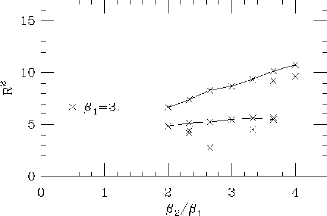
FIG. 4.: Mean-square radius of a single skyrmion, $\beta_{1}=3$. The upper curve connects the radii of stable configurations; other points are radii of metastable skyrmion configurations.

The multiple values of $R^{2}$ at a given value of $\beta_{2}$ reflect metastability. These metastable skyrmion configurations are accessible from different initial states, specified by different values of $r_{0}$ in Eq. (10). We have observed tunneling from metastable states to lower-energy states of larger radius that are apparently the global minima of the action. In all cases the lowest-energy states appear to be those of largest radius; these are shown connected by the upper curve in Fig. 4. The lower curve in the figure connects metastable states that were found to be mutually accessible by annealing. We have not explored the full set of metastable states for any given coupling; except for the annealing curve, the metastable states shown in Fig. 4 are effectively chosen at random by the initial conditions of the simulations.

In Fig. 5 we present a more extensive set of results, this time showing variation with $\beta_{1}$ as well as with $\beta_{2}$.

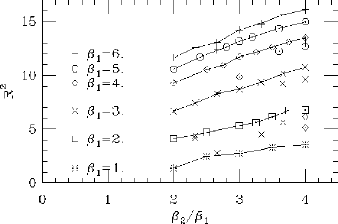
FIG. 5.: Mean-square radius of the topological density in the single-skyrmion sector

The curves connect data points for what we believe to be the equilibrium skyrmion configuration at each coupling. Points not lying on curves are metastable configurations of higher energy; again, we make no effort to show all such configurations at any coupling. We have not run across metastable configurations for $\beta_{1}\leq 2$.

The abscissa in Fig. 5 is the ratio $\beta_{2}/\beta_{1}$ that fixes the form of the action. The remaining overall coefficient $\beta_{1}$ then acts as an inverse temperature that governs the fluctuations. Regarding the 3d classical model as a Ginzburg-Landau theory for the fully quantized 4d theory, the lowering of $\beta_{1}$ can be interpreted as enhancing the thermal and quantum fluctuations in the latter. It is remarkable that heating the skyrmion by lowering $\beta_{1}$ causes it to shrink. We ascribe this surprising property to the many metastable, excited states that are smaller than the ground-state configuration and that become accessible as the temperature is raised. The absence of metastability at the smallest values of $\beta_{1}$ merely reflects the fact that the equilibrium skyrmion already averages over the various local minima.

VI Discussion

The qualitative conclusion of the preceding section must be taken with a large grain of salt. As mentioned above, we have no idea what the connection is between the couplings $\beta_{1}$ and $\beta_{2}$ of the 3d model on the one hand and the couplings and temperature of the 4d theory on the other. It is possible that raising the physical temperature of the latter will lead to simultaneous changes in $\beta_{1}$ and $\beta_{2}$ that cause the skyrmion to expand after all. In any case, the result is not quantitative and cannot be made quantitative until the dimensional reduction to the 3d theory is explored in detail. The metastable solutions, for that matter, might be artifacts of the specific lattice action we study that are absent in the true effective 3d theory.

Our study of the 3d model was motivated by its simplicity rather than by any fundamental obstacle to studying the full 4d theory at finite temperature. Numerical work on the 4d theory will merely require greater computer resources. In order to extract physics from lattice calculations, we will have to renormalize the theory by fixing the bare couplings $\beta_{1}$ and $\beta_{2}$, and the lattice spacing $a$, in terms of physical quantities such as the $\pi\pi$ scattering length and the skyrmion mass and radius. The temperature can be varied by changing the time extent $L_{t}$ of the lattice in the time direction, or by varying the lattice spacing by changing $\beta_{1}$ and $\beta_{2}$ along lines of constant physics. The 4d quantum theory will offer as well the possibility of projecting the skyrmion to definite spin and isospin. Finally, it will be imperative to study the sensitivity of any physical quantities to the choice of lattice action.

We collect in this appendix some practical details concerning the use of the Schläfli function (28) in calculating the topological density in lattice field configurations.

1 Small qrt’s

Defining

$$X\equiv\frac{\sin x\sin z-D}{\sin x\sin z+D},$$ (31)

the formula for the Schläfli function is

$$S(x,y,z)=\sum_{m=1}^{\infty}(-X)^{m}\frac{\cos 2mx-\cos 2my+\cos 2mz-1}{m^{2}}-x^{2}+y^{2}-z^{2}.$$ (32)

The sum converges absolutely when $|X|\leq 1$; since $D>0$, this means $\sin x\sin z>0$, which includes the entire domain (26) considered by Coxeter. In the Euclidean limit, where the qrt is small, we have $D\to 0$ and hence $X\to 1$. Then the sum in Eq. (32) becomes the Fourier series for $x^{2}-y^{2}+z^{2}$, and thus $S=0$ in this limit as expected.

The region of small $D$ is where the series converges most slowly. We can avoid evaluating Eq. (32) in this region as follows [7]. The vertices of a small tetrahedron in the 3-sphere are marked by 4-vectors $\mathchoice{{\hbox{\boldmath$\displaystyle\sigma$}}}{{\hbox{\boldmath$\textstyle\sigma$}}}{{\hbox{\boldmath$\scriptstyle\sigma$}}}{{\hbox{\boldmath$\scriptscriptstyle\sigma$}}}^{(i)}$ that are nearly equal. These 4-vectors are edges of a spindly 4-pyramid with its apex at the center of the 4-ball bounded by the 3-sphere, the volume of which is

$$V_{4}=\frac{1}{24}\epsilon_{\mu\nu\rho\sigma}\sigma^{(1)}_{\mu}\sigma^{(2)}_{\nu}\sigma^{(3)}_{\rho}\sigma^{(4)}_{\sigma}.$$ (33)

The ratio of $V_{4}$ to the total volume $\pi^{2}/2$ of the 4-ball is approximately the ratio of the 3-volume $V$ of the tetrahedron to the total volume $2\pi^{2}$ of the 3-sphere, so

$$V\approx 4V_{4}.$$ (34)

We calculate $V_{4}$ for every tetrahedron obtained for each lattice cube (see Fig. 1). If it is small, we use Eq. (34) in lieu of cutting it into qrt’s. We also calculate $V_{4}$ for each qrt in turn, and if it small we use Eq. (34) in lieu of evaluating the Schläfli function. Evaluation of $V_{4}$ also gives an easy way to keep track of the sign of a qrt’s volume, which is needed since $S(x,y,z)$ is defined always to be positive.

2 Large tetrahedra

Another problem region for the Schläfli function arises when $\alpha\to\frac{\pi}{2}$ or $\gamma\to\frac{\pi}{2}$, giving $X\to-1$ and slow convergence. In the limit $X=-1$, we have

$$S(x,y,z)=\pi(-x+y-z)=\pi\left(\alpha+\beta+\gamma-\pi\right),$$ (35)

a useful approximate formula in this regime.

As we have noted, Coxeter’s formula can only be used in the domain (26). One can easily devise larger qrt’s, however, and large qrt’s arise regularly in calculating the topological density. We attack this problem by cutting such large qrt’s into smaller tetrahedra. If either $\alpha$ or $\gamma$ is larger than $\frac{\pi}{2}$, but not both, we determine the largest of $\alpha,\beta,\gamma$ and draw a plane through its edge and the bisection point of the opposite edge (see Fig. 6).

FIG. 6.: Cutting a qrt in the event that $\alpha$ is too large.

This creates two new, smaller tetrahedra. If both $\alpha$ and $\gamma$ are larger than $\frac{\pi}{2}$, we cut the tetrahedron by connecting all its edge centers; this gives four tetrahedra at the original vertices, plus a central octahedron. The octahedron can then be cut into four tetrahedra around any line connecting opposite vertices, of which we choose the shortest.

Having cut the original qrt into two or eight pieces, we apply the algorithm (cut into qrt’s and apply the Schläfli function) to each piece. Of course, any qrt that results might still be too large for Coxeter’s formula. We then apply the cutting algorithm recursively. We have found that ten levels of recursion might be necessary for particularly rough lattice configurations.

The amount of recursion can be cut down dramatically by optimizing the operation of cutting the original tetrahedron into qrt’s. There are four ways to choose the vertex A in Fig. 3. For each choice of A, we determine the longest edge of the generated qrt’s, measured by the largest pairwise angle among the 4-vectors $\mathchoice{{\hbox{\boldmath$\displaystyle\sigma$}}}{{\hbox{\boldmath$\textstyle\sigma$}}}{{\hbox{\boldmath$\scriptstyle\sigma$}}}{{\hbox{\boldmath$\scriptscriptstyle\sigma$}}}^{(i)}$ of each qrt. This maximal edge is a measure of the size of the qrt’s generated by the cutting process. We choose A in order to minimize the maximal edge.

REFERENCES

- [1] T. H. Skyrme, Proc. Roy. Soc. Lond. A260, 127 (1961).
- [2] E. Witten, Nucl. Phys. B223, 433 (1983).
- [3] G. S. Adkins, C. R. Nappi and E. Witten, Nucl. Phys. B228, 552 (1983).
- [4] A. P. Balachandran, in High Energy Physics 1985, ed. by M. J. Bowick and F. Gürsey (World Scientific, Singapore, 1985).
- [5] I. Zahed and G. E. Brown, Phys. Rept. 142, 1 (1986).
- [6] R. Saly, Phys. Rev. D 31, 2652 (1985).
- [7] C. DeTar, Phys. Rev. D 42, 224 (1990).
- [8] S. Weinberg, Physica A96, 327 (1979).
- [9] J. Gasser and H. Leutwyler, Annals Phys. 158, 142 (1984); Nucl. Phys. B250, 465 (1985).
- [10] J. Bijnens, G. Ecker and J. Gasser, hep-ph/9411232.
- [11] N. Dorey, M. P. Mattis and J. Hughes, Phys. Rev. D 49, 3598 (1994) [hep-th/9309018]; 50, 5816 (1994) [hep-ph/9404274].
- [12] H. S. M. Coxeter, Q. J. Math. (Oxford Ser.) 6, 13 (1935), reprinted in H. S. M. Coxeter, Twelve geometric essays (Southern Illinois U. P., Carbondale, Ill., 1968), p. 4. The latter has been reprinted under the title The Beauty of Geometry (Dover, Mineola, N.Y., 1999). See also H. S. M. Coxeter, Regular Polytopes, 2nd ed. (Macmillan, New York, 1963; reprinted by Dover, New York, 1973).
- [13] L. Schläfli, Q. J. Pure App. Math. 2, 269 (1858); 3, 54 (1860); 3, 97 (1860); Theorie der vielfachen Kontinuität, Denkschr. Schweiz. Naturforsch. Ges. 38, 1 (1901).
- [14] R. S. Ward, Lett. Math. Phys. 35, 385 (1995) [hep-th/9502048].
- [15] S. L. Adler and T. Piran, Rev. Mod. Phys. 56, 1 (1984).
- [16] D. M. Y. Sommerville, Proc. R. Soc. (London) A115, 103 (1927); An Introduction to the Geometry of n Dimensions (Methuen, London, 1929; reprinted by Dover, New York, 1958).
- [17] H. W. Richmond, Q. J. Pure App. Math. 34, 175 (1903).