Operator Product Expansion on the Lattice: a Numerical Test in the Two-Dimensional Non-Linear -Model
Abstract
We consider the short-distance behaviour of the product of the Noether currents in the lattice nonlinear -model. We compare the numerical results with the predictions of the operator product expansion, using one-loop perturbative renormalization-group improved Wilson coefficients. We find that, even on quite small lattices (), the perturbative operator product expansion describes that data with an error of 5-10% in a large window . We present a detailed discussion of the possible systematic errors.
1 Introduction
The lattice regularization is nowadays the best theoretical tool for the study of nonperturbative phenomena in field theories. It has been extensively applied to QCD, providing quantitative predictions for many non-perturbative quantities, and it has also been extensively used in the study of strong-interaction effects in weak processes. One of the basic problems one has to deal with in these investigations is the determination of renormalized operators. Referring to the simple case of a purely multiplicative renormalization, given a “bare” operator on a lattice of size , we want to find a renormalized operator related to by
| (1.1) |
In Eq. (1.1) we have emphasized the dependence of the renormalization constant upon the various scales of the problem: the lattice spacing , which encodes the dependence on the bare coupling constant , the renormalization scale , the physical scale (the so called “-parameter”), which breaks the scale invariance of the continuum theory, and the size of the lattice . The constant should be defined so that has a finite continuum limit. In other words, the limit (i.e. ), , at fixed ,
| (1.2) |
should be finite.111Eq. (1.2) is a symbolic notation. Explicitly it indicates that correlations of with renormalized fields have a finite continuum limit. It is important to notice that the two limits in Eq. (1.2) do not commute, the infinite-volume limit should be taken before the continuum extrapolation . The renormalization constant admits a smooth infinite-volume limit at fixed . The behaviour in the continuum limit is instead singular and it is predicted by the renormalization group (RG). An exception is represented by operators that are conserved, at least in the continuum limit. In this case, the renormalization constant has a smooth continuum limit and does not depend on the scale . Examples of such operators are the vector and axial flavour currents in QCD and the energy-momentum tensor. In this case, the renormalization constants can be found by requiring the validity of the Ward identities related to the conservation of the operator [1, 2, 3, 4].
More difficult is the computation of the renormalization constants when the operator is not conserved. In this case, one can use lattice perturbation theory. However, these calculations are very tedious and long and one is usually restricted to one-loop order. A general non-perturbative strategy has been proposed in Ref. [5] and extensively studied since then, see, for instance, Ref. [6]. It provides a direct method for the computation of the renormalization constant appearing in (1.1). The main difficulty is the continuum limit, Eq. (1.2), which requires to keep under control the lattice artifacts and the finite-size effects. In practice, the method works only if there exists a window
| (1.3) |
in which lattice artifacts and finite-size effects are sufficiently small. Conditions (1.3) are not enough since we also want to relate to renormalized operators defined in continuum, say , perturbation theory. Since we want to apply continuum perturbation theory, we need additionally
| (1.4) |
A different renormalization method exploits finite-size effects and it is based on the observation due to Symanzik [7] that renormalizability is not spoiled when a field theory is considered on a finite space-time manifold. We can define a renormalization scheme by using the lattice size (instead of the external momentum employed in the preceding scheme) as the relevant energy scale. Finite-size scaling schemes have been much studied in the last years [8, 9, 10, 11, 12, 13, 14]. They have been successfully applied to the computation of the -parameter, of the light-quark masses and of the renormalized axial current in quenched QCD. With respect to the previous method, there is the advantage that the requirements (1.3) reduce to the weaker ones
| (1.5) |
Recently, a new method for the determination of renormalized composite operators in asymptotically free theories has been proposed in [15, 16, 17, 18]. It is based on the Operator Product Expansion (OPE), which has been postulated for the first time by Wilson [19] thirty years ago. It has been proved in perturbation theory by Zimmermann [20], and it is widely thought to hold beyond perturbation theory. This new procedure shares many features of the infinite-volume schemes and in fact it is defined in infinite volume, but it has the advantage of being more direct. It provides the matrix elements directly in continuum schemes and therefore, it could be the method of choice in those cases in which the renormalized operators are obtained as combinations of many different lattice operators. Moreover, it avoids the evaluation of products of local operators at coincident points. This fact reduces lattice artifacts and allows a simpler implementation of operator improvement.
We proceed now to describe the general context to which this method applies. Let us consider, for instance, the following simple example of OPE:
| (1.6) |
where the dots indicate terms of higher order in , corresponding to operators of higher canonical dimension. Let us suppose that we know how to define the renormalized operators and nonperturbatively. For instance, this is the case if they are conserved currents: If the lattice does not break the corresponding symmetry, one can choose a discretization in which they are exactly conserved and therefore, do not renormalize.
Let us suppose that we are interested in computing some hadronic matrix element of which we shall denote by . The proposed procedure works as follows:
-
1.
The Wilson coefficient is calculated using RG-improved perturbation theory. Any renormalization scheme can be used in this step, but we will usually consider the scheme. Moreover, to avoid spurious scale dependences, we consider RG-invariant (RGI) Wilson coefficients and correspondingly RGI operators. We indicate by the resulting -loop approximation for the Wilson coefficient.
-
2.
The matrix element is computed in a numerical simulation for a properly chosen range of , say for . This step gives a function .
-
3.
Finally, is fitted using the form and keeping as the parameter of the fit.
The result will be a function of , , and of the considered range . The physically interesting quantity222One could also consider the OPE in a finite physical volume. In this case, one would take the infinite-volume limit and the continuum limit together, keeping the physical volume fixed. is then
| (1.7) |
Note that the limits cannot be interchanged. First, we should consider the infinite-volume limit, then the scaling (continuum) limit at fixed , and , and finally take the short-distance limit. The outcome of this step,333 Notice the close resemblance with the so-called “point-splitting” renormalization procedure proposed a long time ago by Dirac [21]. , is identified with the matrix element we are looking for, , renormalized in the same scheme in which we computed the Wilson coefficient .
In practice, one works at finite values of and . However, one may still hope that there exists a window of values of such that , so that is small enough to allow the application of perturbative OPE and still large enough to make lattice artifacts small. The volume must of course be large enough to avoid size effects. Notice that the condition replaces here the condition , being the momentum at which renormalization is performed, present in standard infinite-volume schemes. In this respect the OPE method is not different from the standard renormalization methods.
The OPE has already been used in lattice simulations. For instance, in Refs. [22, 23, 24, 25, 26] the authors consider quark and gluon two-point functions in QCD. Their aim is to compute the (chiral and gluon) condensates. They use an “OPE-inspired” phenomenological fitting form, considering the condensates as fitting parameters. In all these and similar studies vacuum expectation values of short-distance products are considered. The possibility of varying the external states, investigated in this paper, provides a stronger check of the OPE and could be a fruitful resource.
An approach which allows to bypass the perturbative computation of the Wilson coefficient (with the related limitations) has been proposed in Refs. [27, 28]. The idea has been tentatively applied to the evaluation of the momenta of the nucleon structure functions. This method allows to study the structure functions at energy scales .
In this paper we perform a feasibility study of the procedure outlined above in the two-dimensional nonlinear -model. This model is quite interesting since it shares with QCD the property of being asymptotically free with a nonperturbatively generated mass gap [29, 30, 31]. It has also been extensively studied in perturbation theory, both in the continuum [32, 33, 34] and on the lattice [35, 36, 37, 38, 39, 40, 41, 42]. Extensive simulations have been done to check whether the theory shows the correct behaviour predicted by the perturbative RG [43, 44, 45, 46, 47, 38, 48] and to test the exact predictions for the mass gap obtained using the thermodynamic Bethe ansatz [49, 50]. Another advantage of this model is the availability of a very efficient algorithm [51, 52, 44], which shows no critical slowing down (for a general discussion see Ref. [53]). Therefore, we can work on very large lattices keeping the size effects completely under control.
We consider the OPE of products of Noether currents, a particularly simple case since the current is exactly conserved and therefore does not need any renormalization. We discuss in detail all possible sources of systematic errors, by considering several different cases.
The paper is organized as follows. In Sec. 2 we define the model and the basic notations, and in Sec. 3 we give the OPE for the product of the Noether currents that will be studied numerically. Sec. 4 presents a detailed discussion of our numerical results. Our conclusions are presented in Sec. 5. In App. A and B we give our perturbative results, while in App. C we critically discuss different methods for the determination of the running coupling constant.
2 The lattice model
In this paper we consider the nearest-neighbor lattice nonlinear -model in two dimensions. The fields are unit-length spins and the action is given by
| (2.1) |
where , and is the bare lattice coupling constant (often one introduces ). The partition function is given by
| (2.2) |
As usual, we introduce the lattice -parameter
| (2.3) | |||||
where is the lattice -function which can be expanded as
| (2.4) |
The coefficient are known up to four loops, i.e. for , see [35, 37, 41]. The first two coefficients are universal, and therefore, we have not added the superscript.
The mass gap of the model is related to the -parameter by
| (2.5) |
The constant is a nonperturbative quantity, and for generic models, it is usually unknown. For the nonlinear -model, an explicit expression has been obtained using the thermodynamic Bethe ansatz [49, 50]. Explicitly
| (2.6) |
In this paper we will consider the OPE of products of the Noether current, which is defined by
| (2.7) |
Because of the invariance of the theory, this current satisfies the Ward identity
| (2.8) |
where is a generic operator and . Since (2.8) holds exactly on the lattice, does not need to be renormalized.
A second operator we will be interested in is the energy-momentum tensor. In the continuum it is given by
| (2.9) |
The energy-momentum tensor is the Noether current of the translations, and therefore it is exactly conserved. On the lattice translation invariance is lost, and thus, there is no lattice operator whose naive continuum limit corresponds to (2.9) and that is exactly conserved. However, as shown in Ref. [56], it is possible to define an operator which is conserved in the continuum limit.444 The general ideas have been presented in [3], following closely the method used in [1] for the definition of the axial current. Explicitly one defines
| (2.10) |
where , is the naive lattice energy-momentum tensor,
| (2.11) |
and , , are renormalization constants. In Eq. (2.10) we have not considered terms that are not invariant and that vanish because of the equations of motion.555Similar terms appear also in QCD. Indeed, in this case, one should also consider, beside gauge-invariant operators, operators which are BRS variations and operators that are proportional to the equations of motion, see [4]. We have also discarded the contribution proportional to the identity operator (diverging as ), since it does not contribute to connected correlation functions. The renormalization constants have been computed to one-loop order in [56]. We have found a small error in one of the expressions. The correct results are reported in App. A.2.
3 OPE for the Noether currents
In this Section we report the general form of the OPE for the products of the currents. The coefficients are computed in perturbation theory, the explicit expressions to one-loop order being reported in App. B. As is well known, a perturbative expansion cannot be defined directly for the model (2.1) because of infrared singularities. A standard way out consists in adding a magnetic field that breaks the invariance of the theory and plays the role of infrared regulator. One considers therefore
| (3.1) |
A perturbative expansion is obtained setting , and expanding in powers of . When the integration measure is kept into account, the total action reads:
| (3.2) |
The calculation of the OPE is fairly standard and we report below the results in the continuum scheme and on the lattice for the cases that will be studied numerically.
3.1 The continuum scheme.
We begin by considering the OPE of the scalar product of two currents. The general form of the OPE is dictated by and rotational invariance and by power counting. The result can be written as follows:
| (3.3) | |||||
where and are functions of , of the coupling , and of the renormalization scale . Explicit one-loop expressions are reported in App. B.1. With we indicate the renormalized operator, while is the energy-momentum tensor (2.9). Notice the appearance of the operator ,
| (3.4) |
where the subscript indicates bare quantities. This operator is not invariant and its presence is due to the breaking of the invariance by the magnetic term. However, using the equations of motion, can be rewritten as
| (3.5) |
Therefore, on-shell and in the limit , we recover an -invariant expansion. Explicitly:
| (3.6) | |||||
with
| (3.7) |
The Wilson coefficients satisfy the following RG equations:
| (3.8) | |||||
| (3.9) | |||||
| (3.10) |
where is the -function.
We also consider the OPE of the antisymmetric product of the currents. Neglecting terms of order , we have666 Note that one could also add a contribution proportional to . However, in two dimensions, , and thus this term is equivalent to that proportional to .
| (3.11) |
The coefficients and satisfy the RG equations:
| (3.12) |
3.2 Lattice
On the lattice one can write expansions completely analogous to those holding in the continuum. The only difference is the appearance of terms that are cubic but not rotationally invariant. For the scalar product of two currents we obtain
| (3.13) | |||||
Here is the lattice energy-momentum tensor defined in Eq. (2.11), and is the lattice analogue of the quantity defined in Eq. (3.4),
| (3.14) |
where . Note the last term in Eq. (3.14) that is not present in the continuum and which is due to the measure term in the functional integral. Using the lattice equations of motion, one can show that
| (3.15) |
Therefore, on-shell and in the limit , it is possible to get rid of the terms proportional to as we did before.
In the antisymmetric sector we can write
| (3.16) |
3.3 RG-improved Wilson coefficients
We want now to resum the Wilson coefficients using the RG. We assume that the Wilson coefficient satisfies the equation
| (3.17) |
where is the (scheme-dependent) -function and is related to the anomalous dimensions of the operators appearing in the OPE. Such an equation is not valid in general, since for generic operators is a matrix. However, in the cases we are interested in, cf. Sec. 3.1 and 3.2, we can consider as a scalar function of and thus apply Eq. (3.17).
The general solution of Eq. (3.17) is easily found. If we define a running coupling by
| (3.18) |
then
| (3.19) |
It is useful to rewrite this equation as
| (3.20) |
where
| (3.21) |
where we have expanded . The factor may be included in the definition of the operator, introducing
| (3.22) |
where is the anomalous dimension of . The new operator is called RG invariant, in the sense that it satisfies a RG equation of the form
| (3.23) |
where is the -point irreducible correlation function with one insertion of . In other words, with this new definition, we have eliminated the running due to the anomalous dimension of the operator. Note, however, that, in spite of the name, this definition is not scheme independent.
Eq. (3.18) can be written as
| (3.24) |
which shows that is a function of only, i.e. . Moreover, defining , we can expand in inverse powers of . Explicitly, we obtain
| (3.25) |
Since the function is known to four-loop order, both on the lattice and in the scheme, two additional terms can be trivially added to this expansion, neglecting terms of order .
Finally, we wish to point out a further interpretation of . Consider for instance the scheme and correspondingly the coupling which is a function of , where is the mass gap. Then, it is easy to show using the RG equations that . In other words, is nothing but the coupling constant computed at the scale .
Finally, notice that the results presented in this Section can be applied to any renormalization scheme. In the following, we will use them to resum continuum predictions as well as lattice perturbative expressions.
4 Numerical results
In this Section we present our numerical computations meant to verify the feasibility of the nonperturbative renormalization method presented in the Introduction.
We consider matrix elements of the product of two Noether currents between one-particle states. This case is particularly simple, because the currents are exactly conserved and the matrix elements of the operators that appear in the OPE expansion can be computed exactly in most of the cases.
The typical procedure we adopt is the following:
-
1.
We compute a matrix element measuring a suitable lattice correlation function.
-
2.
We compute the matrix element appearing in the OPE expansion either exactly (as is possible in most of the cases) or numerically by means of some different numerical nonperturbative technique.
-
3.
We divide by the OPE prediction .
The goal is to see if there is a window of values of in which the OPE works, i.e. the result of step 3 is 1 independently of . For the cases we will consider here, the OPE gives an accurate description (at the level of 5-10%) of correlation functions for distances (from now on we set ). This result is quite encouraging for future applications of this method.
4.1 The observables
We have simulated the -model with action (2.1) using a Swendsen-Wang cluster algorithm with Wolff embedding [51, 52, 43, 53]. We did not try to optimize the updating procedure: Most of the CPU time was employed in evaluating the relevant observables (four-point functions) on the spin configurations of the ensemble. In order to estimate the scaling corrections, we simulated three different lattices, of size , using in all cases periodic boundary conditions:
-
(A).
Lattice of size with .
-
(B).
Lattice of size with .
-
(C).
Lattice of size with .
The algorithm is extremely efficient—the dynamic critical exponent is approximately 0—and the autocorrelation time is very small. We performed a preliminary study in order to determine how many iterations are needed to obtain independent configurations. For this purpose we measured the normalized autocorrelation function
| (4.1) |
for different observables . Here is the number of Monte Carlo iterations, is the value of at the -th iteration, and the sample mean of . In Fig. 1 we report for the observable
| (4.2) |
where and . We have considered —a short-distance observable—and . As expected, local observables have a slower dynamics—this is due to the fact that the dynamics is nonlocal—than long-distance ones. In any case, for all observables the autocorrelation function shows a fast decay: indeed, for we have , while for we have . Moreover, is independent of the lattice used, confirming the fact that (as we shall report below, all lattices have the same ). Since the measurement of the observables is quite CPU-time consuming, we computed the relevant correlation functions only every 15 iterations, which should be enough to make the measurements independent. Nonetheless, most of the CPU time is employed in evaluating the observables on each spin configuration of the ensemble. We computed the product of two Noether currents for distances smaller than some fixed fraction of the correlation length: . If the physical size of the lattice is kept constant (as we did) we expect the CPU time to scale as . The CPU time per iteration turns out to be roughly independent of the particular product considered. As an example we give the CPU time per measurement for the simulation in which we compute the antisymmetric product of two currents between states with opposite momentum. For the three different lattices, on an SGI Origin2000, we have: , , .
We measure several different observables. First, we measure the two-point function (here and in the following the “temporal” direction is the first one, of extent )
| (4.3) |
We computed the correlation function on the lattices (B) and (C) for momenta and times separations ; on lattice (A) we considered the same set of momenta and time separations . The number of independent configurations we generated is: for lattice (A); for lattice (B); for lattice (C) and ; finally for lattice (C) and .
A check of our simulation is provided by the results of Ref. [57], who computed, among other things, the mass gap for lattices (A) and (B). For the exponential correlation length we obtain
| (4.4) |
for lattices (A), (B), (C) respectively. They are in good agreement with the results of Ref. [57]: they obtain and for the first two lattices. The three lattices we simulate have approximately the same physical size, , which is large enough to make finite-size effects much smaller than our statistical errors. This is confirmed by the analysis of Ref. [57].
In order to verify the OPE, we need the values of the matrix elements which appear in the r.h.s. of Eq. (1.6). Matrix elements of lattice operators can be computed from properly defined three-point correlation functions. If is a lattice operator, we define the correlation function
| (4.5) |
and the corresponding normalized correlation
| (4.6) |
The function has a finite limit for . In this work we will only need the matrix elements of the naive lattice energy-momentum tensor (2.11). For this reason, we have computed with . Such a correlation function has been computed on lattice (B), using configurations, for and , . For these observables is independent of , within the statistical errors, already at . The results obtained for are reported in Table 1. For , statistical errors are dominated by the error on the evaluation of . On the other hand, for , the statistical error of the numerator in Eq. (4.6) is roughly equal to that of the denominator. The reason is clear: since in the continuum limit is proportional to the identity operator, we are computing essentially (up to corrections) the same quantity in the numerator and in the denominator with approximately the same statistics. The reported errors on the ratios are obtained using the independent error formula. For smaller error bars could have been obtained by taking into account the statistical correlations between numerator and denominator.
We also measured for the same operators on lattice (B), using independent configurations, for with and . The normalized three-point function shows a plateau for when and for when . The results obtained for are reported in Tab. 2. In this case the statistical errors are dominated by the uncertainty on .
In this paper we study the OPE of the product of two currents. Therefore, we have computed the following correlation functions:
| (4.7) | |||||
| (4.8) |
where is the lattice Noether current defined in Eq. (2.7). Of course, we averaged over lattice translations.
In particular we have measured:
- a)
-
b)
using independent configurations on lattice (B).
- c)
-
d)
using independent configurations on lattice (B).
In all cases we consider , ; and on lattice (A), and on lattice (B), and and on lattice (C).
Using the four-point correlation function determined above, we constructed the normalized ratios
| (4.9) |
which have a finite limit for . We verified that is independent of in the range considered, and thus we have taken the estimate corresponding to the lowest considered value of as an estimate of .
In the paper we will usually consider averages over two-dimensional rotations, i.e., given a function , we consider
| (4.10) |
with and , integer.
4.2 One-particle states
In the conventional picture the lowest states of the model are one-particle states transforming as vectors. On a lattice of finite spatial extent , we normalize the states and the fields as follows:
| (4.11) | |||||
| (4.12) |
The function , which is the energy of the state , and the field renormalization can be determined from the large- behavior of the two-point function :
| (4.13) |
In the continuum (scaling) limit we have independent of and . In Table 3 we report our results for the three lattices. In order to evaluate and we determined effective values at time by solving the equations
| (4.14) | |||||
| (4.15) |
Then we looked for a plateau in the plot of and versus . Both functions become independent of for . The values reported in Table 3 correspond to one particular value of of order : respectively for lattice (A), (B), (C). For the two largest lattices there is evidence of scaling at the error-bar level. Instead, for lattice (A) there are tiny scaling violations, that are however so small (at most 1%) that we can neglect them in the following discussion.
One can also investigate asymptotic scaling, i.e. the dependence of and on . The dependence of can be determined from Eq. (2.5). There exists also an exact prediction for , including the nonperturbative constant [58, 59]. However, as is well known, lattice perturbation theory is not predictive at these values of the correlation length, and indeed, the perturbative four-loop predictions show large discrepancies compared to the numerical data. The agreement is instead quite good [47, 59] if one uses the improved coupling defined in Eq. (C.7).
4.3 Nonperturbative renormalization constant for the lattice energy-momentum tensor
In this Section we want to compute nonperturbatively the renormalization constant of the lattice energy-momentum tensor (2.10). In general, given an operator on the lattice we define its matrix element by
| (4.16) |
For the matrix elements can be obtained from the results given in Tables 1 and 2. The matrix elements of are dominated by the mixing with the identity operator and thus, in order to define the renormalized operator for , we should perform a nonperturbative subtraction of the large term, which is practically impossible.777In general we expect and . The quantity we are interested in is . However, from Table 1 we immediately realize that much smaller errors are required to really observe the momentum dependence of the matrix elements and thus to determine the constant . Therefore, we only compute the renormalized operator for , which amounts to determining the constant . This constant is obtained by requiring
| (4.17) |
In practice, we first compute an effective (momentum-dependent) renormalization constant
| (4.18) |
which, in the continuum limit, becomes independent of and converges to . Using the data of Table 1, on lattice (B), we obtain , , for , , respectively. Clearly the scaling corrections are small, and thus we can estimate on this lattice. This compares very well with the result of one-loop lattice perturbation theory given in Eq. (A.47), which yields , and with the result of “improved” (sometimes called “boosted”) perturbation theory in terms of the coupling , cf. Eq. (C.7), (the error is due to the error on ).
4.4 OPE for the scalar product of currents
In this Section we consider the product averaged over rotations. Using Eq. (3.3), we have in the continuum scheme
| (4.19) |
All other contributions vanish after the angular average. Using the results of App. B.1 we have at one loop in the scheme
| (4.20) |
where is the renormalization scale and Euler’s constant. We will not use this form of the OPE expansion, but instead the RG-improved Wilson coefficients. Thus, cf. Sec. 3.3, we write
| (4.21) |
where
| (4.22) |
and is the running coupling constant defined by888This equation should be intended as follows: in the right-hand side is assumed given, while for we intend its expression in terms of the -function, Eq. (C.2).
| (4.23) |
Using the perturbative expression (3.25), we can also rewrite (4.22) as
| (4.24) |
where .
We will also use the lattice Wilson coefficients defined in Sec. 3.2. Using the one-loop results of App. B.3 and the general expressions reported in Sec. 3.3, proceeding as before, we obtain the prediction
| (4.25) |
where, at one loop,
| (4.26) | |||||
| (4.27) |
and is the running coupling constant defined by
| (4.28) |
where is the lattice -parameter (2.3).
Finally we shall test perturbation theory in the “improved” expansion parameter defined in Eq. (C.7). The OPE becomes:
| (4.29) |
where
| (4.30) |
is the same as in Eq. (4.27), and is the running coupling constant defined by
| (4.31) |
where is the -parameter (C.9).
We have tested the validity of the OPE by considering matrix elements between one-particle states. The matrix elements of the product of the currents999 Since the currents are exactly conserved, both on the lattice and in the continuum, there is no need to make a distinction between lattice and -renormalized operators. can be determined in terms of , since
| (4.32) |
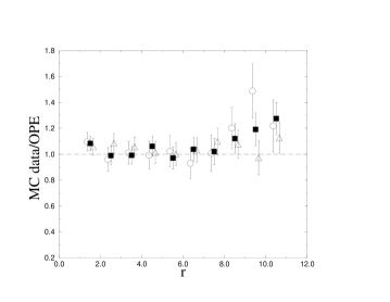
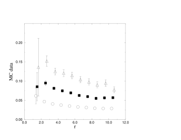
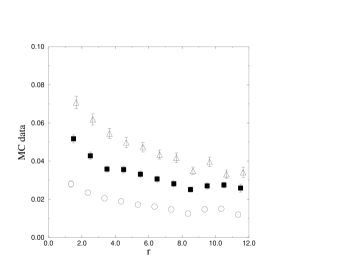
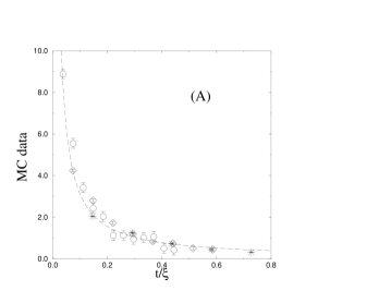
In Fig. 2 we report101010 On lattice (B) has only been measured in . The points with appearing in the figure correspond to “partial” angular averages, i.e. they have been obtained using Eq. (4.10) and restricting to . The same comment applies also to the subsequent figures. the angular average of for lattices (A) and (B): here , for the two lattices respectively. In Figs. 3, 4, and 5 we compare these numerical data with the predictions of perturbation theory.
In Fig. 3 we use continuum RG-improved perturbation theory in the scheme. In this case, the matrix element of the energy-momentum tensor is immediately computed: . Therefore, we consider the ratio
| (4.33) |
which should approach 1 in the short-distance limit. In Fig. 3 we present several determinations of that differ in the way in which the running coupling constant and the coupling are determined.
There are several different methods that can be used to compute the coupling and the strictly related . They are compared in detail in App. C. It turns out that the finite-size scaling method proposed by Lüscher [60, 61] and what we call “the RG-improved perturbative method” are essentially equivalent, see, e.g., Table 4 in App. C. Therefore, we can use either of them,111111In QCD the RG-improved perturbative method cannot be used since no exact prediction for the mass gap exists. In this case the finite-size scaling method would be the method of choice. Note that for large values of the scale also the improved-coupling method [62, 63], which can be generalized to QCD [64], works well, see App. C. obtaining completely equivalent results. In Fig. 3 we have used the finite-size scaling method to be consistent with what we would do in QCD. Elsewhere, we have used the RG improved perturbative method because of its simplicity.
The first step in the computation of is the determination of . This is obtained as follows: we fix , and using the finite-size scaling results reported in Table 4 in App. C, we compute . Then, using Eq. (C.4) we determine at -loops. Finally, is obtained either by solving Eq. (4.23), again using Eq. (C.4) for appearing in the right-hand side, or by using Eq. (3.25). As we discussed in Sec. 3.3, the final result should be independent of the chosen value of and therefore we can evaluate the systematic error on by considering different values of . If we fix , cf. first row of Table 4 in App. C, on lattice (B), we have , , respectively for , , , while if we fix , cf. 10th row of Table 4 in App. C, we have , , at the same distances. The dependence is tiny and, as expected, it increases for larger values of . In practice, it does not play any role, the main source of error being instead the truncation of the OPE coefficients. Notice that the independence on is obvious if we use the RG-improved perturbative method.
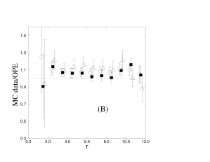
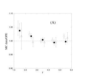
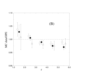
Let us now describe the various graphs appearing in Fig. 3. In graphs (A) and (B) we fix and then, using the results presented in Table 4, cf. first row, we obtain . We then compute using the four-loop expression (C.4) with . Finally, the Wilson coefficient is given by (4.24): in graph (A) we use the leading term only, while in graph (B) we include the next-to-leading one.
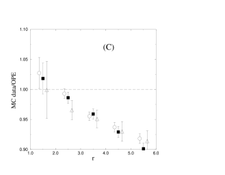
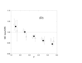
In graphs (C) and (D) we compute as in (A) and (B), choosing a different scale, , cf. row of Table 4. Then we compute by solving numerically Eq. (4.23) using the four-loop expression (C.4) with . Finally, the Wilson coefficient is obtained using Eq. (4.22). While in graph (C) we keep only the leading term , in graph (D) we use the complete expression.
Finally, graphs (E) and (F) are identical to graph (D) except that and are computed using the two-loop expression (C.4) with . The two graphs correspond to different choices of : (graph (E)) and (graph (F)).
Comparing the different graphs, we immediately see that the choice of scale and the order of perturbation theory used for (two loops or four loops) are not relevant with the present statistical errors. Much more important is the role of the Wilson coefficients. If one considers only the leading term (graphs (A) and (C)) there are indeed large discrepancies and in the present case one would obtain estimates of the matrix elements with an error of 50–100%. Inclusion of the next-to-leading term—this amounts to considering one-loop Wilson coefficients and two-loop anomalous dimensions—considerably improves the results, and now the discrepancy is of the order of the statistical errors, approximately 10%. For the practical application of the method, it is important to have criteria for estimating the error on the results. It is evident that the flatness of the ratio of the matrix element by the OPE prediction is not, in this case, a good criterion: The points in graph (A) show a plateau—and for a quite large set of values of —even if the result is wrong by a factor of two. However, this may just be a peculiarity of the case we consider, in which the -dependence of the data and of the OPE coefficients is very weak. On the other hand, the comparison of the results obtained using different methods for determining seems to provide reasonable estimates of the error bars. For instance, if only the leading term of the Wilson coefficients were available, we could have obtained a reasonable estimate of the error by comparing graphs (A) and (C).
In Fig. 4 we consider lattice RG-improved perturbation theory, computing
| (4.34) |
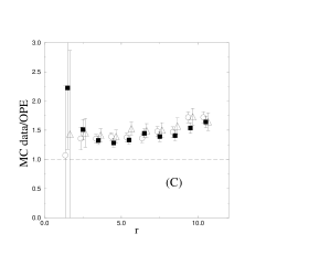
In graph (A) we use as an expansion parameter. We compute using the value of the mass gap and Eq. (2.5), with the nonperturbative constant (2.6). Then, we determine by solving numerically (4.28) and using for appearing in the left-hand side its truncated four-loop expression (2.3). Finally, we use Eq. (4.26) for the Wilson coefficient. The results are quite poor: there is a downward trend as a function of and the data are far too low. Naive lattice perturbation theory is unable to provide a good description of the numerical data.
The results improve significantly if we use the improved coupling : The estimates obtained using this coupling, graphs (B), (C), (D), are not very different from those obtained using continuum perturbation theory. Graph (B) has been obtained exactly as graph (A), except that in this case we used as an expansion parameter. The -parameter is defined in (C.9), in (C.10), and the relevant Wilson coefficient is given in Eq. (4.30). Graphs (C) and (D) are analogous to graph (B). The difference is in the determination of . We do not compute it nonperturbatively by using the mass gap but we determine it directly from the perturbative expression (C.9). In this case we use the perturbative expression truncated at four loops (C) and two loops (D).
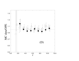
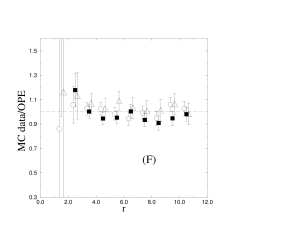
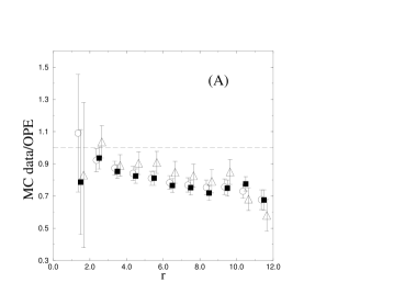
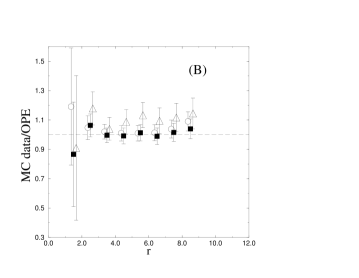
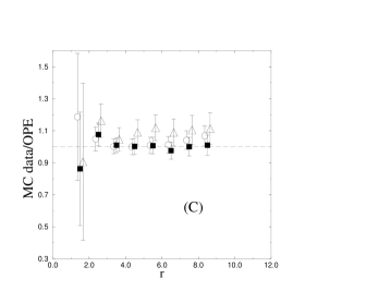
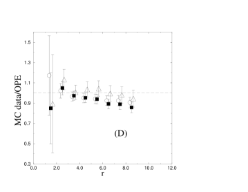
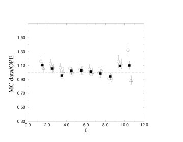
In Figs. 3, 4 we have checked the validity of the OPE on lattice (B). If one has in mind QCD applications this is quite a large lattice since . For this reason, we have tried to understand if the nice agreement we have found survives on a smaller lattice, by repeating the computation on lattice (A). The results are reported in Fig. 5. Graphs (A) and (B) should be compared with graph (D) of Fig. 3. In (A) we compute from Eq. (2.5), with the nonperturbative constant (2.6) and . Then, we compute solving numerically Eq. (4.23) using the four-loop expression (C.4) with . The Wilson coefficient is obtained from Eq. (4.22). In (B) we repeat the same calculation as in Fig. 3 graph (D) at the scale . In (C) and (D) we repeat the calculation of graph (B) using the two-loop and the three-loop -function for the determination of the coupling . In all graphs (B), (C), (D) we use the result .
Graphs (A) and (B) show a nice flat behaviour and for , the ratio is approximately 1 with 2–3% corrections (notice that the vertical scale in Figs. 3 and 5 is different): The OPE works nicely even on this small lattice. (A) and (B) differ in the method used in the determination of the coupling. As we explained in App. C and it appears clearly from the two graphs, the effect is very small. Graph (C)—and to a lesser extent graph (D)—shows instead significant deviations: Clearly, must be determined using four-loop perturbative expansions in order to reduce the systematic error to a few percent. Notice that such discrepancies are probably present also for lattice (B): however, in this case, the statistical errors on are large—approximately 5-6% (for and ) and 9% (for )—and thus they do not allow to observe this effect.
As a further check we considered matrix elements between states of different momentum. In Fig. 6 we report the angular average of for lattice (B). In Fig. 7 we compare the numerical data with the OPE prediction, by considering
| (4.35) |
where is defined in Eq. (2.10) and is computed in Sec. 4.3. In Fig. 7 we report for lattice (B). The Wilson coefficients are computed as in graph (A) of Fig. 5, using . The numerical data are again well described by the OPE prediction for a quite large set of values of .
4.5 OPE for the antisymmetric product of currents
In this Section we consider the antisymmetric product of two currents and compare our numerical results with the perturbative predictions. With respect to the previous case, we have here a better knowledge of the perturbative Wilson coefficients—some of them are known to two loops—and moreover we have an exact expression for the one-particle matrix elements of the current . Indeed, we have [65, 57]:
| (4.36) |
where , , , and, for ,
| (4.37) |
where the rapidity variable is defined by .
We first consider the product for and . The OPE of such a product can be determined from Eq. (3.11). Using the results of App. B.2, we have for ,
| (4.38) |
where, at two loops,
| (4.39) |
and is defined in Eq. (4.23). We also consider the angular average of the product of the currents for and . Using the results of App. B.1, we have for
| (4.40) |
Again, we have tested the validity of the OPE by considering matrix elements between one-particle states. The matrix elements of the product of the currents are obtained from
| (4.41) |
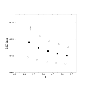
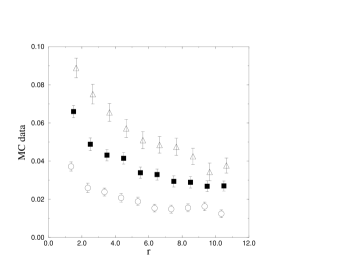
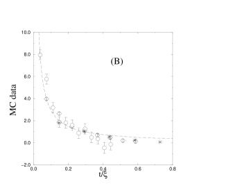
In Fig. 8 we show a plot of obtained on lattice (B) for and , and in Fig. 9 we show the angular average of on the same lattice and again for . Comparing these graphs with those for the scalar product of the currents, one sees that the matrix elements show here a larger variation with distance, and thus this should provide a stronger test of the validity of the OPE.
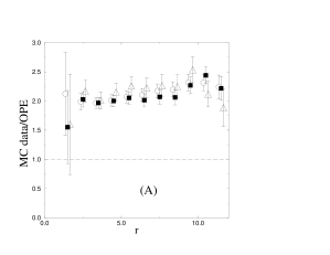
In Fig. 10 we compare the results for with the OPE perturbative predictions. Here, as always in this Section, we use the RG-improved perturbative method to compute , using the four-loop expression for the function. As we explained at length in the previous Section, no significant difference is observed if one uses the finite-size scaling method, or improved lattice perturbation theory.
In graphs (A) and (B) we show the combination
| (4.42) |
for two different values of . In the scaling limit is a function of and of . As it can be seen from the graphs our results show a very nice scaling: The data corresponding to the three different lattices clearly fall on a single curve. In the same graphs we also report the OPE prediction (4.38), i.e.
| (4.43) |
Note that , so that the corrections due to higher-order terms in the OPE expansion are of order . In graph (A) and (B) we use only the one-loop Wilson coefficient for . There is a good agreement between the OPE prediction and the numerical data: quite surprisingly the agreement extends up to 2 lattice spacings.
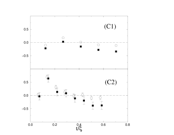
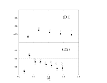
To better understand the discrepancies, in graphs (C) and (D) we report . In graphs (C1) and (C2) we use the one-loop Wilson coefficient, and in (D1) and (D2) the two-loop Wilson coefficient given in Eq. (4.39). The numerical data refer to lattice (A) for (C1) and (D1) and to lattice (B) for (C2) and (D2). There is clearly agreement, although here deviations are quantitatively somewhat large, since is strongly varying. Let us consider for instance the data obtained on lattice (B) for . If we evaluate the matrix element of the Noether current using the numerical estimate of with we obtain the result with a systematic error of respectively.
In Fig. 11 we compare the angular average of (cf. Fig. 9) with the OPE prediction, by defining
| (4.44) |
where is the OPE one-loop prediction (4.40). Here we use the form-factor prediction (4.36) for the matrix elements of the currents, but no significant difference would have been observed if the matrix elements of the currents had been determined numerically. Use of the form-factor prediction allows only a reduction of the statistical errors and thus gives the opportunity for a stronger check of the OPE. Again we observe a nice agreement and a very large window in which the data are well described by perturbative OPE. The systematic error is below the statistical one (which is approximately ) as soon as .
5 Conclusions
In this paper we have studied the OPE of the Noether currents in the two-dimensional -model. We have investigated in detail the possible problems that may arise in numerical applications. We can summarize the main results of this paper as follows:
-
1)
The relevant correlation (four-point) functions show a good scaling behaviour and can be determined on relatively coarse lattices (for instance on lattice (A)). Lattice corrections of order are negligible compared to statistical and systematic errors. Notice that we have used the standard action, so that we could have easily improved the scaling behaviour by using an improved action [66] and improved operators.
-
2)
The running coupling constant can be determined quite precisely. For instance, using the finite-size scaling method can be computed with an error of a few percent for the values of of interest. This error is practically negligible in our applications.
-
3)
The main source of error is in our case the perturbative truncation of the Wilson coefficients. If one uses one-loop RG-improved Wilson coefficients—this also requires the two-loop anomalous dimensions of the operators—one can compute the matrix elements with a precision of 5–10%. In practice, the precision of the results is limited by the statistical error, which is quite large: using independent configurations, we obtain results with a statistical uncertainty of 10%, so that improving the expressions for the OPE coefficients at two loops appears of little interest.
In conclusion the method works nicely for the cases we consider. In all cases, we observe a large window in which the numerical data are well described by one-loop OPE.
Acknowledgements
We thank Peter Weisz for useful correspondence, Guido Martinelli, Roberto Petronzio, Giancarlo Rossi, and Massimo Testa for suggestions and discussions.
Appendix A Renormalization of composite operators
A.1 Continuum scheme
In this Appendix we consider the nonlinear -model in dimensions. In terms of bare fields, the action is written as
| (A.1) |
In order to perform a perturbative expansion, the -vector field is parametrized as
| (A.2) |
The theory is renormalized by introducing the renormalized quantities
| (A.3) | |||||
| (A.4) | |||||
| (A.5) | |||||
| (A.6) |
where . Such a factor is introduced to implement naturally the prescription. The renormalization constants defined above are known to four-loop order in perturbation theory [67, 34, 68]. Here, we only need their one-loop expression:
| (A.7) |
The -function and the anomalous dimension of the field are obtained from the renormalization constants:
| (A.8) |
We also consider the renormalization of composite operators. In general, a renormalized composite operator can be written as
| (A.9) |
where the ’s are unrenormalized composite operators, that is products of the renormalized fields ’s, ’s and of their derivatives. Which operators appear in the r.h.s. of Eq. (A.9)? The naive answer is: all operators that transform under as and that satisfy . This answer is wrong because of the magnetic term in Eq. (A.1) that breaks explicitly the symmetry.121212 A similar problem is encountered in nonabelian gauge theories. In order to renormalize gauge-invariant operators, gauge noninvariant quantities must be considered. The correct answer has been given in [32, 69]. If we define the noninvariant operator
| (A.10) |
then we must also include all products of the type where has the correct transformation properties and satisfies . Note that can be rewritten as
| (A.11) |
so that, on-shell and in the limit , we recover an covariant mixing matrix. In other words, matrix elements between physical states have the correct transformation properties.
Finally, we note that, if the scheme is adopted, the renormalization constants are dimensionless so that the operators appearing in the r.h.s. of Eq. (A.9) satisfy .
In the following we report the renormalization constants for a few cases of interest.
A.1.1 invariant operators of dimension 2
We consider invariant operators of dimension 2. There are two such operators, and . For the renormalization we must also consider the operator defined in Eq. (A.10). They renormalize as follows:131313We adopt the following convention in reporting the renormalization constants. Given a basis of operators of dimension and isospin , their renormalization constants are defined by .
| (A.12) | |||||
| (A.13) | |||||
| (A.14) |
A particular combination of these operators is the energy-momentum tensor
| (A.15) |
For this particular set of operators, the renormalization constants can be directly related to and . Indeed, one first observes that is conserved. Therefore, it is finite when it is expressed in terms of bare fields. It follows:
| (A.16) |
Then, one notices that differentiation of the action (A.1) with respect to (and keeping , and constant) gives a finite operator, which is a combination of and . For this combination reduces to . Therefore, it can be identified with . The renormalization constants immediately follow:
| (A.17) | |||||
| (A.18) |
A second relation is obtained by using the fact that the equations of motion do not need any renormalization. It follows that the combination
| (A.19) |
is finite. Combining this result with what we obtained above, we conclude that
| (A.20) | |||||
| (A.21) |
The remaining renormalization constants can be obtained by using Eqs. (A.12-A.15):
| (A.22) | |||||
| (A.23) |
Note that Eq. (A.11) holds also for the renormalized operators. Indeed, using the expressions of the renormalization constants reported above, we can show that
| (A.24) |
In the limit and on-shell, Eq. (A.24) allows us to express matrix elements of the noninvariant operator in terms of those of the invariant operator .
A.1.2 Antisymmetric operators in two indices
We shall now consider operators that are antisymmetric tensors with two indices. Obviously, there is no such operator of dimension zero. The only antisymmetric operator of dimension is the Noether current corresponding to the symmetry:
| (A.28) |
Conservation of implies
| (A.29) |
There are three operators of dimension with the same symmetry. All of them can be expressed in terms of . Therefore, they renormalize as the current itself.
A.2 Lattice
We now consider the lattice action (3.1). If one neglects lattice artifacts of order , lattice correlation functions of and fields differ by a finite renormalization from those computed in any other scheme. Here we want to relate lattice correlations to the corresponding continuum ones computed in the scheme. The finite renormalization is given by
| (A.30) | |||||
| (A.31) | |||||
| (A.32) |
where the lattice fields appear in the left-hand side, the renormalized continuum fields in the right-hand side. The renormalization constants and have been computed to three-loop order in perturbation theory [37, 41]. We shall only need the one-loop result:
| (A.33) |
Analogously, we can relate -renormalized composite operators to the lattice corresponding ones. As in the continuum, besides invariant operators, we must also consider operators involving , cf. Eq. (3.14). However, also on the lattice, invariance is recovered when considering matrix elements between on-shell states. A second complication in the lattice approach is the loss of Lorentz invariance: as a consequence, additional operators that are only cubic invariant must be considered. Below we report the renormalization constants for a few cases of interest.
A.2.1 -invariant operators of dimension 2
On the lattice we have:141414In the following equations we have not reported an additional contribution proportional to , where 1 is the identity operator. This term does not contribute to connected correlation functions, and for this reason, we have not written it explicitly.
| (A.34) | |||||
| (A.35) | |||||
| (A.36) | |||||
| (A.37) |
Note the presence of an additional operator, which is cubic but not invariant. At one loop we obtain:151515 Some of the renormalization constants given below have been computed in Ref. [56]. We report them here to correct a few misprints.
| (A.38) | |||||
| (A.39) | |||||
| (A.40) | |||||
| (A.41) | |||||
| (A.42) | |||||
| (A.43) | |||||
| (A.44) | |||||
| (A.45) |
and . Finally, for the energy-momentum tensor, we have
| (A.46) | |||||
with
| (A.47) | |||||
| (A.48) | |||||
| (A.49) | |||||
| (A.50) |
Note that, since is conserved,
| (A.51) |
Finally, notice that we can eliminate using the lattice equations of motion
| (A.52) |
However, is different from appearing in all previous formulae. The two operators are related by a finite renormalization:
| (A.53) |
At one loop
| (A.54) |
Then, considering only connected correlation functions, on-shell and for , we have
| (A.55) |
Using this relation, we can compute appearing in Eq. (2.10). Explicitly
| (A.56) |
A.2.2 Antisymmetric operators in two indices
Let us consider operators which are antisymmetric tensor with two indices. As we discussed in the continuum case, there is only one relevant operator of dimension 1, the current. Since the symmetry is preserved on the lattice, there is a lattice discretization, given in Eq. (2.7), that is exactly conserved. It follows that
| (A.57) |
i.e. .
As in the continuum there are three operators of dimension 2. If on the lattice we express them in terms of , then also these operators do not need any renormalization.
Appendix B OPE for Noether currents
In this Appendix we report the explicit one-loop expressions of the OPE coefficients reported in Sec. 3.
B.1 Continuum
B.2 Constraints on the OPE coefficients
In this Section we want to derive the constraints due to the current conservation on the coefficients of the OPE. First, we need the Ward identity related to the invariance in the presence of a magnetic term . A simple calculation gives:
| (B.15) |
Then we need the OPE of . The leading term for has the form
| (B.16) |
Using Eq. (B.15) and noticing that for , we have . Thus, is a function of only. But the Wilson coefficient satisfies the RG equation
| (B.17) |
Thus, if it is independent of , and therefore of , it is also independent of . A simple calculation at tree level gives then
| (B.18) |
The same result has been obtained in [70] using the canonical formalism.
We now consider the OPE of the scalar product of currents. Using the Ward identity (B.15) and Eq. (B.18) we have for
| (B.19) |
where we have discarded contact terms. Then, using Eq. (A.24) and discarding again contact terms, we obtain for
| (B.20) |
This equation implies the following relations on the Wilson coefficients:
| (B.21) | |||
| (B.22) | |||
| (B.23) | |||
| (B.24) | |||
| (B.25) |
In the derivation we used Eq. (A.27) for the trace of the energy-momentum tensor.
Now let us consider the antisymmetric case. Using the Ward identity (B.15) and Eq. (B.18), we obtain for
| (B.26) |
Again, contact terms have been discarded in the derivation. Using this relation, we obtain the following constraints on the Wilson coefficients161616 Equations (B.27)–(B.31) have been derived in Ref. [70]. Eq. (B.32) is due to the matching of the terms proportional to . It is also a simple consequence of Eqs. (B.28) and (B.30) and of the RG equations.
| (B.27) | |||
| (B.28) | |||
| (B.29) | |||
| (B.30) | |||
| (B.31) | |||
| (B.32) |
Using Eqs. (B.27) and (B.28) we obtain immediately
| (B.33) |
which implies that this combination is and independent. By making use of the RG equations (3.12) one proves that this combination is determined uniquely by its one-loop value. Then, using the results of the previous Section, we obtain:
| (B.34) |
Thus, using (B.34) and (B.28), and are uniquely determined by . Moreover, using Eqs. (B.34) and (B.32) one immediately verifies that Eqs. (B.30) and (B.31) are equivalent to Eq. (B.28).
Finally, consider (B.29). We will now show that this equation provides the two-loop estimate of . Indeed, since
| (B.35) |
and , cf. previous Section, we have
| (B.36) |
where , and , are constants that are not fixed by the RG equation. Plugging this expression into (B.29), we obtain
| (B.37) |
Of course, the result at order agrees with the expression reported in Sec. B.1. Correspondingly we obtain
| (B.38) | |||||
| (B.39) | |||||
| (B.40) |
Let us finally mention that in Ref. [70] it was argued that the functions are one-loop exact, in the sense that there are no corrections of order , . As we have shown above and it has also been recognized by the author,171717In Ref. [71] it was also shown that, even though the expressions for the Wilson coefficients were incorrect, one could still modify the argument so that the main result (existence of a conserved charge) of Ref. [70] remains true. this is inconsistent with the RG equations.
B.3 Lattice
Appendix C Evaluation of the running coupling constant
The determination of the running coupling constant is a key ingredient in the application of RG-improved perturbation theory to any asymptotically free theory. If we use the lattice OPE, the coupling is the bare , one of the input parameters of our numerical calculations. However, perturbation theory in is poorly behaved, so that one expects a poor agreement with the numerical data. It is known that it is much more convenient to use perturbative expansions in the scheme. Perturbative coefficients are smaller, so that truncations in the number of loops give smaller systematic errors. For these reasons, it is important to relate the coupling to the bare coupling .
Here, we shall outline several different procedures—all of them are exact in the continuum limit—and we shall compare their efficiency. We consider the following methods:
-
(A).
The naive perturbative method.
In this scheme, one computes the continuum coupling as a function of the lattice coupling by matching the continuum and the lattice perturbative expansion of some physical quantity, e.g., of the two-point correlation function. At -loops one obtains a truncated series of the form . We shall call the value obtained in this way. The relevant perturbative expansions are known to three loops [37, 41].
-
(B).
The RG improved perturbative method.
The idea of this method—and also of those that will be presented below—is to compute starting from some quantity that can be computed numerically at the given value of the bare lattice coupling constant.
In this case, we consider the RG prediction for the mass gap in the scheme:
(C.1) where
(C.2) and is the -function. The constant is not known for a general theory. For the two-dimensional -model it has been computed [50, 49] using the thermodynamic Bethe ansatz. The result, in the scheme, reads:
(C.3) The method works as follows: For a given value of the lattice coupling , compute numerically (for instance, by means of a Monte Carlo simulation) the mass gap . Then, fix and solve numerically Eq. (C.1), obtaining . Note that, since the -function is known only to a finite order in perturbation theory, we have to substitute the function with its truncated perturbative expansion. There is some arbitrariness in this truncation. We shall make the simplest choice
(C.4) where the coefficients are obtained by expanding perturbatively Eq. (C.2). Equation (C.4) gives the -loop approximation of the -parameter. The solution of the corresponding Eq. (C.1) will be denoted as . The perturbative expansion of the -function is known to four loops [34].
-
(C).
The finite-size nonperturbative method.
This method, due to Lüscher [60], was initially tested in the two-dimensional -model [61]. Recently, it has been successfully employed in the computation of the -parameter in quenched QCD [10]. The idea is to consider the theory in a finite box and to define a “finite-size scheme” in which the renormalization scale is the size of the box. For the -model, Ref. [61] introduces a coupling defined as follows:181818This definition is by no means unique. For instance, one could also use , where is the inverse of the second-moment correlation length on a square lattice of size . The corresponding universal finite-size scaling function—i.e. the function that gives the correspondence between and —has been determined numerically in [46].
(C.5) where is the mass gap in a strip of width . Standard finite-size scaling theory indicates that is a universal function of , where is the infinite-volume mass gap. Such a function can be computed nonperturbatively by means of Monte Carlo simulations with a good control of the systematic errors. If we set , defines a running coupling constant that is a function of . The function can also be computed in perturbation theory. This provides the connection between and any other perturbative scheme. This immediately defines the -loop approximation to the coupling: . The perturbative expansion of is known to three-loop order [72].
-
(D).
The hybrid method.
The finite-size scaling method does not provide—at least in the implementation of Ref. [61]—the coupling for any , but only on a properly chosen mesh of values, say . The next step consists in interpolating between these values using RG equations. Since the mass gap is a RG-invariant quantity, at order , we may require
(C.6) Using , one can then obtain for any given . We shall call the running coupling obtained by this procedure.
-
(E).
The improved-coupling method.
Method (A) does not work well because lattice perturbation theory is not “well behaved”: Perturbative coefficients are large, giving rise to large truncation errors. Parisi [62, 63] noticed that much smaller coefficients are obtained if one expands in terms of “improved” (or “boosted”) couplings defined using “short-distance” observables. In the -model one can define a new coupling in terms of the energy density
(C.7) which is then related to perturbatively. At order , we can write . In practice the method works as follows: Given , one computes numerically ; then, one uses the previous perturbative expansion to determine the coupling constant. This method is expected to be better than the naive one. Indeed, one expects , so that truncation errors should be less important. The perturbative coefficients can be computed up to using the results of [37, 41, 38].
Notice that the list above is by no means exhaustive. For instance, an alternative nonperturbative coupling may be defined using off-shell correlation functions:
| (C.8) |
Something similar has been proposed in Refs. [73, 74, 75], with the purpose of computing the QCD -parameter. This approach opens the Pandora box of possible definitions of the running coupling in substitution of Eq. (C.8). A scheme that has been intensively studied in the context of QCD employs the three-gluon vertex (see Refs. [76, 74, 77, 78, 79, 80, 81]).
| 0.5372 | 0.00071(11) | 0.0097(15) | 0.5870[-3] | 0.5892[-1] | 0.574[-5] | 0.5902[-28] |
| 0.5747 | 0.00143(11) | 0.0195(15) | 0.6321[-4] | 0.6351[-1] | 0.617[-6] | 0.6354[-31] |
| 0.6060 | 0.00237(15) | 0.0323(20) | 0.6703[-5] | 0.6736[-2] | 0.652[-6] | 0.6737[-16] |
| 0.6553 | 0.00478(15) | 0.0652(20) | 0.7312[-7] | 0.7362[-2] | 0.708[-8] | 0.7364[+5] |
| 0.6970 | 0.00794(19) | 0.1083(25) | 0.7835[-9] | 0.7900[-3] | 0.755[-12] | 0.7903[+6] |
| 0.7383 | 0.01231(15) | 0.1678(20) | 0.8361[-11] | 0.8437[-4] | 0.800[-16] | 0.8436[-13] |
| 0.7646 | 0.01589(15) | 0.2166(20) | 0.8701[-13] | 0.8788[-5] | 0.828[-20] | 0.8777[-35] |
| 0.8166 | 0.02481(22) | 0.3382(30) | 0.9382[-16] | 0.9486[-7] | 0.881[-28] | 0.9434[-99] |
| 0.9176 | 0.04958(38) | 0.6759(51) | 1.0742[-26] | 1.0852[-13] | 0.975[-45] | 1.0623[-275] |
| 1.0595 | 0.1033(6) | 1.4082(77) | 1.2743[-47] | 1.2895[-27] | 1.090[-73] | 1.2135[-593] |
| 1.2680 | 0.2092(5) | 2.8519(67) | 1.5886[-96] | 1.59626[-680] | 1.217[-108] | 1.3863[-1056] |
Let us compare the different methods. In Tab. 4 we compare the procedures (A), (B), (C), and (E). In the first column we report a collection of values of . A subset of the values given in the table have been considered for the first time in Ref. [61]. Later, the mesh was enlarged by Hasenbusch [82]. For these values of , Hasenbusch computed the corresponding value of which is reported in the second column. Note a peculiarity of the finite-size approach: usually, one fixes and then determines the running coupling constant. Here, the running coupling constant is fixed at the beginning and the value of the scale is determined numerically. In the third column we report the scale in lattice units for , the value of the lattice coupling at which we have done most of our simulations. The results are obtained by using . The error reported there corresponds to the error on , the error on being negligible. In column 4 we report the estimate of obtained by using and three-loop perturbation theory [72]. In brackets we report the difference . In the next column we report the four-loop coupling obtained by using the value of given in the second column. Again, in brackets we report . In the last two column we report the results obtained by using three-loop lattice perturbation theory [37, 41, 38]. In the fifth column we use as the expansion parameter. In the sixth column the improved coupling defined by Eq. (C.7) is used. The connection with the bare coupling is obtained by using the perturbative expressions given in Ref. [38]. The relevant expectation value has been evaluated in a Monte Carlo simulation at on a lattice with statistics , yielding .
| 1 | 1.18422 | 1.171(2) | 1.1804(6) |
| 2 | 1.42282 | 1.403(3) | 1.417(1) |
| 3 | 1.62532 | 1.598(4) | 1.617(1) |
| 4 | 1.81923 | 1.783(5) | 1.809(2) |
| 5 | 2.01713 | 1.970(7) | 2.003(2) |
| 6 | 2.22905 | 2.167(9) | 2.211(3) |
| 7 | 2.46722 | 2.385(12) | 2.443(4) |
| 8 | 2.75208 | 2.637(16) | 2.717(6) |
In Tab. 5 we compare, on a broad range of scales, the outcome of RG-improved perturbation theory and the interpolation procedure which we called “hybrid.” In both cases four-loop perturbation theory is used. The two hybrid couplings referred to as and differ in the “boundary condition” for the RG interpolation, that is in the value used in the left hand side of Eq. (C.6). We used respectively, for and for , obtained using the finite-size scaling method, cf. Tab. 4. In all cases we fixed .
What do we learn from this comparison? First of all, lattice (naive) perturbation theory (sixth column of Tab. 4) is a very bad tool. Even at energies as high as times the mass gap is affected by a systematic error. However, it is reassuring that the expansion tells us its own unreliability. Indeed, the observed discrepancy is of the order (at most twice as large) of the difference between the two-loop and the three-loop result. The perturbative expansion in terms of the improved coupling is much better. The results are quite precise up to . For smaller values of the discrepancy increases, but it is nice that it is again of the order of the difference between the two- and the three-loop result. Perturbative RG supplemented with the prediction (C.3) gives results which are in agreement with the nonperturbative ones obtained using the finite-size scaling method within a few percent for all the energy scales given in Tab. 4. The accuracy remains good (if the comparison is made with the “hybrid” procedure) also for scales of the order of the mass gap.
Up to now we have discussed the scheme and how to obtain the value of the coupling. However, as we already mentioned above, reasonably good results can also be obtained if we use the coupling . In this scheme we introduce the parameter
| (C.9) |
where . If , then . The mass gap is invariant and thus , where
| (C.10) |
References
- [1] M. Bochicchio, L. Maiani, G. Martinelli, G. C. Rossi, and M. Testa, Nucl. Phys. B262, 331 (1985).
- [2] G. Curci and G. Veneziano, Nucl. Phys. B292, 555 (1987).
- [3] S. Caracciolo, G. Curci, P. Menotti, and A. Pelissetto, Nucl. Phys. B309, 612 (1988).
- [4] S. Caracciolo, P. Menotti, and A. Pelissetto, Nucl. Phys. B375, 195 (1992).
- [5] G. Martinelli, C. Pittori, C. T. Sachrajda, M. Testa, and A. Vladikas, Nucl. Phys. B445, 81 (1995), hep-lat/9411010.
- [6] M. Göckeler, R. Horsley, H. Oelrich, H. Perlt, D. Petters, P. E. L. Rakow, A. Schäfer, G. Schierholz, and A. Schiller, Nucl. Phys. B544, 699 (1999), hep-lat/9807044.
- [7] K. Symanzik, Nucl. Phys. B190, 1 (1981).
- [8] M. Lüscher, R. Narayanan, P. Weisz, and U. Wolff, Nucl. Phys. B384, 168 (1992), hep-lat/9207009.
- [9] M. Lüscher, R. Sommer, U. Wolff, and P. Weisz, Nucl. Phys. B389, 247 (1993), hep-lat/9207010.
- [10] M. Lüscher, R. Sommer, P. Weisz, and U. Wolff, Nucl. Phys. B413, 481 (1994), hep-lat/9309005.
- [11] K. Jansen, C. Liu, M. Lüscher, H. Simma, S. Sint, R. Sommer, P. Weisz, and U. Wolff, Phys. Lett. B372, 275 (1996), hep-lat/9512009.
- [12] S. Capitani, M. Lüscher, R. Sommer, and H. Wittig, ALPHA Collaboration, Nucl. Phys. B544, 669 (1999), hep-lat/9810063.
- [13] M. Lüscher, Advanced lattice QCD, in Les Houches Summer School “Probing the Standard Model of Particle Interactions”, edited by F. David and R. Gupta, 1998, hep-lat/9802029.
- [14] M. Lüscher, S. Sint, R. Sommer, and H. Wittig, Nucl. Phys. B491, 344 (1997), hep-lat/9611015.
- [15] C. Dawson, G. Martinelli, G. C. Rossi, C. T. Sachrajda, S. Sharpe, M. Talevi, and M. Testa, Nucl. Phys. B514, 313 (1998), hep-lat/9707009.
- [16] G. C. Rossi, Talk given at Cortona 1998, Cortona, Italy, unpublished, hep-lat/9811009.
- [17] M. Testa, Nucl. Phys. B (Proc. Suppl.) 63, 38 (1998), hep-lat/9709044.
- [18] G. Martinelli, Nucl. Phys. B (Proc. Suppl.) 73, 58 (1999), hep-lat/9810013.
- [19] K. G. Wilson, Phys. Rev. 179, 1499 (1969).
- [20] W. Zimmerman, in Lectures on Elementary Particles and Quantum Field Theory, 1970 Brandeis University Summer Institute in Theoretical Physics, edited by S. Deser, H. Pendleton, and M. Grisaru, MIT Press, Cambridge, 1970.
- [21] P. A. M. Dirac, Proc. Cambridge Phil. Soc. 30, 150 (1934).
- [22] M. D’Elia, A. Di Giacomo, and E. Meggiolaro, Nucl. Phys. B (Proc. Suppl.) 73, 515 (1999), hep-lat/9811017.
- [23] M. D’Elia, A. Di Giacomo, and E. Meggiolaro, Phys. Rev. D59, 054503 (1999), hep-lat/9809055.
- [24] M. D’Elia, A. Di Giacomo, and E. Meggiolaro, Nucl. Phys. B (Proc. Suppl.) 63, 465 (1998), hep-lat/9709031.
- [25] M. D’Elia, A. Di Giacomo, and E. Meggiolaro, Phys. Lett. B408, 315 (1997), hep-lat/9705032.
- [26] M. Campostrini, A. Di Giacomo, and G. Mussardo, Z. Phys. C25, 173 (1984).
- [27] S. Capitani, M. Göckeler, R. Horsley, H. Oelrich, D. Petters, P. Rakow, and G. Schierholz, Nucl. Phys. B (Proc. Suppl.) 73, 288 (1999), hep-lat/9809171.
- [28] S. Capitani, M. Göckeler, R. Horsley, D. Petters, D. Pleiter, P. Rakow, and G. Schierholz, Nucl. Phys. B (Proc. Suppl.) 79, 173 (1999), hep-ph/9906320.
- [29] A. M. Polyakov, Phys. Lett. B59, 79 (1975).
- [30] E. Brézin and J. Zinn-Justin, Phys. Rev. B14, 3110 (1976).
- [31] W. A. Bardeen, B. W. Lee, and R. E. Shrock, Phys. Rev. D14, 985 (1976).
- [32] E. Brézin, J. Zinn-Justin, and J. C. Le Guillou, Phys. Rev. D14, 2615 (1976).
- [33] S. Hikami and E. Brézin, J. Phys. A11, 1141 (1978).
- [34] W. Bernreuther and F. J. Wegner, Phys. Rev. Lett. 57, 1383 (1986).
- [35] M. Falcioni and A. Treves, Nucl. Phys. B265, 671 (1986).
- [36] S. Caracciolo and A. Pelissetto, Nucl. Phys. B420, 141 (1994), hep-lat/9401015.
- [37] S. Caracciolo and A. Pelissetto, Nucl. Phys. B455, 619 (1995), hep-lat/9510015.
- [38] B. Allés, A. Buonanno, and G. Cella, Nucl. Phys. B500, 513 (1997), hep-lat/9701001.
- [39] D.-S. Shin, Nucl. Phys. B546, 669 (1999), hep-lat/9810025.
- [40] B. Allés and M. Pepe, Nucl. Phys. B563, 213 (1999), hep-lat/9906012.
- [41] B. Allés, S. Caracciolo, A. Pelissetto, and M. Pepe, Nucl. Phys. B562, 581 (1999), hep-lat/9906014.
- [42] B. Allés and M. Pepe, Nucl. Phys. B (Proc. Suppl.) 83-84, 709 (2000), hep-lat/9909019.
- [43] U. Wolff, Phys. Lett. B248, 335 (1990).
- [44] U. Wolff, Nucl. Phys. B334, 581 (1990).
- [45] R. G. Edwards, S. J. Ferreira, J. Goodman, and A. D. Sokal, Nucl. Phys. B380, 621 (1992), hep-lat/9112002.
- [46] S. Caracciolo, R. G. Edwards, A. Pelissetto, and A. D. Sokal, Phys. Rev. Lett. 75, 1891 (1995), hep-lat/9411009.
- [47] S. Caracciolo, R. G. Edwards, T. Mendes, A. Pelissetto, and A. D. Sokal, Nucl. Phys. B (Proc. Suppl.) 47, 763 (1996), hep-lat/9509033.
- [48] B. Allés, G. Cella, M. Dilaver, and Y. Gündüç, Phys. Rev. D59, 067703 (1999), hep-lat/9808003.
- [49] P. Hasenfratz, M. Maggiore, and F. Niedermayer, Phys. Lett. B245, 522 (1990).
- [50] P. Hasenfratz and F. Niedermayer, Phys. Lett. B245, 529 (1990).
- [51] U. Wolff, Phys. Rev. Lett. 62, 361 (1989).
- [52] U. Wolff, Nucl. Phys. B322, 759 (1989).
- [53] S. Caracciolo, R. G. Edwards, A. Pelissetto, and A. D. Sokal, Nucl. Phys. B403, 475 (1993), hep-lat/9205005.
- [54] S. Caracciolo, A. Montanari, and A. Pelissetto, Nucl. Phys. B (Proc. Suppl.) 73, 273 (1999), hep-lat/9809100.
- [55] S. Caracciolo, A. Montanari, and A. Pelissetto, Nucl. Phys. B (Proc. Suppl.) 83-84, 875 (2000), hep-lat/9909105.
- [56] A. Buonanno, G. Cella, and G. Curci, Phys. Rev. D51, 4494 (1995), hep-lat/9506008.
- [57] M. Lüscher and U. Wolff, Nucl. Phys. B339, 222 (1990).
- [58] J. Balog and M. Niedermaier, Nucl. Phys. B500, 421 (1997).
- [59] M. Campostrini, A. Pelissetto, P. Rossi, and E. Vicari, Phys. Lett. B402, 141 (1997).
- [60] M. Lüscher, Phys. Lett. B118, 391 (1982).
- [61] M. Lüscher, P. Weisz, and U. Wolff, Nucl. Phys. B359, 221 (1991).
- [62] G. Parisi, in Proc. XXth Conf. on High Energy Physics, Madison, WI, 1980.
- [63] G. Martinelli, G. Parisi, and R. Petronzio, Phys. Lett. B100, 485 (1981).
- [64] G. P. Lepage and P. B. Mackenzie, Phys. Rev. D48, 2250 (1993), hep-lat/9209022.
- [65] M. Karowski and P. Weisz, Nucl. Phys. B139, 455 (1978).
- [66] K. Symanzik, in Mathematical problems in theoretical physics, edited by R. Schrader et al., Springer, Berlin, 1982; K. Symanzik, Nucl. Phys. B226, 187, 205 (1983); P. Hasenfratz and F. Niedermayer, Nucl. Phys. B414, 785 (1994), hep-lat/9308004; S. Caracciolo, A. Montanari, and A. Pelissetto, Nucl. Phys. B556, 295 (1999), hep-lat/9812014.
- [67] S. Hikami, Phys. Lett. 98B, 208 (1981).
- [68] F. Wegner, Nucl. Phys. B316, 663 (1989).
- [69] E. Brézin, J. Zinn-Justin, and J. C. Le Guillou, Phys. Rev. B14, 4976 (1976).
- [70] M. Lüscher, Nucl. Phys. B135, 1 (1978).
- [71] M. Lüscher, unpublished.
- [72] D.-S. Shin, Nucl. Phys. B496, 408 (1997), hep-lat/9611006.
- [73] D. Becirevic, P. Boucaud, J. P. Leroy, J. Micheli, O. Pène, J. Rodríguez-Quintero, and C. Roiesnel, Phys. Rev. D60, 094509 (1999), hep-ph/9903364.
- [74] D. Becirevic, P. Boucaud, J. P. Leroy, J. Micheli, O. Pène, J. Rodríguez-Quintero, and C. Roiesnel, Nucl. Phys. (Proc. Suppl.) 83-84 (2000) 159, hep-lat/9908056.
- [75] D. Becirevic, P. Boucaud, J. P. Leroy, J. Micheli, O. Pène, J. Rodríguez-Quintero, and C. Roiesnel, Phys. Rev. D61 (2000) 114508, hep-ph/9910204.
- [76] D. Becirevic, V. Lubicz, G. Martinelli, and M. Testa, Nucl. Phys. B (Proc. Suppl.) 83-84 (2000) 863, hep-lat/9909039.
- [77] D. Henty, C. Parrinello, and C. Pittori, Proc. of the EPS/HEP95 Conference, hep-lat/9510045.
- [78] C. Parrinello, Nucl. Phys. B (Proc. Suppl.) 34, 510 (1994), hep-lat/9311065.
- [79] C. Parrinello, Phys. Rev. D50, 4247 (1994), hep-lat/9405024.
- [80] C. Parrinello, D. G. Richards, B. Allés, H. Panagopoulos, and C. Pittori, UKQCD Collaboration, Nucl. Phys. B (Proc. Suppl.) 63, 245 (1998), hep-lat/9710053.
- [81] B. Allés, H. Panagopoulos, C. Parrinello, C. Pittori, and D. G. Richards, Nucl. Phys. B502, 325 (1997).
- [82] M. Hasenbusch, unpublished, cited in [72].

|
|
|
|
|
|

|
|
|
|
|
|
|
|
|
|
|
|
|
|