Decay Constants of B and D Mesons from Non-perturbatively Improved Lattice QCD

Abstract

The decay constants of B, D and K mesons are computed in quenched lattice QCD at two different values of the coupling. The action and operators are $\mathcal{O}(a)$ improved with non-perturbative coefficients. The results are $f_{\mathrm{B}}=195(6){}^{+24}_{-23}$ MeV, $f_{\mathrm{D}}=206(4){}^{+17}_{-10}$ MeV, $f_{\mathrm{B_{s}}}=220(6){}^{+23}_{-28}$ MeV, $f_{\mathrm{D_{s}}}=229(3){}^{+23}_{-12}$ MeV and $f_{\mathrm{K}}=150(3){}^{+12}_{-\ 8}$ MeV. Systematic errors are discussed in detail. Results for vector decay constants, flavour symmetry breaking ratios of decay constants, the pseudoscalar-vector mass splitting and D meson masses are also presented.

plus4minus21.2plus4minus01.2plus4minus0

Edinburgh 2000/14
IFUP-TH/2000-17
JLAB-THY-00-25
SHEP 00 08

, , , , , ,

PACS numbers:12.38Gc, 13.20Fc, 13.20Hc, 14.40Lb, 14.40Nd

1 Introduction

The accurate determination of the B and D meson decay constants is of profound importance in phenomenology. The combination $f_{\mathrm{B}}\sqrt{B_{\mathrm{B}}}$, for both $\mathrm{B}_{\mathrm{d}}$ and $\mathrm{B}_{\mathrm{s}}$ mesons, plays a crucial role in the extraction from experimental data of CKM quark mixing and CP violation parameters. The phenomenological parameter $B_{\mathrm{B}}$ describes $\mathrm{B}^{0}$–$\bar{\mathrm{B}}^{0}$ mixing, and is expected to be close to unity. D meson decay constants are needed for calculations based on factorisation of non-leptonic B meson decays to charmed mesons (see [1] for a review and [2] for a recent application).

Numerical simulations of lattice QCD provide a method for computing the requisite matrix elements from first principles. A prime concern in such calculations is the control of discretisation errors, most notably those associated with heavy quarks, given that in practice the $b$-quark mass is large in lattice units: $am_{Q}>1$. One approach, pioneered by Bernard et al. [3] and by Gavela et al. [4] and used in the present study, is to work with heavy quarks around the charm quark mass and extrapolate to the $b$ mass scale guided by continuum heavy-quark effective theory (HQET). Other techniques use some form of effective field theory directly to reduce the cut-off effects associated with heavy quarks. Examples include lattice HQET [5], non-relativistic QCD (NRQCD) [6] and a re-interpretation of the Wilson fermion action as an effective theory for heavy quarks, developed by El Khadra et al. [7, 8], known as the Fermilab formalism. A critical discussion of these various methods, their associated systematic errors and a survey of recent results for $f_{\mathrm{B}}$, is given in a comprehensive review by Bernard [9].

This paper presents decay constants and masses of heavy-light mesons calculated in the quenched approximation to QCD at two values of the lattice coupling, $\beta=6.2$ and $\beta=6.0$. The calculation uses a non-perturbatively improved relativistic Sheikholeslami-Wohlert (SW) [10] fermion action and current operators so that the leading discretisation errors in lattice matrix elements appear at ${\mathcal{O}}(a^{2})$ rather than ${\mathcal{O}}(a)$. However, non-perturbative improvement does not necessarily reduce lattice artefacts at a given $\beta$. Given results at two $\beta$ values, heavy quark mass-dependent discretisation errors can be estimated by combining a continuum extrapolation with the fit in heavy quark mass, although a simple continuum extrapolation of the final result is not attempted.

Details of the lattice calculation and the extraction of decay constants and masses from Euclidean Green functions are described in Section 2. The extrapolations to physical quark masses, both heavy and light, and the heavy quark symmetry (HQS) relationship between pseudoscalar and vector decay constants are discussed in Section 3. Results for the decay constants are presented in Section 4 and summarised here.

$\begin{array}[]{rcl}f_{\mathrm{B}}&=&195(6)^{+24}_{-23}\ \mathrm{MeV}\\ f_{\mathrm{D}}&=&206(4)^{+17}_{-10}\ \mathrm{MeV}\\ f_{\mathrm{B_{S}}}&=&220(6)^{+23}_{-28}\ \mathrm{MeV}\\ f_{\mathrm{D_{S}}}&=&229(3)^{+23}_{-12}\ \mathrm{MeV}\\[8.61108pt] f_{\mathrm{B_{s}}}/f_{\mathrm{B}}&=&1.13(1){}^{+1}_{-5}\\ f_{\mathrm{D_{s}}}/f_{\mathrm{D}}&=&1.11(1){}^{+1}_{-3}\\ f_{\mathrm{K}}&=&150(3){}^{+12}_{-\ 8}\ \mathrm{MeV}\end{array}$

$\begin{array}[]{rcl}f_{\mathrm{B^{*}}}&=&28(1)^{+3}_{-4}\\ f_{\mathrm{D^{*}}}&=&8.6(3)^{+5}_{-9}\\ f_{\mathrm{B_{s}^{*}}}&=&25(1)^{+2}_{-3}\\ f_{\mathrm{D_{s}^{*}}}&=&8.3(2){}^{+5}_{-6}\\[8.61108pt] f_{\mathrm{B^{*}}}/f_{\mathrm{B^{*}_{s}}}&=&1.10(2){}^{+2}_{-6}\\ f_{\mathrm{D^{*}}}/f_{\mathrm{D^{*}_{s}}}&=&1.04(1){}^{+2}_{-4}\\ &&\end{array}$

The first error quoted is statistical, the second systematic. Systematic errors are discussed in Section 4, with the main contributions itemized in Table 11.

2 Details of the calculation

2.1 Improved action and operators

In the Wilson formulation of lattice QCD, the fermionic part of the action has lattice artifacts of ${\mathcal{O}}(a)$ (where $a$ is the lattice spacing), while the gauge action differs from the continuum Yang-Mills action by terms of ${\mathcal{O}}(a^{2})$. To leading order in $a$ the Symanzik improvement program for on-shell quantities involves adding the SW term to the fermionic Wilson action,

$$S_{\mathrm{SW}}=S_{\mathrm{W}}-c_{\mathrm{SW}}\frac{i\kappa}{2}\sum_{x}{\bar{\psi}}(x)i\sigma_{\mu\nu}F_{\mu\nu}(x)\psi(x)$$ (1)

Full ${\mathcal{O}}(a)$ improvement of on-shell matrix elements also requires that the currents are suitably improved. The improved vector and axial currents are

$$V_{\mu}^{\mathrm{I}}(x) = V_{\mu}(x)+ac_{V}{\tilde{\partial}}_{\nu}T_{\mu\nu}(x)$$

$$A_{\mu}^{\mathrm{I}}(x) = A_{\mu}(x)+ac_{A}{\tilde{\partial}}_{\mu}P(x)$$ (2)

where

$$V_{\mu}(x) = {\bar{\psi}}(x)\gamma_{\mu}\psi(x)$$

$$A_{\mu}(x) = {\bar{\psi}}(x)\gamma_{\mu}\gamma_{5}\psi(x)$$

$$P(x) = {\bar{\psi}}(x)\gamma_{5}\psi(x)$$

$$T_{\mu\nu}(x) = {\bar{\psi}}(x)i\sigma_{\mu\nu}\psi(x)$$

and ${\tilde{\partial}_{\mu}}$ is the symmetric lattice derivative. The generic current renormalisation is as follows $(J=A,V)$:

$$J^{\mathrm{R}}=Z_{J}(1+b_{J}am_{q})J^{\mathrm{I}}$$ (3)

where $Z_{J}$ is calculated in a mass-independent renormalisation scheme.

The bare quark mass, $am_{q}$, is

$$am_{q}=\frac{1}{2}\left(\frac{1}{\kappa}-\frac{1}{\kappa_{\mathrm{crit}}}\right)$$ (4)

where $\kappa$ is the hopping parameter. For non-degenerate currents, an effective quark mass is used in the definition of the renormalised current, corresponding to

$$\frac{1}{\kappa_{\mathrm{eff}}}=\frac{1}{2}\left(\frac{1}{\kappa_{1}}+\frac{1}{\kappa_{2}}\right)$$ (5)

In this renormalisation scheme, the improved quark mass, as used in chiral extrapolations, is defined as

$${\widetilde{m}}_{q}=m_{q}(1+b_{m}am_{q})$$ (6)

2.2 The static limit

The static quark propagator is calculated using the method of Eichten [5], keeping only the leading term in the expansion of the propagator in inverse powers of the quark mass:

$$S_{Q}(\vec{x},t;\vec{0},0)=\left(\theta(t)e^{-m_{Q}t}\frac{1+\gamma^{4}}{2}+\theta(-t)e^{m_{Q}t}\frac{1-\gamma^{4}}{2}\right)\delta^{(3)}(\vec{x})\mathcal{T}_{0}(t,0)$$ (7)

where $\mathcal{T}_{0}(t,0)$ is the product of temporal links from $(\vec{0},t)$ to the origin.

$$\mathcal{T}_{0}(t,0)=\prod_{\tau=1}^{t}U_{4}^{{\dagger}}(\vec{0},t-\tau)$$ (8)

The prescription for renormalizing and improving the axial static-light current is largely analogous to the propagating heavy-light current [11] case. The difference is that the temporal static axial current requires covariant derivatives:

$$(A^{\mathrm{stat}}_{\mathrm{I}})_{0}=A^{\mathrm{stat}}_{0}+ac_{A}^{\mathrm{stat}}\bar{\psi}_{l}\gamma_{k}\gamma_{5}\frac{1}{2}\left(\stackrel{{\scriptstyle\leftarrow}}{{D}}_{k}+\stackrel{{\scriptstyle\leftarrow}}{{D}}_{k}^{\ast}\right)\psi_{Q}$$ (9)

so that

$$(A^{\mathrm{stat}}_{\mathrm{R}})_{0}=Z^{\mathrm{stat}}_{A}(1+b_{A}^{\mathrm{stat}}am_{\mathrm{q}})(A^{\mathrm{stat}}_{\mathrm{I}})_{0}$$ (10)

The $c_{\mathrm{A}}^{\mathrm{stat}}$ term is not implemented in this calculation, but its value is negative which will be significant when the static point is compared to the infinite mass extrapolation.

2.3 Definitions of mesonic decay constants

The pseudoscalar and vector meson decay constants, $f_{P}$ and $f_{V}$, are defined by

$$\langle 0|A_{\mu}^{\mathrm{R}}(0)|P\rangle = ip_{\mu}f_{P},$$ (11)

$$\langle 0|V_{\mu}^{\mathrm{R}}(0)|V\rangle = i\epsilon_{\mu}\frac{M_{V}^{2}}{f_{V}}$$ (12)

where $|P\rangle$ is a pseudoscalar meson state with momentum $p_{\mu}$, while $|V\rangle$ is a vector meson, with mass $aM_{V}$ and polarisation vector $\epsilon_{\mu}$. $A_{\mu}^{\mathrm{R}}$ ($V_{\mu}^{\mathrm{R}}$) denotes the renormalised axial (vector) current, here taken to be the renormalised, improved local lattice axial (vector) current, defined via equation (3).

2.4 Simulation details

In this study, gauge field configurations are generated using a combination of the over-relaxed [12, 13] and the Cabibbo-Marinari [14] algorithms with periodic boundary conditions at two values of the gauge coupling $\beta=6/g_{0}^{2}$. At each $\beta$, heavy quark propagators are computed at four values of the hopping parameter, corresponding to quarks with masses in the region of the charm quark mass. For light quark propagators, three values of $\kappa$ are used, corresponding to masses around that of the strange quark. Table 1 lists the input and derived parameters. Errors quoted in this and other tables are statistical only unless otherwise specified.

Table 1: Input and derived parameters. The lattice spacing is set by $f_{\pi}$.

	$\beta=6.2$	$\beta=6.0$
Volume	$24^{3}\times 48$	$16^{3}\times 48$
$c_{\mathrm{SW}}$	1.614	1.769
$N_{\mathrm{configs}}$	216	305
${a^{-1}}\left({\mathrm{GeV}}\right)$	$2.66^{+7}_{-7}$	$1.91{}^{+6}_{-6}$
Heavy $\kappa$	$0.1200,0.1233,0.1266,0.1299$	$0.1123,0.1173,0.1223,0.1273$
Light $\kappa$	$0.1346,0.1351,0.1353$	$0.13344,0.13417,0.13455$
$\kappa_{\mathrm{crit}}$	$0.13581^{+2}_{-1}$	$0.13525^{+2}_{-1}$
$\kappa_{\mathrm{n}}$	$0.13577^{+2}_{-1}$	$0.13519^{+2}_{-1}$
$\kappa_{\mathrm{s}}$	$0.13479^{+6}_{-6}$	$0.1338^{+1}_{-1}$

The value of the hopping parameter corresponding to zero quark mass, $\kappa_{\mathrm{crit}}$, is taken from  [15]. The strange and normal quark masses are fixed using the pseudoscalar meson masses for the pion and kaon where the lattice spacing has been fixed from the pion decay constant, $f_{\pi}$. Statistical errors are estimated using the bootstrap [16] with 1000 re-samplings.

2.5 Improvement coefficients

The improvement program requires values for the current and mass improvement and renormalisation coefficients defined in equations (2.1), (3) and (6) in Section 2.1. One would like to use non-perturbative determinations of the coefficients in order to remove all ${\mathcal{O}}(a)$ errors. However, different non-perturbative determinations may give mixing coefficients differing by terms of ${\mathcal{O}}(a)$ and normalisation coefficients differing at ${\mathcal{O}}(a^{2})$. Using a consistently determined set of coefficients (that is, applying the same improvement condition at each value of the coupling and a consistent set of improvement conditions for all coefficients) should enable a smooth continuum extrapolation.

Alternatively, perturbation theory may be used [25], although this leaves residual discretisation errors of ${\mathcal{O}}(\alpha_{\mathrm{s}}^{2}a)$. Lattice perturbation theory is improved by using a boosted coupling $g^{2}=g_{0}^{2}/u^{4}_{0}$ [26]. The mean link, $u_{0}$, is related to the plaquette expectation value, $u_{0}^{4}=\langle\mathrm{Re\,Tr}\,U_{\mathrm{P}}\rangle/3$.

Non-perturbative determinations of the improvement coefficients are available from two groups. The ALPHA collaboration have determined the value of $c_{\mathrm{SW}}$ [17, 18] using chiral symmetry and Ward identities in the Schrödinger Functional (SF) formalism. They have determined $c_{A}$ [18] and $Z_{A}$, $Z_{V}$ and $b_{V}$ [19] in the same scheme and have a preliminary determination of $c_{V}$ [20, 21]. Bhattacharya et al.  [22, 23, 24] have determined all the improvement coefficients needed to improve and renormalise quark bilinears, also using Ward identities, but on a periodic lattice with standard sources. They also use the ALPHA value of $c_{\mathrm{SW}}$ to improve the action.

Table 2: Improvement coefficients from various determinations. LANL refers to Bhattacharya et al. and BPT is boosted perturbation theory.

$\beta=6.2$ $\beta=6.0$ LANL ALPHA BPT LANL ALPHA BPT $Z_{A}$ $0.818(2)(5)$ $0.807(8)(2)$ $0.8163$ $0.807(2)(8)$ $0.7906(94)$ $0.8038$ $b_{A}$ $1.32(3)(4)$ $-$ $1.24$ $1.28(3)(4)$ $-$ $1.26$ $c_{A}$ $-0.032(3)(6)$ $-0.038(4)$ $-0.012$ $-0.037(4)(8)$ $-0.083(5)$ $-0.013$ $Z_{V}$ $0.7874(4)$ $0.7922(4)(9)$ $0.7959$ $0.770(1)$ $0.7809(6)$ $0.7820$ $b_{V}$ $1.42(1)(1)$ $1.41(2)$ $1.24$ $1.52(1)$ $1.54(2)$ $1.26$ $c_{V}$ $-0.09(2)(1)$ $-0.21(7)$ $-0.026$ $-0.107(17)(4)$ $-0.32(7)$ $-0.028$

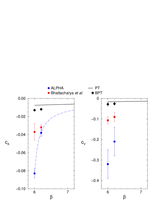
Figure 1: The improvement coefficients $c_{A}$ (left) and $c_{V}$ (right) as functions of the coupling $\beta$. Note that the vertical scales in the two plots are different. The values of the coefficients are shown for the two values of the coupling used in this work. The dashed line through the ALPHA $c_{A}$ points is their interpolating function.

The two non-perturbative determinations of the improvement coefficients give very similar values for the renormalisation coefficients ($Z$’s) and the quark mass constant $b_{V}$ (Table 2). However, the mixing coefficients $c_{A}$ and $c_{V}$ differ greatly for the two values of the coupling used here. This is shown in Figure 1. Changes in $c_{A}$ and $c_{V}$ can have a particularly large effect on the extracted values of the decay constants when the pseudoscalar and vector meson masses are not small (in lattice units), since the improved current matrix elements are given by,

$$\langle 0|A_{4}^{\mathrm{I}}|P\rangle\ = \langle 0|A_{4}|P\rangle\ +c_{A}\sinh\left(aM_{P}\right)\langle 0|P|P\rangle$$

$$\langle 0|V_{i}^{\mathrm{I}}|V,\epsilon\rangle = \langle 0|V_{i}|V,\epsilon\rangle+c_{V}\sinh\left(aM_{V}\right)\langle 0|T_{i4}|V,\epsilon\rangle$$ (13)

when the ground state is isolated. In particular at $\beta=6.0$ the heavy-light meson mass at the heaviest kappa is somewhat bigger than one such that $\sinh aM\sim 1.3$. This is illustrated for the pseudoscalar decay constant in Figure 2. The figure shows the ratio $R^{4}$ (between PA and PP correlators, defined in equation (19) and proportional to $f_{P}$), for several different values of $c_{A}$ at $\beta=6.0$. It can be seen that using the NP value of $c_{A}$ from the ALPHA collaboration decreases $R^{4}$ by $\sim 20\%$ relative to the case $c_{A}=0$. The plot also shows the ratio determined using the NP value of $c_{A}$ from Bhattacharya et al.

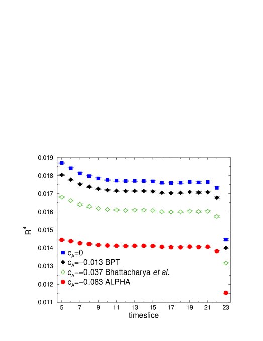
Figure 2: The mixing of the axial current with the pseudoscalar density. $\beta=6.0$, $\kappa_{H}=0.1123$, $\kappa_{L}=0.13344$. The ratio plotted is defined in equation (19).

At $\beta=6.0$ the disagreement between ALPHA and Bhattacharya et al. in the mixing coefficients is striking. Bhattacharya et al. try to estimate some of the cut-off effects in their determination of $c_{A}$ by looking at the difference between two- and three-point derivatives. They also note that since $a^{2}$ only halves between $\beta=6.0$ and $\beta=6.2$, where disagreement is substantially decreased, even higher order cut-off effects are playing a dominant rôle. Collins and Davies [27] have examined the effect of using higher-order derivatives in determining $c_{A}$ on the data set used in this work and point out that the difference in the value of $c_{A}$ from different orders of derivative disappears once the chiral limit is taken. There is clearly a large ${\mathcal{O}}(a)$ ambiguity in the value of $c_{A}$.

Bhattacharya et al. have computed all the coefficients needed for this calculation in a consistent fashion and their determinations are used here for that reason. The values of the mixing coefficients $c_{A}$ and $c_{V}$ are an order of magnitude larger in the ALPHA determinations than in BPT at $\beta=6.0$. This has a large impact on the HQS relation between, and scaling of, the decay constants. When the values of the mixing coefficients from Bhattacharya et al. are used the HQS relation is satisfied and there is good scaling.

The ALPHA collaboration compute $b_{V}$ in the SF scheme at very small quark masses and in Bhattacharya et al. the heaviest quark mass is $am_{q}\sim 0.13$. One may question whether these coefficients can be used around the charm mass: at $\beta=6.0$, $am_{c}\sim 0.75$ and at $\beta=6.2$, $am_{c}\sim 0.5$. However, the effective normalisation of the vector [28, 29] and axial [30] currents has been measured at these quark masses and found to be in good agreement with the determinations of $Z_{V}$ and $b_{V}$.

A value for $b_{m}$ is required to compute the rescaled quark mass used in the chiral extrapolations. Whilst there is a non-perturbative determination [31], it is only at one value of the coupling, and so this work follows [15] and uses the BPT value with which the non-perturbative value is consistent.

Expressions for the static improvement and renormalisation coefficients $c^{\mathrm{stat}}_{A}$, $b^{\mathrm{stat}}_{A}$ and $Z^{\mathrm{stat}}_{A}$, have been derived in perturbation theory [11],

$$Z_{A}^{\mathrm{stat}} = 1.0+\left(\frac{\ln(a\mu)}{4\pi^{2}}-0.137(1)\right)g^{2}+{\mathcal{O}}(g^{4})$$ (14)

$$b_{A}^{\mathrm{stat}} = \frac{1}{2}-0.056(7)g_{0}^{2}+{\mathcal{O}}(g_{0}^{4})$$

$$c_{A}^{\mathrm{stat}} = -\frac{1}{4\pi}\times 1.01(5)g_{0}^{2}$$

where $g_{0}$ is the bare lattice coupling. The one-loop PT and NP renormalisation schemes have been matched at the scale $\mu=m_{b}$ [32, 33] in the $\overline{\mathrm{MS}}$ scheme. The coupling $g$ is then evaluated in the $\overline{\mathrm{MS}}$ scheme [34] at the scale $m_{b}$. The values for $b^{\mathrm{stat}}_{A}$ and $c^{\mathrm{stat}}_{A}$ have been evaluated with the boosted coupling at $\beta=6.0$. The values are

$$Z_{A}^{\mathrm{stat}} = 0.663{}^{+17}_{-15}$$ (15)

$$b_{A}^{\mathrm{stat}} = 0.4057$$

$$c_{A}^{\mathrm{stat}} = -0.1354$$

where the errors on $Z_{A}^{\mathrm{stat}}$ reflect the uncertainty in $m_{b}=4.0-4.4$ GeV [34] and in the $\overline{\mathrm{MS}}$ coupling.

2.6 Extraction of masses and decay constants of heavy-light mesons

The pseudoscalar meson masses are extracted from the asymptotic behaviour of the two-point correlation functions,

$$C_{PP}^{SS}(t,\vec{p}) = \sum_{\vec{x}}e^{-i\vec{p}{\cdot}\vec{x}}\langle\Omega_{P}^{S}(t,\vec{x})\Omega_{P}^{S\dagger}(0,\vec{0})\rangle$$

$$\stackrel{{\scriptstyle t\to\infty}}{{\to}} {\left(Z^{S}_{P}(\vec{p})\right)^{2}\over 2aE_{P}}\cosh(aE_{P}(t-T/2))e^{-aE_{P}T/2}$$

where $T=48$ and $aE_{P}$ is the energy of the lowest lying meson destroyed by the operator $\Omega^{S}_{P}$ and created by $\Omega_{P}^{S\dagger}$. The superscript $S$ denotes a smeared, or spatially extended, interpolating field operator constructed using the gauge invariant technique described in [35]. $Z_{P}^{S}(\vec{p})$ is the overlap of the operator with the pseudoscalar state given by $Z_{P}^{S}(\vec{p})$ = $\langle 0|\Omega_{P}^{S}(0,\vec{0})|{\mathrm{P}}(\vec{p})\rangle$. Fit ranges are established by inspection of the time-dependent effective mass. Table 3 shows the best fit masses in each case. A similar procedure is used to extract the masses of vector mesons from correlation functions constructed with the appropriate vector operators.

Table 3: Pseudoscalar and vector masses in lattice units at $\beta=6.2$ and $\beta=6.0$. Fit ranges are $12-22$ at $\beta=6.2$ and $10-22$ (P), $10-21$ (V) at $\beta=6.0$.

$\beta=6.2$
$\kappa_{\mathrm{H}}$	$\kappa_{\mathrm{L}}$	$aM_{P}$	$aM_{V}$
	$0.1346$	$0.841^{+1}_{-1}$	$0.871^{+2}_{-2}$
$0.1200$	$0.1351$	$0.823^{+2}_{-1}$	$0.856^{+2}_{-2}$
	$0.1353$	$0.817^{+2}_{-1}$	$0.848^{+3}_{-2}$
	$0.1346$	$0.739^{+1}_{-1}$	$0.775^{+2}_{-2}$
$0.1233$	$0.1351$	$0.721^{+2}_{-1}$	$0.759^{+2}_{-2}$
	$0.1353$	$0.714^{+2}_{-1}$	$0.752^{+3}_{-2}$
	$0.1346$	$0.628^{+1}_{-1}$	$0.673^{+2}_{-2}$
$0.1266$	$0.1351$	$0.609^{+1}_{-1}$	$0.656^{+2}_{-2}$
	$0.1353$	$0.602^{+2}_{-1}$	$0.650^{+3}_{-2}$
	$0.1346$	$0.505^{+1}_{-1}$	$0.563^{+2}_{-2}$
$0.1299$	$0.1351$	$0.484^{+1}_{-1}$	$0.546^{+2}_{-2}$
	$0.1353$	$0.476^{+1}_{-1}$	$0.540^{+2}_{-2}$

$\beta=6.0$
$\kappa_{\mathrm{H}}$	$\kappa_{\mathrm{L}}$	$aM_{P}$	$aM_{V}$
	$0.13344$	$1.145^{+2}_{-1}$	$1.188^{+2}_{-2}$
$0.1123$	$0.13417$	$1.121^{+2}_{-2}$	$1.166^{+3}_{-3}$
	$0.13455$	$1.110^{+3}_{-2}$	$1.158^{+4}_{-4}$
	$0.13344$	$1.006^{+2}_{-1}$	$1.056^{+2}_{-2}$
$0.1173$	$0.13417$	$0.981^{+2}_{-2}$	$1.034^{+3}_{-2}$
	$0.13455$	$0.969^{+2}_{-2}$	$1.026^{+4}_{-4}$
	$0.13344$	$0.851^{+1}_{-1}$	$0.915^{+2}_{-2}$
$0.1223$	$0.13417$	$0.825^{+2}_{-1}$	$0.892^{+3}_{-2}$
	$0.13455$	$0.811^{+2}_{-2}$	$0.883^{+4}_{-3}$
	$0.13344$	$0.675^{+1}_{-1}$	$0.759^{+2}_{-2}$
$0.1273$	$0.13417$	$0.646^{+2}_{-1}$	$0.736^{+3}_{-2}$
	$0.13455$	$0.631^{+2}_{-1}$	$0.727^{+4}_{-3}$

The decay constants are extracted from the large time behaviour of different two-point correlation functions at zero momentum. The PA correlation function is used for the pseudoscalar decay constant:

$$C_{PA}^{SL}(t,\vec{0}) = \sum_{\vec{x}}\langle A_{4}^{\mathrm{I}}(t,\vec{x})\Omega_{P}^{S\dagger}(0,\vec{0})\rangle$$

$$\stackrel{{\scriptstyle t\to\infty}}{{\to}} \frac{Z_{A}^{L}Z_{P}^{S}}{2aM_{P}}{\sinh(aM_{P}(t-T/2))e^{-aM_{P}T/2}}$$

where $A_{4}^{\mathrm{I}}$ is the time component of the improved axial current operator defined in equation (2.1). The superscript $L$ on the correlator denotes a local operator, in this case the axial current. $Z^{L}_{A}=\langle 0|A_{4}^{\mathrm{I}}|P(\vec{0})\rangle$ is the overlap of the local axial operator with the pseudoscalar state, from which the decay constant is extracted using equations (3) and (11).

Extraction of the vector decay constant involves the large time behaviour of the VV correlation function:

$$C_{VV}^{SL}(t,\vec{0}) = \sum_{j}\sum_{\vec{x}}\langle V_{j}^{\mathrm{I}}(t,\vec{x})\Omega_{V_{j}}^{S\dagger}(0,\vec{0})\rangle$$

$$\stackrel{{\scriptstyle t\to\infty}}{{\to}} \frac{Z_{V}^{L}Z_{V}^{S}}{2aM_{V}}\cosh(aM_{V}(t-T/2))e^{-aM_{V}T/2}$$

where $V_{j}^{\mathrm{I}}$ is a spatial component of the improved local vector current operator. Again, $S$ denotes a smeared or spatially extended interpolating field operator and $L$ a local operator. The factor $Z_{V}^{L}$ is the overlap of the local vector operator with the vector state, $Z^{L}_{V}=\sum_{r}\epsilon^{r}_{k}\langle 0|V_{k}^{\mathrm{I}}|V(\vec{0},\vec{\epsilon}\,)\rangle$, from which the vector decay constant can be extracted via equation (12).

Matrix elements proportional to the decay constants can be extracted from ratios of correlation functions. The ratio

$$R^{4}\equiv\frac{C^{SL}_{PA}(t)}{C^{SS}_{PP}(t)}\stackrel{{\scriptstyle t\to\infty}}{{\to}}\frac{Z_{A}^{L}}{Z_{P}^{S}}\tanh(aM_{P}(T/2-t))$$ (19)

is used for the pseudoscalar case and is shown in Figure 2 for various values of $c_{A}$. The vector decay constant is determined using

$$\frac{C^{SL}_{VV}(t)}{C^{SS}_{VV}(t)}\stackrel{{\scriptstyle t\to\infty}}{{\to}}\frac{Z_{V}^{L}}{Z_{V}^{S}}$$ (20)

Results for the decay constants are shown in Table 4.

An alternative method is to fit several correlators simultaneously allowing an estimation of the contamination of the ground state signal by excited states. An eight-parameter fit is made to $C^{SS}_{PP}$, $C^{SL}_{PA}$ and $C^{SL}_{PP}$, allowing for ground and first excited state contributions. Results for the pseudoscalar decay constant are consistent with the single ratio fit. The ratio method is used for central values in the following but the difference from the multi-exponential fits is quoted in Table 14 below as one measure of systematic error.

Table 4: Pseudoscalar and vector decay constants in lattice units. At $\beta=6.2$ the fit ranges are $14-21$ (P) and $15-23$ (V). At $\beta=6.0$ the fit ranges are $14-21$ (P) and $16-23$ (V).

$\beta=6.2$
$\kappa_{\mathrm{H}}$	$\kappa_{\mathrm{L}}$	$af_{P}$	$f_{V}$
	$0.1346$	$0.0892^{+8}_{-8}$	$9.03^{+10}_{-\ 9}$
$0.1200$	$0.1351$	$0.0847^{+8}_{-9}$	$9.28^{+12}_{-12}$
	$0.1353$	$0.0832^{+9}_{-9}$	$9.37^{+14}_{-13}$
	$0.1346$	$0.0873^{+7}_{-8}$	$7.98^{+\ 8}_{-\ 8}$
$0.1233$	$0.1351$	$0.0829^{+7}_{-8}$	$8.17^{+10}_{-\ 9}$
	$0.1353$	$0.0814^{+8}_{-9}$	$8.23^{+11}_{-10}$
	$0.1346$	$0.0847^{+6}_{-7}$	$6.89^{+\ 6}_{-\ 6}$
$0.1266$	$0.1351$	$0.0805^{+6}_{-8}$	$7.00^{+\ 8}_{-\ 7}$
	$0.1353$	$0.0790^{+7}_{-9}$	$7.03^{+\ 9}_{-\ 8}$
	$0.1346$	$0.0804^{+6}_{-7}$	$5.76^{+\ 5}_{-\ 5}$
$0.1299$	$0.1351$	$0.0765^{+6}_{-8}$	$5.79^{+\ 6}_{-\ 5}$
	$0.1353$	$0.0751^{+6}_{-9}$	$5.79^{+\ 7}_{-\ 6}$

$\beta=6.0$
$\kappa_{\mathrm{H}}$	$\kappa_{\mathrm{L}}$	$af_{P}$	$f_{V}$
	$0.13344$	$0.1244^{+10}_{-11}$	$8.79^{+11}_{-\ 9}$
$0.1123$	$0.13417$	$0.1187^{+12}_{-13}$	$8.94^{+14}_{-12}$
	$0.13455$	$0.1167^{+15}_{-16}$	$8.89^{+19}_{-14}$
	$0.13344$	$0.1217^{+10}_{-10}$	$7.80^{+\ 9}_{-\ 8}$
$0.1173$	$0.13417$	$0.1162^{+10}_{-11}$	$7.89^{+11}_{-10}$
	$0.13455$	$0.1142^{+12}_{-14}$	$7.84^{+16}_{-11}$
	$0.13344$	$0.1170^{+\ 7}_{-\ 9}$	$6.74^{+\ 7}_{-\ 6}$
$0.1223$	$0.13417$	$0.1118^{+\ 8}_{-10}$	$6.79^{+\ 9}_{-\ 8}$
	$0.13455$	$0.1097^{+10}_{-12}$	$6.72^{+12}_{-\ 9}$
	$0.13344$	$0.1102^{+\ 6}_{-\ 9}$	$5.62^{+\ 6}_{-\ 5}$
$0.1273$	$0.13417$	$0.1053^{+\ 7}_{-\ 9}$	$5.59^{+\ 7}_{-\ 6}$
	$0.13455$	$0.1032^{+\ 8}_{-11}$	$5.51^{+\ 9}_{-\ 7}$

2.6.1 The static-light axial current

The static-light axial current can be extracted from axial-axial correlation functions. The local-local and local-smeared correlation functions were used in this work, with large-time behaviour given by

$$C_{AA}^{LL}{}(t,\vec{0}) \ =\ \sum_{\vec{x}}\left\langle A^{L}_{4}(t,\vec{x})A^{L\dagger}_{4}(0,\vec{0})\right\rangle \ \stackrel{{\scriptstyle t\to\infty}}{{\to}}\ (Z_{A}^{L})^{2}e^{-a\Delta Et}$$ (21)

$$C_{AA}^{LS}(t,\vec{0}) \ =\ \sum_{\vec{x}}\left\langle A^{S}_{4}(t,\vec{x})A^{L\dagger}_{4}(0,\vec{0})\right\rangle \ \stackrel{{\scriptstyle t\to\infty}}{{\to}}\ Z^{S}_{A}Z_{A}^{L}e^{-a\Delta Et}$$

where $\Delta E$ is the unphysical difference between the mass of the meson and the mass of the bare heavy quark. The static-light amplitude, $Z_{L}$, is

$$Z_{L}=af_{P}^{\mathrm{stat}}\sqrt{\frac{aM_{P}^{\mathrm{stat}}}{2}}$$ (22)

The smearing function is again the one described in [35].

The static-light correlation functions were generated at only one value of the coupling, $\beta=6.0$, and without the covariant derivative operators necessary to improve the current. The assumption that the matrix element of the improvement term is of the same order of magnitude as the primary term leads to ${\mathcal{O}}(10\%)$ error in the static point associated with the absence of improvement.

The signal of the static-axial current is very quickly overwhelmed by statistical noise, making the fit difficult. Simultaneously fitting to both the local-local and local-smeared correlator gives a better estimate of the local current. This is shown in Figure 3. The renormalised values of $Z_{L}$ (without the current improvement term) are shown in Table 5.

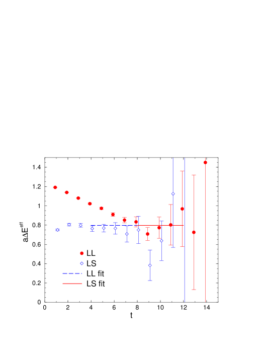
Figure 3: The effective mass plot for the LL and LS static-light axial correlation function. $\kappa_{L}=0.13344$. The lines on the plot show the value of the fit, and the fit ranges.

Table 5: Values of $a\Delta E$ and $Z_{L}$ from simultaneous fits to the LL and LS correlation functions. The fit ranges are 8-12 for the LL and 4-12 for the LS.

$\kappa_{L}$	$Z_{L}$	$a\Delta E$
0.13344	$0.30(2)$	$0.80(2)$
0.13417	$0.28(2)$	$0.78(3)$
0.13455	$0.26(3)$	$0.76(3)$

2.7 Extraction of masses and decay constants of light-light mesons

The masses and decay constants of the light-light pseudoscalar mesons are extracted from a simultaneous fit to three correlation functions: $C^{SS}_{PP}$, $C^{SL}_{PP}$ and $C^{SL}_{PA}$. The smearing function used for the light-lights is the ‘fuzzing’ of reference [36]. The results for the decay constants are shown in Table 6. The results for the pseudoscalar masses are compatible with those in [15] where a similar fit was used.

Table 6: The light-light pseudoscalar decay constants. The fit ranges are $8-22$ at both values of the coupling, except for the lightest mass combination at $\beta=6.0$ where the fit range was $7-23$.

$\beta=6.2$
$\kappa_{1}$	$\kappa_{2}$	$af_{P}$
$0.13460$	$0.13460$	$0.0640{}^{+7}_{-7}$
$0.13510$	$0.13460$	$0.0610{}^{+6}_{-7}$
$0.13530$	$0.13460$	$0.0599{}^{+6}_{-7}$
$0.13510$	$0.13510$	$0.0587{}^{+5}_{-6}$
$0.13530$	$0.13510$	$0.0575{}^{+6}_{-6}$
$0.13530$	$0.13530$	$0.0559{}^{+6}_{-7}$

$\beta=6.0$
$\kappa_{1}$	$\kappa_{2}$	$af_{P}$
$0.13344$	$0.13344$	$0.0881{}^{+10}_{-10}$
$0.13417$	$0.13344$	$0.0841{}^{+10}_{-\ 9}$
$0.13455$	$0.13344$	$0.0821{}^{+10}_{-10}$
$0.13417$	$0.13417$	$0.0798{}^{+\ 9}_{-11}$
$0.13455$	$0.13417$	$0.0775{}^{+\ 9}_{-15}$
$0.13455$	$0.13455$	$0.0730{}^{+17}_{-18}$

3 Extrapolation and interpolation in the quark masses

Extrapolation or interpolation in quark masses must be performed to extract physical masses and decay constants. For heavy quarks, the presence of ${\mathcal{O}}(a^{2}m_{Q}^{2})$ lattice artefacts when using the SW action with the NP improved renormalisation scheme imposes a constraint $am_{Q}<1$ on the quark masses that can be studied. This limits hadron masses to $\sim 2$ GeV or slightly greater at $\beta=6.0$, see Table 10. Input light quark masses are kept above $m_{\mathrm{s}}/2$ to avoid critical slowing down of quark propagator calculations and the possible appearance of finite volume effects. Interpolations to $m_{\mathrm{c}}$ and $m_{\mathrm{s}}$ are needed, together with extrapolations for $m_{\mathrm{b}}$ and the light quarks.

3.1 The light-light sector

The dependence of the light pseudoscalar decay constant on the light pseudoscalar meson mass is described by chiral perturbation theory, giving the following ansatz:

$$af_{P}=c_{0}+c_{1}(aM_{P})^{2}+c_{2}(aM_{P})^{4}$$ (23)

The value of $af_{P}$ for which

$$\frac{af_{P}}{aM_{P}}=\left(\frac{f_{\pi}}{m_{\pi}}\right)_{\mathrm{expt}}$$ (24)

can then be determined and compared to the experimental value of $f_{\pi}$, taken from [34], to fix the lattice spacing. At both values of the coupling, quadratic and linear fits in $(aM_{P})^{2}$ give essentially the same answer for the lattice spacing. Thus the data satisfy lowest-order chiral perturbation theory. Because of quenching and other systematic effects, determinations of the lattice spacing from different quantities disagree. In this work the lattice spacing is set by $f_{\pi}$. Lattice spacings fixed by the Sommer scale, $r_{0}$, [37, 38], and $m_{\rho}$ as determined by [15] are used to estimate systematic error from this source. The values are shown in Table 7.

Table 7: The inverse lattice spacing, $a^{-1}$ (GeV)

	$\beta=6.2$	$\beta=6.0$
$f_{\pi}$	$2.66{}^{+7}_{-7}$	$1.91{}^{+6}_{-6}$
$r_{0}$	$2.91{}^{+1}_{-1}$	$2.12{}^{+1}_{-1}$
$m_{\rho}$	$2.54{}^{+4}_{-9}$	$1.89{}^{+3}_{-5}$

The light, or ‘normal’, quark mass $m_{\mathrm{n}}$, defined by $m_{\mathrm{n}}\equiv(m_{\mathrm{u}}+m_{\mathrm{d}})/2$, and strange quark mass $m_{\mathrm{s}}$ are determined using the lowest-order chiral perturbation theory relation for the mass of a pseudoscalar meson with quark content $q_{1}$ and $q_{2}$,

$$(am_{\mathrm{P}})^{2}=B(a\widetilde{m}_{q_{1}}+a\widetilde{m}_{q_{2}})$$ (25)

where the rescaled quark mass $\widetilde{m}_{\mathrm{q}}$ is defined in equation (6). The value of $\kappa_{\mathrm{crit}}$ is taken from a previous UKQCD calculation [15] and is listed in Table 1. The value of the hopping parameter corresponding to the normal quark mass is set by the charged pion according to

$$a^{2}(m^{2}_{\pi})_{\mathrm{expt}}=2Ba\widetilde{m}_{\mathrm{n}}$$ (26)

and that for the strange quark mass by

$$a^{2}(m^{2}_{K})_{I}=B(a\widetilde{m}_{\mathrm{n}}+a\widetilde{m}_{\mathrm{s}})$$ (27)

where

$$(m^{2}_{K})_{I}=\frac{1}{2}(m_{K^{\pm}}^{2}+m^{2}_{K^{0}})$$ (28)

with the lattice spacing set by $f_{\pi}$. These hopping parameters are also listed in Table 1.

The ansatz for the dependence of the light pseudoscalar decay constant on quark masses is:

$$af_{P}=f_{0}+f_{1}(a\widetilde{m}_{q_{1}}+a\widetilde{m}_{q_{2}})$$ (29)

Figure 4 shows the results of fitting to this ansatz and extrapolating to $f_{\mathrm{K}}$.

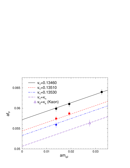
Figure 4: Dependence of the light pseudoscalar decay constant $f_{P}$ on quark masses. The lines give $f_{P}$ as a function of one of the quark masses, $a\tilde{m}_{q_{2}}$, for fixed values of the other quark mass, $a\tilde{m}_{q_{1}}$. Filled symbols are the lattice data points. The lowest line shows the extrapolation of $a\tilde{m}_{q_{1}}$ to the normal quark mass, with the open triangle giving $f_{\mathrm{K}}$ from the position of the kaon on this line.

3.2 Chiral extrapolations of heavy-light masses and decay constants

A linear dependence of heavy-light masses and decay constants on the light quark mass is assumed:

$$aK_{i}=\alpha_{i}+\beta_{i}a\widetilde{m}_{\mathrm{q}}$$ (30)

where $K_{i}$ is $f_{P}$, $f_{V}/a$, $m_{P}$ or $m_{V}$. Some example extrapolations are shown in Figure 5. The results for the extrapolated quantities are shown in Tables 8  and 9.

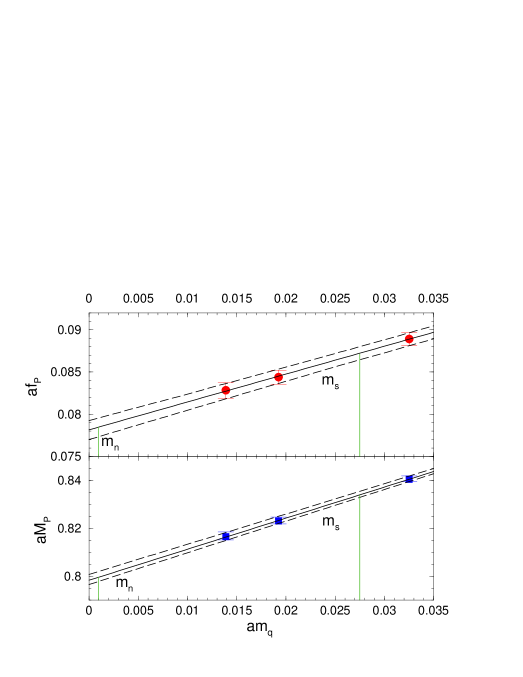
Figure 5: The chiral extrapolation of the pseudoscalar decay constant (top) and pseudoscalar mass (bottom) against rescaled light quark mass. $\beta=6.2$ and $\kappa_{H}=0.1200$. The vertical lines show the strange and normal quark masses.

Table 8: Masses and decay constants at physical light quark masses. $\beta=6.2$.

$\kappa_{H}$	$\kappa_{L}$	$aM_{P}$	$af_{P}$	$aM_{V}$	$f_{V}$
	$\kappa_{n}$	$0.800(2)$	$0.079(1)\$	$0.832(4)$	$9.6(2)$
$0.1200$	$\kappa_{s}$	$0.828(2)$	$0.0876(8)$	$0.860(2)$	$9.1(1)$
	$\kappa_{n}$	$0.696(2)$	$0.077(1)$	$0.736(3)$	$8.4(1)$
$0.1233$	$\kappa_{s}$	$0.726(1)$	$0.0857(8)$	$0.764(2)$	$8.05(9)$
	$\kappa_{n}$	$0.583(2)$	$0.075(1)$	$0.634(3)$	$7.1(1)$
$0.1266$	$\kappa_{s}$	$0.615(1)$	$0.0832(7)$	$0.661(2)$	$6.93(7)$
	$\kappa_{n}$	$0.455(2)$	$0.071(1)$	$0.523(3)$	$5.8(1)$
$0.1299$	$\kappa_{s}$	$0.491(1)$	$0.0789(7)$	$0.551(1)$	$5.77(6)$

Table 9: Masses and decay constants at physical light quark masses. $\beta=6.0$.

$\kappa_{H}$	$\kappa_{L}$	$aM_{P}$	$af_{P}$	$aM_{V}$	$f_{V}$
	$\kappa_{n}$	$1.087(4)$	$0.112(2)$	$1.138(5)$	$9.0(2)$
$0.1123$	$\kappa_{s}$	$1.125(2)$	$0.122(1)$	$1.171(3)$	$8.8(1)$
	$\kappa_{n}$	$0.945(3)$	$0.109(2)$	$1.005(5)$	$7.9(2)$
$0.1173$	$\kappa_{s}$	$0.985(2)$	$0.119(1)$	$1.039(3)$	$7.8(1)$
	$\kappa_{n}$	$0.786(3)$	$0.105(1)$	$0.862(5)$	$6.8(1)$
$0.1223$	$\kappa_{s}$	$0.829(2)$	$0.115(1)$	$0.897(3)$	$6.75(8)$
	$\kappa_{n}$	$0.603(2)$	$0.099(1)$	$0.704(5)$	$5.5(1)$
$0.1273$	$\kappa_{s}$	$0.651(2)$	$0.1080(9)$	$0.740(3)$	$5.60(7)$

3.3 Heavy quark extrapolations

Heavy Quark Symmetry (HQS) implies asymptotic scaling laws [39] for the decay constants in the infinite heavy quark mass limit. Away from this limit, heavy quark effective theory ideas motivate the following ansätze for the dependence on the heavy meson masses:

$$\Phi_{P}(M_{P}) \equiv \Theta(M_{\mathrm{B}},M_{P})f_{P}\sqrt{M}_{P}=\gamma_{P}\left(1+\frac{\delta_{P}}{M_{P}}+\frac{\eta_{P}}{M_{P}^{2}}\right)$$ (31)

$$\Phi_{V}(M_{V}) \equiv \Theta(M_{\mathrm{B}},M_{V})\frac{M_{V}}{f_{V}}\sqrt{M}_{V}=\gamma_{V}\left(1+\frac{\delta_{V}}{M_{V}}+\frac{\eta_{V}}{M_{V}^{2}}\right)$$ (32)

where $\Theta$ denotes logarithmic corrections given at leading order by [40],

$$\Theta(M_{\mathrm{B}},M)=\left(\frac{\alpha(M)}{\alpha(M_{\mathrm{B}})}\right)^{2/\beta_{0}}$$ (33)

Here, $\beta_{0}$ is the one-loop QCD beta function coefficient, equal to $11$ in the quenched approximation, and $\Lambda^{(4)}_{\overline{\mathrm{MS}}}=295$ MeV [41].

HQS also relates the pseudoscalar and vector decay constants as follows [40];

$$U(\overline{M})\equiv\frac{f_{V}f_{P}}{\overline{M}}=\left(1+\frac{8}{3}\frac{\alpha_{s}(\overline{M})}{4\pi}+{\mathcal{O}}(1/\overline{M})\right)$$ (34)

where $\overline{M}\equiv(M_{P}+3M_{V})/4$ is the spin-averaged heavy meson mass. The one-loop factor $\Theta$ in equations (31) and (32) cancels in the ratio in equation (34). Higher-order QCD corrections produce the term proportional to $\alpha_{\mathrm{s}}$. $\widetilde{U}(\overline{M})$ is defined to eliminate the radiative corrections in $U(\overline{M})$,

$$\widetilde{U}(\overline{M})\equiv U(\overline{M})/\left\{1+\frac{8}{3}\frac{\alpha_{\mathrm{s}}(\overline{M})}{4\pi}\right\}$$ (35)

Calculated values of $\widetilde{U}(\overline{M})$ are fitted to the following parameterisation:

$$\widetilde{U}(\overline{M})=\omega_{0}+\frac{\omega_{1}}{\overline{M}}+\frac{\omega_{2}}{\overline{M}^{2}}$$ (36)

HQS implies that $\omega_{0}=1$. However, $\omega_{0}$ can also be left as a free parameter to test the applicability of HQS. Likewise, HQS can be applied to set $\gamma_{P}=\gamma_{V}$ in fits using equations (31) and (32). However, higher order QCD corrections would modify this in a similar way to $\widetilde{U}(\overline{M})$, that is

$${\gamma_{P}\over\gamma_{V}}=\left(1+\frac{8}{3}\frac{\alpha_{s}(\overline{M})}{4\pi}\right)$$ (37)

The systematic error arising from extrapolating the decay constants to the $b$ mass is studied in Section 4. The error from truncating the expansion in inverse powers of the heavy mass is considered and the issue of the propagation of discretisation effects under this extrapolation is addressed.

4 Decay constants

The main results for the decay constants are listed in Table 11 and summarised in the introduction. Central values are obtained at $\beta=6.2$, setting the scale with $f_{\pi}$. These results are discussed in more detail here, starting with $f_{\mathrm{K}}$.

For $f_{\mathrm{K}}$ the largest source of uncertainty is the choice of quantity used to set the scale. The value of $f_{\mathrm{K}}$ increases by $8\%$ when the scale is set by $r_{0}$ and decreases by $4\%$ when it is set by $m_{\rho}$. When $m_{\phi}$ is used to fix the strange quark mass rather than $m_{\mathrm{K}}$, the value of $f_{\mathrm{K}}$ decreases by $2.5\%$. With only two values of the lattice spacing a continuum extrapolation is not attempted. The decay constant is smaller at $\beta=6.0$ by $2.7\%$, which is taken as an estimate of its discretisation error. These estimates of systematic errors are combined in quadrature.

The ALPHA collaboration [42] have computed the decay constant, $f_{\mathrm{K}}$, with the same action as used here, at several values of the coupling. They perform a continuum extrapolation of $r_{0}f_{\mathrm{K}}$ against $a^{2}/r_{0}^{2}$. To examine the scaling behaviour of the decay constant in this work, a comparison with the ALPHA results is shown in Figure 6. The line shows the linear extrapolation to the continuum limit (CL) that was performed by ALPHA, excluding the point at the coarsest lattice spacing, $\beta=6.0$. There are two main differences in the calculations. First, ALPHA use degenerate light quark masses, whereas this work specifically takes into account the non-degeneracy of the quarks. However, ALPHA have checked on the same dataset analysised in this work that using degenerate light quarks has negligible effect. A more obvious difference is in the values of the improvement coefficients, $c_{A}$ and $b_{A}$. As noted earlier, improvement coefficients may differ by ${\mathcal{O}}(a)$ terms, depending on the improvement condition used. A particular choice of conditions used to determine the coefficients may result, for a particular quantity, in smaller discretisation effects at finite lattice spacing. This seems to be the case for the decay constants when the improvement coefficients of Bhattacharya et al. are used rather than those determined by ALPHA, especially at $\beta=6.0$. However, as the continuum limit is approached the values of $f_{\mathrm{K}}$ from the two studies converge.

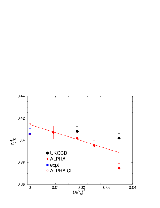
Figure 6: The dependence of $f_{K}$ on the lattice spacing.

The major source of uncertainty in the heavy-light decay constants comes from the determination of the lattice spacing. Additional systematic errors arise from discretisation effects and from the heavy quark extrapolations. Since these latter errors are related to the size of the heavy quark masses, the heavy masses used in this work are listed in Table 10. All these errors will now be discussed.

Table 10: Heavy quark and meson masses used in this work. The table shows the bare quark mass in lattice units, the renormalisation group invariant quark mass defined by $m^{\mathrm{RI}}_{Q}=Z_{m}(1+b_{m}am_{Q})m_{Q}$[43] in GeV and the heavy-light($\kappa_{n}$) pseudoscalar meson mass in GeV. The scale is set by $f_{\pi}$.

$\beta=6.2$
$\kappa$	$am_{Q}$	${m}^{\mathrm{RI}}_{Q}$	$M_{P}$
0.1200	0.485	1.59	$2.128(5)$
0.1233	0.374	1.36	$1.851(5)$
0.1266	0.268	1.06	$1.551(5)$
0.1299	0.168	0.72	$1.210(5)$

$\beta=6.0$
$\kappa$	$am_{Q}$	${m}^{\mathrm{RI}}_{Q}$	$M_{P}$
0.1123	0.756	1.26	$2.076(8)$
0.1173	0.566	1.18	$1.805(6)$
0.1223	0.392	0.97	$1.501(6)$
0.1273	0.231	0.65	$1.152(4)$

Table 11: The decay constants at both $\beta$ values with the scale set by $f_{\pi}$,$r_{0}$ and $m_{\rho}$ and a quadratic (Q) or linear (L) fit for the extrapolation in inverse heavy meson mass. The quadratic fit uses all four heavy masses, while the linear fit uses the heaviest three. The central values are shown in bold face.

		$\beta=6.2$				$\beta=6.0$
		$f_{P}$(MeV)		$f_{V}$		$f_{P}$(MeV)		$f_{V}$
		Q	L	Q	L	Q	L	Q	L
	B	${\bf 195(6)}$	$178(5)$	$28(1)$	$29(1)$	$200(8)$	$182(7)$	$26(2)$	$28(2)$
	D	${\bf 206(4)}$	$207(4)$	$\ 8.6(3)$	$\ 8.6(3)$	$210(4)$	$211(5)$	$\ 8.3(3)$	$\ 8.3(3)$
$f_{\pi}$	$\mathrm{B_{s}}$	${\bf 220(6)}$	$201(5)$	$25.2(8)$	$26.5(8)$	$222(7)$	$202(7)$	$25(1)$	$26(1)$
	$\mathrm{D_{s}}$	${\bf 229(3)}$	$230(4)$	$8.3(2)$	$\ 8.3(2)$	$230(4)$	$230(4)$	$\ 8.3(2)$	$\ 8.3(2)$
	B	$217(5)$	$200(4)$	$24.8(8)$	$25.9(7)$	$226(6)$	$207(5)$	$18.9(8)$	$20.4(8)$
	D	$222(3)$	$223(3)$	$\ 7.8(2)$	$\ 7.8(2)$	$229(3)$	$230(3)$	$\ 6.7(2)$	$\ 6.8(2)$
$r_{0}$	$\mathrm{B_{s}}$	$240(4)$	$222(3)$	$22.9(5)$	$24.0(4)$	$247(4)$	$226(3)$	$21.9(7)$	$23.1(5)$
	$\mathrm{D_{s}}$	$243(2)$	$244(2)$	$7.7(1)$	$\ 7.7(1)$	$246(2)$	$247(2)$	$\ 7.5(1)$	$\ 7.5(1)$
	B	$185(4)$	$168(3)$	$29.5(9)$	$31.1(9)$	$197(6)$	$179(4)$	$26(1)$	$28(1)$
	D	$199(3)$	$199(3)$	$\ 9.1(2)$	$\ 9.1(2)$	$208(3)$	$209(3)$	$\ 8.4(2)$	$\ 8.4(2)$
$m_{\rho}$	$\mathrm{B_{s}}$	$209(3)$	$191(2)$	$26.5(5)$	$28.0(4)$	$220(3)$	$200(2)$	$24.9(7)$	$26.5(5)$
	$\mathrm{D_{s}}$	$221(2)$	$222(2)$	$\ 8.7(1)$	$\ 8.7(1)$	$228(2)$	$228(2)$	$\ 8.4(1)$	$\ 8.4(1)$

The ambiguity in the decay constants from the lattice spacing is quite large: there is an overall $16\%$ variation in the value of $f_{\mathrm{B}}$ when the scale is set by $m_{\rho}$, $r_{0}$ or $f_{\pi}$ (see Table  11). The difference between the decay constants determined at $\beta=6.2$ and $\beta=6.0$ is smallest when the scale is set by $f_{\pi}$, as shown in Figure 7. This is not surprising since some systematic uncertainties may cancel in ratios of decay constants. Therefore the central values are quoted using $f_{\pi}$ to set the scale.

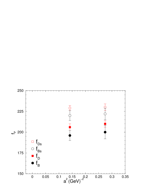
Figure 7: The dependence of the pseudoscalar decay constants on the lattice spacing. The scale is set by $f_{\pi}$.

Discretisation errors are considered next. Although this calculation is ${\mathcal{O}}(a)$ improved, ${\mathcal{O}}(a^{2})$ effects may still be important at any fixed lattice spacing. In particular, ${\mathcal{O}}(a^{2}m^{2})$ effects could well be significant for heavy quarks. With results at only two values of the lattice spacing, a full continuum extrapolation cannot be attempted. The heavy-light decay constant at the finer lattice spacing is taken as the central value, with the result at the coarser spacing used as one indicator of discretisation errors. A fuller investigation of discretisation effects for the heavy quarks follows.

The general characteristic size of discretisation effects in this simulation is investigated by examining the free particle dispersion relation, which is altered in discrete spacetime. The lattice dispersion relation can be written

$$E^{2}=M_{1}^{2}+\frac{M_{1}}{M_{2}}\vec{p}^{\ 2}+{\mathcal{O}}(p^{4})$$ (38)

where $M_{1}$ is the energy at zero momentum and $M_{2}$ is the kinetic mass, defined by $M_{2}^{-1}=\left.\partial^{2}E/\partial p_{i}^{2}\right|_{\vec{p}=0}$. The dispersion relation is investigated by fitting hadronic correlators computed at five different momentum values ($\vec{p}^{\;2}=0,1,2,3,4$ in lattice units) using linear and quadratic fits in $\vec{p}^{\;2}$. The fit for the heaviest quark combination at $\beta=6.0$ is shown on the left of Figure 8. For lighter mass combinations at $\beta=6.0$ the signal for highest momentum is very poor, and so in general the fits exclude the $|\vec{p\;}|^{2}=4$ channel. The right hand side of Figure 8 shows the $M_{1}/M_{2}$ estimates for each heavy quark.

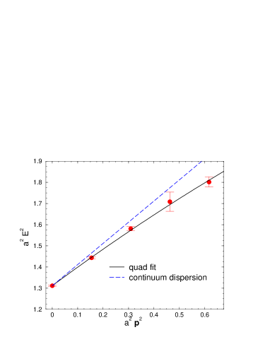
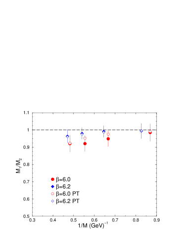
Figure 8: Left: the pseudoscalar dispersion relation for $\kappa_{H}=0.1123$, $\kappa_{L}=0.13344$ in lattice units at $\beta=6.0$. Right: the ratio $M_{1}/M_{2}$ as a function of $M_{1}$.

Also shown on the right in Figure 8 is the ratio of $M_{1}/M_{2}$ when $M_{2}$ has been determined by the shift in quark mass from $m_{1}$ to $m_{2}$ [44].

$$M_{2}^{\mathrm{PT}}=M_{1}+(m_{2}-m_{1})$$ (39)

and the quark masses $m_{1}$ and $m_{2}$ have been calculated from the tree-level relation described in  [7, 45, 46].

$$am_{1}=\ln(1+am_{Q})$$ (40)

$$\frac{1}{am_{2}}=\frac{2}{am_{Q}(2+am_{Q})}+\frac{1}{1+am_{Q}}$$ (41)

Here $M$ denotes hadron mass and $m$ denotes quark mass. There is good agreement between the tree-level perturbative description of $M_{2}$ and the NP determination. At the quark masses used in this work the ratio $M_{1}/M_{2}$ remains close to unity, so that deviations from the continuum dispersion relation are small. Finally, it is worth noting that $M_{2}$ is determined at non-zero momentum, which is statistically noiser, and so has statistical errors an order of magnitude larger than for $M_{1}$.

The axial current in this work is normalised according to equations (2.1,3). As already mentioned the improvement term is proportional to $\sinh(aM_{P})$ and the mass-dependent normalisation is proportional to $am_{Q}$. Bernard [9] proposed the following alternative normalisation, labelled CB,

$$(A_{0}^{R})_{\mathrm{CB}}=Z_{A}\left[1+b_{A}a\bar{m}+2ac_{A}\frac{\partial_{0}\langle 0|P|P\rangle}{\bar{m}\langle 0|A_{0}|P\rangle}\right]^{1/2}A_{0}$$ (42)

where $\bar{m}$ is the average of the bare quark masses in the heavy-light state. The CB normalisation differs from the NP improvement scheme normalisation only at ${\mathcal{O}}(a^{2})$. Taking into account an additional normalisation of $\sqrt{4\kappa_{Q}\kappa_{q}}$, the CB norm has a finite static limit since $\kappa_{Q}am_{Q}\to 1/2$ in as $\kappa_{Q}\to 0$. The CB norm looks very like the normalisation of Kronfeld, Lepage and Mackenzie (KLM norm) [7, 26, 45, 46],

$$\psi\to\psi^{\prime}=\psi\sqrt{1+\mu am}$$ (43)

where $\mu$ would be the mean link in the tadpole improved tree-level Fermilab formalism. In this case $\mu$ is a mass-dependent factor that contains the information about improving the current.

Figure 9 shows the mass dependence of the function $\Phi$, defined in equation (31), for a variety of methodologies. The NP norm is shown with both a quadratic fit (Q) to all four masses and a linear (L) fit to the heaviest three. The CB norm data has the extrapolation using the $M_{2}$ masses rather than $M_{1}$. It is clear from the figure that the difference between the “NP Q vs $M_{1}$” and “CB Q vs $M_{2}$” fits is smaller than the difference between the quadratic and linear fits to NP norm. It should be noted that the effect of changing the normalisation to CB differs from that described in [9] which used the ALPHA determination of $c_{A}$ and the preliminary NP determination by Bhattacharya et al.  [22] of $b_{A}$.

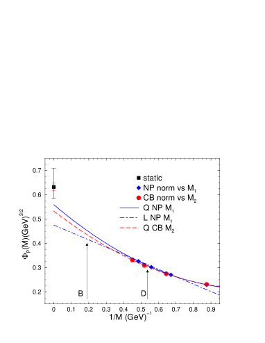
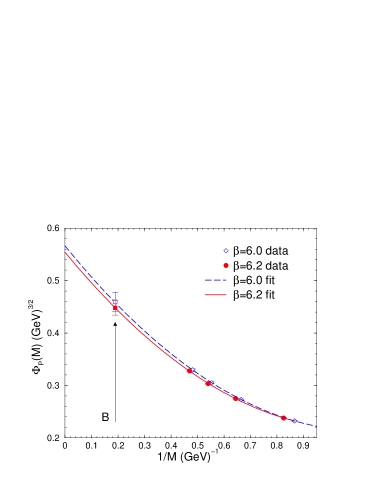
Figure 9: The left plot shows the extrapolations of the pseudoscalar decay constant in heavy meson mass at $\beta=6.0$ with different normalisations and masses. The right plot shows a comparison between the extrapolations at both values of the coupling.

In the ${\mathcal{O}}(a)$ improved theory used here, ${\mathcal{O}}(a^{2}m_{Q}^{2})$ lattice artefacts could still be large: the worst case simulated has $a^{2}m_{Q}^{2}\sim 0.5$ (see Table 10) and one may worry that mass-dependent discretisation effects, which may not be too large at the charm scale, are enhanced by extrapolation to the bottom scale. Although a Taylor expansion of $(am_{Q})^{2}$ in $1/m_{Q}$ around the charm quark mass needs large terms to reproduce $(am_{b})^{2}$, the issue is not directly the fate of ${\mathcal{O}}(a^{2}m_{Q}^{2})$ under extrapolation, but rather the effect of such terms at the charm scale on the extrapolation.

The left hand plot in Figure 9 includes the static point. The smaller set of error bars shows the error from renormalisation, the larger, the statistical uncertainty. The static point is higher than the extrapolations; however, the missing static improvement term would lower the static point, since $c_{A}^{\mathrm{stat}}$ is negative. For this reason an interpolation to the $b$ quark mass using the static and $c$ quark data is not implemented; rather the static point is used as a check of the extrapolation. The result supports the view that, the increase in discretisation error after the heavy quark extrapolation is moderate.

The right-hand side of Figure 9 shows the extrapolation of $\Phi_{P}$ for both values of $\beta$ in physical units. Although the difference between the curves does indeed grow during the extrapolation, it is smaller than the statistical errors at the bottom scale. The qualitative agreement between the two curves suggests that discretisation errors are not large. To study this further, equation (31) is modified as follows,

$$\Phi(M,a)=\gamma\left(1+\frac{\delta}{M}+\frac{\eta}{M^{2}}+\varepsilon(aM)^{2}+\zeta(aM)^{3}\right)$$ (44)

and data from both lattice spacings fitted simultaneously. This uses the two values of $a$ to increase the number of $aM$ values available, allowing the important class of heavy-mass dependent discretisation errors to be studied. The sum of the first three terms in equation (44) has these errors subtracted out and is hereafter referred to as the ‘quasi-continuum’ result. Figure 10 shows the quasi-continuum curve as a function of $1/M$, together with $\Phi(M,a)$ at each $\beta$ value separately. The curves A and B which blow up as $1/M\to 0$ are the fits to equation (44) containing lattice artefacts. However, the quasi-continuum result, where these artefacts are subtracted, does not differ greatly from the extrapolations at the individual lattice spacings using equation (31). The quasi-continuum $\Phi$ gives $f_{B}=186(10)$ MeV, which differs by $5\%$ at $\beta=6.2$ (the number appearing in Table 14) and $7\%$ at $\beta=6.0$ from the extrapolations using (31). Excluding the $\zeta$ term, or using $am_{Q}$ instead of $aM$ makes little difference. Using $(aM)^{2}\Lambda/M$ instead of $(aM)^{2}$ also makes no significant difference. Varying all five fit parameters in equation (44) over the region where the chi-squared per degree of freedom increases by up to $1$ from its minimum value gives a variation of $\pm 16$ MeV for the quasi-continuum $f_{B}$, so the fit is stable.

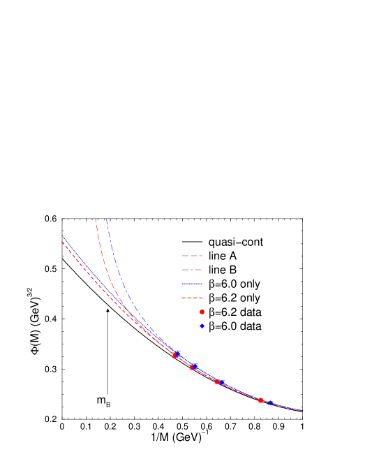
Figure 10: Effects of lattice artefacts on the heavy quark extrapolation. The solid line shows the quasi-continuum extrapolation described in the text. The dashed and dotted lines show $\Phi$, equation (31), when extrapolating at each value of $\beta$ separately. Line A(B) shows the function $\Phi(M,a)$, equation (44), at $\beta=6.2(6.0)$.

The systematic error associated with truncating the HQET series is now discussed. First, linear and quadratic fits to the data are compared. The linear fit uses the heaviest three quark masses and drops the $\eta$ term from equations (31) and (32). This is compared to a quadratic fit using all four masses. The resulting variations, which are shown in Table 11, amount to a relative error of $9\%$ for $f_{\mathrm{B}}$, indicating that a quadratic term is necessary. A cubic fit is performed to check that a quadratic term is sufficient. There are not enough data points for a cubic fit at each lattice spacing, so the fit combines data from both lattices as before, adding a cubic term $\xi/M^{3}$ to $\Phi(M,a)$. This results in a value of $f_{\mathrm{B}}$ which is $5\%$ greater than the quasi-continuum determination. This is also included as a systematic error in Table 14.

The HQS relation between the pseudoscalar and vector decay constants can also be investigated. The quantity $\widetilde{U}(\overline{M})$ defined in equation (35) should be equal to unity in the static limit. The extrapolation of $\widetilde{U}(\overline{M})$ is shown in Figure 11 and displayed in Table 12. “Q” denotes a quadratic fit to all heavy quarks whereas “L” denotes a linear fit to the heaviest three. The extrapolation for $\beta=6.0$ displays the expected static limit, albeit with large errors. At $\beta=6.2$, $\widetilde{U}(\overline{M})$ from the quadratic fit deviates from unity in the static limit. On the finer lattice, discretisation errors are smaller and so one might expect better agreement in the static limit. However, $\widetilde{U}(\overline{M})$ depends on the ratio of the axial to vector currents and is particularly sensitive to the mixing coefficients, $c_{A}$ and $c_{V}$, which are the most poorly known of the improvement coefficients. Different determinations of $c_{V}$ vary by an order of magnitude, even at $\beta=6.2$, where all the other coefficients are in much better agreement. Indeed, varying $c_{V}$ by the quoted errors of $25\%$ in Bhattacharya et al. varies the value of $\widetilde{U}(\overline{M}_{\infty})$ by around $6\%$. Taking into account the uncertainty in the value of $c_{V}$, the value of $\widetilde{U}(\overline{M}_{\infty})$ is consistent with unity.

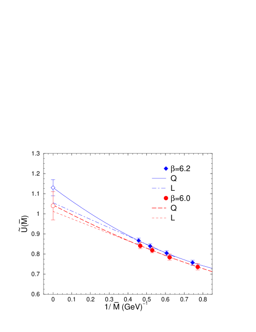
Figure 11: The quantity $\widetilde{U}(\overline{M})$ as a function of the inverse spin averaged mass $\overline{M}$.

Table 12: $\widetilde{U}(\overline{M})$ as a function of heavy meson mass.

$\beta$		$\overline{M}_{\mathrm{D}}$	$\overline{M}_{\mathrm{B}}$	$\overline{M}_{\infty}$
	Q	$0.83(1)$	$1.01(2)$	$1.13(4)$
$6.2$	L	$0.83(1)$	$0.98(2)$	$1.05(5)$
	Q	$0.82(2)$	$0.96(4)$	$1.04(7)$
$6.0$	L	$0.82(2)$	$0.94(3)$	$1.01(4)$

The $SU(3)$ flavour breaking ratios are determined by two methods: from the ratio of extrapolated values of the decay constants, labelled (i) in Table 13, or by extrapolating the ratios constructed at each heavy mass, labelled (ii) in the Table. In the ratio of $f_{P_{\mathrm{s}}}/f_{P_{\mathrm{n}}}$ most of the heavy quark mass dependence seems to cancel. The fact that the two methods agree, within statistical errors, suggests that the systematic error in these ratios is small.

Table 13: Flavour-breaking ratios.

$\beta$		$\frac{f_{\mathrm{B_{s}}}}{f_{\mathrm{B}}}$	$\frac{f_{\mathrm{D_{s}}}}{f_{\mathrm{D}}}$	$\frac{f_{\mathrm{B^{\ast}}}}{f_{\mathrm{B_{s}^{\ast}}}}$	$\frac{f_{\mathrm{D^{\ast}}}}{f_{\mathrm{D_{s}^{\ast}}}}$
	(i)	$1.13(1)$	$1.11(1)$	$1.10(2)$	$1.04(1)$
$6.2$	(ii)	$1.11(2)$	$1.11(1)$	$1.10(2)$	$1.05(1)$
	(i)	$1.11(2)$	$1.09(1)$	$1.05(3)$	$1.00(2)$
$6.0$	(ii)	$1.10(2)$	$1.09(1)$	$1.05(3)$	$1.01(2)$

The systematic variations of the decay constants are shown in Table 14, in order of importance. The total systematic uncertainty is obtained by combining these in quadrature.

Table 14: Percentage systematic uncertainties. Systematic differences are obtained by varying the procedure used to calculate the decay constants. The central values are fixed by using $f_{\pi}$ to set the scale at $\beta=6.2$, performing a quadratic heavy quark extrapolation, taking the central values of the mixing coefficients $c_{A,V}$, fitting correlation functions to a single exponential, and using $m_{\mathrm{K}}^{2}$ to set the strange quark mass.

Pseudoscalar	$f_{\mathrm{B}}$	$f_{\mathrm{D}}$	$f_{\mathrm{B_{s}}}$	$f_{\mathrm{D_{s}}}$	$\frac{f_{\mathrm{B_{s}}}}{f_{\mathrm{B}}}$	$\frac{f_{\mathrm{D_{s}}}}{f_{\mathrm{D}}}$
scale set by $r_{0}$	$11$	$8$	$9$	$6$	$-2$	$-2$
scale set by $m_{\rho}$	$-5$	$-3$	$-5$	$-3$	$1$	$1$
linear vs quadratic	$-9$	$-$	$-9$	$-$	$-$	$-$
quasi-continuum	$-5$	$-2$	$-5$	$-2$	$-$	$-$
quasi-continuum plus $1/M^{3}$	$5$	$-$	$5$	$-$	$-$	$-$
$\beta=6.0$	$3$	$2$	$1$	$1$	$-1$	$-2$
multi-exp	$-2$	$-3$	$-5$	$-3$	$-3$	$1$
strange quark mass from $m_{\phi}$	$-$	$-$	$-2$	$-2$	$-2$	$-2$
coeff. $c_{\mathrm{A}}$	$1$	$1$	$1$	$1$	$1$	$-$
Vector	$f_{\mathrm{B^{\ast}}}$	$f_{\mathrm{D^{\ast}}}$	$f_{\mathrm{B_{s}^{\ast}}}$	$f_{\mathrm{D_{s}^{\ast}}}$	$\frac{f_{\mathrm{B^{*}}}}{f_{\mathrm{B^{*}_{s}}}}$	$\frac{f_{\mathrm{D^{*}}}}{f_{\mathrm{D^{*}_{s}}}}$
scale set by $r_{0}$	$-11$	$-10$	$-9$	$-8$	$2$	$2$
scale set by $m_{\rho}$	$6$	$5$	$5$	$5$	$1$	$1$
$\beta=6.0$	$-7$	$-4$	$-2$	$-1$	$-5$	$-4$
linear vs quadratic	$5$	$-$	$5$	$-$	$-$	$-$
quasi-continuum	$6$	$3$	$6$	$3$	$-$	$-$
quasi-continuum plus $1/M^{3}$	$-5$	$-$	$-5$	$-$	$-$	$-$
strange quark mass	$-$	$-$	$2$	$2$	$-3$	$-2$
coeff $c_{V}$	$3$	$1$	$3$	$1$	$1$	$1$

4.1 Comparison with other determinations

A comparison with some other recent quenched results for $f_{\mathrm{B}}$ is shown in Table 15. For a comprehensive review, the reader is referred to the article by Bernard [9]. The results which use the Fermilab formalism [7] are continuum limits. The APE result uses the same action at $\beta=6.2$ and the UKQCD Tad result uses the same gauge configurations as this work but with a tadpole improved value of $c_{\mathrm{SW}}$.

Table 15: Comparison with some other recent determinations of $f_{\mathrm{B}}$. “FNAL” denotes use of the Fermilab formalism [7] and “charm” indicates that the heavy quarks have masses around charm and are then extrapolated to the bottom scale. NB: the World Average is not the average of the numbers displayed below.

	Heavy Quark	$f_{\mathrm{B}}$ (MeV)
El-Khadra et al. [47]	FNAL	$164(8){}^{+11}_{-\ 8}$
MILC [48, 49]	FNAL	$173(6){}^{+16}_{-16}$
JLQCD [50]	FNAL	$173(4)(9)(9)$
UKQCD Tad [51]	charm	$177(17){}^{+22}_{-26}$
APE [52]	charm	$179(18){}^{+34}_{-\ 9}$
CP-PACS [53]	FNAL	$188(3)(9)$
This Work	charm	$195(6){}^{+24}_{-23}$
World Average [9]		$175(20)$

The value of $f_{\mathrm{B}}$ obtained in this work is the highest, although it is compatible with the world average. One reason for this might be the heavy quark method employed. However, other results using the same heavy quark extrapolation have a lower value, while the most recent result using the Fermilab method from the CP-PACS collaboration [53] has a value in agreement within statistical errors. Different heavy quark methods have different associated systematic uncertainties. A detailed analysis of those present in this work has been discussed above, including an estimate of the effects of the heavy quark extrapolation. These uncertainties are also explored in [9], which additionally addresses some of the systematic issues affecting the Fermilab formalism. The value obtained in this work is consistent within these systematic uncertainties with other quenched results.

There have been several recent calculations of $f_{\mathrm{B}}$ with two flavours ($N_{F}=2$) of dynamical fermions using NRQCD or the Fermilab formalism. Again, they are reviewed in [9]. The effect of unquenching is found to increase the value of $f_{\mathrm{B}}$ by $10-15\%$.

The only heavy-light decay constant to have been measured experimentally so far is $f_{\mathrm{D_{s}}}$ [54],

$$f_{\mathrm{D_{s}}}=260\pm 19\pm 32\ \mathrm{MeV}$$ (45)

With such large uncertainties, the experimental value is consistent with both the unquenched and quenched values of $f_{\mathrm{D_{s}}}$.

5 Spectroscopic quantities

To determine the value of the hopping parameter, $\kappa_{c}$, corresponding to the charm quark mass requires an interpolation in heavy quark mass. The improved quark mass definition in equation (6) also applies to heavy quarks, so if the meson mass depends linearly on the improved heavy quark mass, the corresponding bare quark mass dependence is,

$$aM_{\mathrm{H}}(m_{Q})=\rho+\lambda am_{Q}+\epsilon a^{2}m_{Q}^{2}$$ (46)

where $\epsilon/\lambda=b_{m}$. In the NP improved formulation all lattice artefacts of ${\mathcal{O}}(a)$ have been removed. However, ${\mathcal{O}}(a^{2}m_{Q}^{2})$ effects for the heaviest quarks could be significant. Any contributions at this order would affect the ratio $\epsilon/\lambda$ such that it was no longer equal to $b_{m}$. A fit to equation (46) was tried with $\epsilon/\lambda$ fixed to $b_{m}$ from boosted perturbation theory, and with $\epsilon/\lambda$ allowed to vary freely. The heavy quark dependence can be used to fix $\kappa_{\mathrm{c}}$ by choosing a particular state (or splitting) to have its physical value. Choosing the pseudoscalar mass to fix $\kappa_{\mathrm{c}}$, the spectrum of heavy-light mesons can then be predicted.

For $\beta=6.2$, the results of using equation (46) are shown in Figure 12. Whilst the value of $\epsilon/\lambda=-0.505(4)$ (labelled FIT in the figure) differs somewhat from the value of $b_{m}=-0.652$ from BPT, it makes little difference to the value of the $\kappa_{\mathrm{c}}$, of order $0.1\%$. The choice of quantity to set the lattice spacing clearly has a rather large effect. Values for $\kappa_{\mathrm{c}}$ are shown in Table 16, using the free fit to set the value of the hopping parameter.

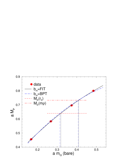
Figure 12: The pseudoscalar meson vs. bare quark mass for $\beta=6.2$

Table 16: The hopping parameter corresponding to the charm quark mass. The label FIT refers to the ratio $\epsilon/\lambda$ in equation (46) having a fitted value, whilst BPT refers to the ratio having the BPT value.

	$\beta=6.2$		$\beta=6.0$
$a^{-1}$	FIT	BPT	FIT	BPT
$a^{-1}(r_{0})$	$0.12498^{+6}_{-5}$	$0.12513^{+6}_{-5}$	$0.11952^{+8}_{-6}$	$0.12056^{+8}_{-6}$
$a^{-1}(m_{\rho})$	$0.12221^{+7}_{-5}$	$0.12227^{+7}_{-5}$	$0.1160^{+1}_{-1}$	$0.1165^{+2}_{-2}$
$a^{-1}(f_{\pi})$	$0.1232^{+6}_{-5}$	$0.1233^{+6}_{-6}$	$0.1164^{+10}_{-11}$	$0.1171^{+3}_{-10}$

For $\beta=6.0$, the fitted value of $\epsilon/\lambda=-0.384(3)$ differs significantly from the value of $b_{m}=-0.662$ from BPT. Consequently the fit using the BPT $b_{m}$ has a very large $\chi^{2}$, as the data cannot accomodate a model with such large curvature. However, the difference in $\kappa_{\mathrm{c}}$ is still small (of order $1\%$). For $\beta=6.2$ the heaviest quark has a value of $am_{Q}=0.485$ whereas for $\beta=6.0$ the heaviest quark has $am_{Q}=0.775$. Discretisation errors of ${\mathcal{O}}(a^{2}m^{2})$ could be responsible for modifying the value of the ratio $\epsilon/\lambda$. The value of $\kappa_{\mathrm{c}}$ is rather insensitive to $\epsilon/\lambda$ but because the value of $am_{\mathrm{Q}}$ is so large, the improved quark mass changes dramatically. Using the free fit as the preferred method, the value of $\kappa_{\mathrm{c}}$ is shown in Table 16.

The spectrum of heavy-light charm states is shown in Figure 13 and tabulated in Table 17. With only two values of $\beta$ a continuum extrapolation is not attempted, but the difference between the two couplings can be used to estimate systematic errors. It is clear from the figure that a large systematic error arises from the definition of the lattice spacing. Depending on which quantity is chosen, different mass splittings appear to be closer to their continuum values. The central values for the spectrum are produced by the following procedures: single exponential fits, using $r_{0}$ to set the scale, with $\epsilon/\lambda$ a free parameter in equation (46). The values of the masses at $\beta=6.2$ are taken to be the central values, with the values at $\beta=6.0$ used to estimate systematic error. The remaining estimates of systematic error come from using multiple exponential fits, using $m_{\rho}$ to set the scale and, in the case of states with a strange quark, using $m_{\mathrm{K}^{*}}$ instead of $m_{\mathrm{K}}^{2}$ to set the strange quark mass. All these systematic errors are combined in quadrature. The results, with experimental comparisons, are:

$$\begin{array}[]{rcl}\lx@intercol\hfil\mbox{Lattice, this work}\hfil\lx@intercol\\ M_{\mathrm{D}_{\mathrm{s}}}&=&1.956^{+2}_{-2}\ {}^{+22}_{-\ 4}\,\mathrm{GeV}\\ M_{\mathrm{D}^{*}}&=&2.002^{+7}_{-6}\ {}^{+16}_{-41}\,\mathrm{GeV}\\ M_{\mathrm{D}^{*}_{\mathrm{s}}}&=&2.082^{+4}_{-5}\ {}^{+22}_{-31}\,\mathrm{GeV}\end{array}\qquad\qquad\begin{array}[]{rcl}\lx@intercol\hfil\mbox{Experiment~{}\cite[cite]{[\@@bibref{}{pdg2000}{}{}]}}\hfil\lx@intercol\\ M_{\mathrm{D}^{+}_{\mathrm{s}}}&=&1.9685^{+5}_{-5}\,\mathrm{GeV}\\ M_{\mathrm{D}^{*0}}&=&2.0067^{+5}_{-5}\,\mathrm{GeV}\\ M_{\mathrm{D}^{*+}_{\mathrm{s}}}&=&2.1124^{+7}_{-7}\,\mathrm{GeV}\end{array}$$ (47)

For the lattice results, the first error is statistical and the second systematic. In this calculation the light quark in each meson is a normal quark. Thus the $\mathrm{D}^{*}$ is the isospin-averaged vector state, with mass $M_{\mathrm{D}^{*}}=(M_{\mathrm{D}^{*0}}+M_{\mathrm{D}^{*\pm}})/2$. With somewhat large systematic errors, the largest of which comes from the lattice spacing, the spectrum is in broad agreement with experiment.

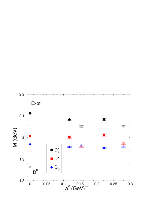
Figure 13: The scaling of the D meson spectrum. The filled symbols have the lattice spacing set by $r_{0}$, and the open symbols by $m_{\rho}$.

Table 17: The spectrum of heavy-light mesons with different definitions of the lattice spacing in GeV.

state	$a^{-1}$	$\beta=6.2$	$\beta=6.0$
	$r_{0}$	$1.956^{+2}_{-2}$	$1.952^{+2}_{-2}$
$\mathrm{D}_{\mathrm{s}}$	$m_{\rho}$	$1.963^{+2}_{-3}$	$1.958^{+3}_{-3}$
	$f_{\pi}$	$1.960^{+4}_{-4}$	$1.958^{+4}_{-3}$
	$r_{0}$	$2.002^{+7}_{-6}$	$2.011^{+8}_{-7}$
$\mathrm{D}^{*}$	$m_{\rho}$	$1.960^{+6}_{-6}$	$1.973^{+7}_{-6}$
	$f_{\pi}$	$1.973^{+10}_{-10}$	$1.977^{+14}_{-14}$
	$r_{0}$	$2.082^{+4}_{-5}$	$2.083^{+4}_{-4}$
$\mathrm{D}^{*}_{\mathrm{s}}$	$m_{\rho}$	$2.052^{+3}_{-4}$	$2.053^{+4}_{-3}$
	$f_{\pi}$	$2.061^{+7}_{-7}$	$2.056^{+10}_{-10}$

It is also of interest to look at the $M_{V}-M_{P}$ splitting as a function of the (pseudoscalar) meson mass. This can be extrapolated in inverse mass to the B scale, and to the infinite quark mass limit where the splitting should vanish. The splittings at both values of $\beta$ are given in Table 18 and are plotted for $\beta=6.2$ in Figure 14. There is little difference between linear and quadratic fits, so only the linear fit is shown. The splittings obtained from the linear fit at $\beta=6.2$, using $r_{0}$ to set the scale, are taken as the central values quoted below. The second set of errors is systematic, obtained by combining in quadrature the differences arising from the following variations in procedure (in descending order of importance): using $m_{\rho}$ rather than $r_{0}$ to set the scale; (for the B meson) using a quadratic rather than linear extrapolation; multiple rather than single exponential fits; using $\beta=6.0$ data rather than $\beta=6.2$ data. The results, with the comparison to experiment, are as follows:

$$\begin{array}[]{rcl}\lx@intercol\hfil\mbox{Lattice, this work}\hfil\lx@intercol\\ M_{\mathrm{D}^{*}}-M_{\mathrm{D}}&=&130^{+6}_{-6}{}^{+15}_{-35}\ \mathrm{MeV}\\ M_{\mathrm{B}^{*}}-M_{\mathrm{B}}&=&\ 21^{+7}_{-8}{}^{+18}_{-16}\ \mathrm{MeV}\end{array}\quad\quad\begin{array}[]{rcl}\lx@intercol\hfil\mbox{Experiment~{}\cite[cite]{[\@@bibref{}{pdg2000}{}{}]}}\hfil\lx@intercol\\ M_{\mathrm{D}^{*}}-M_{\mathrm{D}}&=&142.6\pm 0.5\ \mathrm{MeV}\\ M_{\mathrm{B}^{*}}-M_{\mathrm{B}}&=&\ 45.2\pm 1.8\ \mathrm{MeV}\end{array}$$ (48)

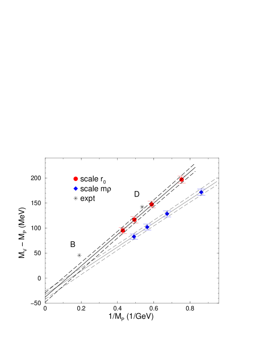
Figure 14: The hyperfine splitting as a function of $M$ in physical units at $\beta=6.2$. The circles have the scale set by $r_{0}$ and the diamonds by $m_{\rho}$.

Table 18: The hyperfine splitting of the heavy-light mesons at the B and D meson scale, in MeV.

state	$a^{-1}$	$\beta=6.2$	$\beta=6.0$
	$r_{0}$	$130^{+7}_{-6}$	$140\ ^{+8}_{-6}$
$M_{\mathrm{D}^{*}}-M_{\mathrm{D}}$	$m_{\rho}$	$95^{+6}_{-6}$	$108\ ^{+7}_{-6}$
	$f_{\pi}$	$105^{+9}_{-9}$	$111^{+14}_{-13}$
	$r_{0}$	$21^{+7}_{-8}$	$32\ ^{+8}_{-8}$
$M_{\mathrm{B}^{*}}-M_{\mathrm{B}}$	$m_{\rho}$	$12^{+6}_{-7}$	$22\ ^{+8}_{-8}$
	$f_{\pi}$	$15^{+8}_{-8}$	$24^{+14}_{-14}$

6 Conclusions

The decay constants of heavy-light and light mesons have been determined in the quenched approximation at two values of the coupling. The action and currents have been fully NP ${\mathcal{O}}(a)$ improved. Good scaling of the decay constants is found.

Uncertainties in the improvement and renormalisation coefficients are seen to have a large effect on the decay constants. The ALPHA and Bhattacharya et al. determinations of the improvement coefficients produce different values of $f_{\mathrm{K}}$, especially at $\beta=6.0$. However, the $f_{\mathrm{K}}$ do converge as the lattice spacing decreases. Computed quantities may well differ at ${\mathcal{O}}(a^{2})$ at fixed lattice spacing but should agree in the continuum limit.

The heavy-light decay constants are found to be around $10\%$ higher than, but compatible with, the world average [9] of quenched lattice determinations. HQS relations are found to be well satisfied by the data at both values of the coupling. The systematic uncertainties in the calculation have been discussed and, with the exception of quenching, estimated. The issue of ${\mathcal{O}}(a^{2}m^{2})$ effects in the heavy quark extrapolations has been considered in various ways. In particular, the difference of the decay constants between $\beta=6.0$ and $\beta=6.2$ at fixed heavy quark mass, as a measure of discretisation effects, is small and remains so during the heavy quark extrapolation. The static point value of the decay constant, despite the lack of improvement, suggests the extrapolation is under control. Furthermore, HQS relations are satisfied and there is agreement between $f_{\mathrm{B_{s}}}/f_{\mathrm{B}}$ computed by extrapolating the ratio and by taking the ratio of the extrapolated decay constants.

The quenched spectrum of D mesons has been determined, shows good scaling, and is found to be in broad agreement with experimental data.

References

- [1] M. Neubert and B. Stech, in Heavy Flavours II, Vol. 15 of Advanced Series on High Energy Physics, edited by A.J. Buras and M. Lindner (World Scientific, Singapore, 1998), Chap. 4, pp. 294–344.
- [2] M. Ciuchini, R. Contino, E. Franco, and G. Martinelli, Eur. Phys. J. C9, 43 (1999).
- [3] C. Bernard, T. Draper, G. Hockney and A. Soni, Phys. Rev. D 38, 33540 (1988).
- [4] M. Gavela et al., Phys. Lett. B 206, 113 (1988).
- [5] E. Eichten, Nucl. Phys. B (Proc. Suppl.) 4, 170 (1988).
- [6] G. Lepage and B. Thacker, Nucl. Phys. B (Proc. Suppl.) 4, 199 (1987).
- [7] A.X. El-Khadra, A.S. Kronfeld, and P.B. Mackenzie, Phys. Rev. D 55, 3933 (1997).
- [8] A.S. Kronfeld, Phys. Rev. D 62, 014505 (2000).
- [9] C. Bernard, Nucl. Phys. B (Proc. Suppl.) 94, 159 (2001).
- [10] B. Sheikholeslami and R. Wohlert, Nucl. Phys. B 259, 572 (1985).
- [11] M. Kurth and R. Sommer, Nucl. Phys. B 597, 488 (2001).
- [12] M. Creutz, Phys. Rev. D 36, 2394 (1987).
- [13] F. Brown and T. Woch, Phys. Rev. Lett. 58, 163 (1987).
- [14] N. Cabibbo and E. Marinari, Phys. Lett. B 119, 387 (1982).
- [15] UKQCD Collaboration, K.C. Bowler et al., Phys. Rev. D 62, 054506 (2000).
- [16] B. Efron, SIAM Review 21, 460 (1979).
- [17] M. Lüscher, S. Sint, R. Sommer and P. Weisz, Nucl. Phys. B 478, 365 (1996).
- [18] M. Lüscher, S. Sint, R. Sommer, P. Weisz, H. Wittig and U. Wolff, Nucl. Phys. B (Proc. Suppl.) 53, 905 (1997).
- [19] M. Lüscher, S. Sint, R. Sommer, and H. Wittig, Nucl. Phys. B 491, 344 (1997).
- [20] R. Sommer, Nucl. Phys. Proc. Suppl 60A, 279 (1998).
- [21] M. Guagnelli and R. Sommer, Nucl. Phys. B (Proc. Suppl.) 63A-C, 886 (1998).
- [22] T. Bhattacharya et al., Phys. Lett. B 461, 79 (1999).
- [23] T. Bhattacharya, R. Gupta, W. Lee, S. Sharpe, Nucl. Phys. B (Proc. Suppl.) 83-84, 851 (2000).
- [24] T. Bhattacharya, R. Gupta, W. Lee, S. Sharpe, Phys. Rev. D 62, 074505 (2001).
- [25] S. Sint and P. Weisz, Nucl. Phys. B 502, 251 (1997).
- [26] G. Lepage and P. Mackenzie, Phys. Rev. D 48, 2250 (1993).
- [27] S. Collins and C.T.H Davies, Nucl. Phys. B (Proc. Suppl.) 94, 608 (2001).
- [28] UKQCD Collaboration, K.C. Bowler et al., Phys. Lett. B 486, 111 (2000).
- [29] UKQCD Collaboration, C.M. Maynard, Nucl. Phys. B (Proc. Suppl.) 94, 367 (2001).
- [30] UKQCD Collaboration, in preparation.
- [31] G.M. de Divitiis and R. Petronzio, Phys. Lett. B 419, 311 (1998).
- [32] M. Kurth, private communication.
- [33] R. Sommer, Phys. Rept. 275, 1 (1996).
- [34] D.E. Groom et al., Eur. Phys. J. C 15, 1 (2000).
- [35] P. Boyle, hep-lat/9903033.
- [36] P. Lacock, A. McKerrell, C. Michael, I.M. Stopher and P.W. Stephenson, Phys. Rev. D 51, 6403 (1995).
- [37] R. Sommer, Nucl. Phys. B411, 839 (1994).
- [38] M. Guagnelli, R. Sommer and H. Wittig, Nucl. Phys. B 535, 389 (1998).
- [39] M. Neubert, Phys. Rev. D 45, 2451 (1992).
- [40] M. Neubert, Phys. Rev. D 46, 1076 (1992).
- [41] S. Bethke, Nucl. Phys. B (Proc. Suppl.) 54A, 314 (1997).
- [42] J. Garden, J. Heitger, R. Sommer and H. Wittig, Nucl. Phys. B 571, 237 (2000).
- [43] S. Capitani, M. Lüscher, R. Sommer, H. Wittig, Nucl. Phys. B 544, 669 (1999).
- [44] C. Bernard, J. Labrenz and A. Soni, Phys. Rev. D 49, 2536 (1994).
- [45] G.P. Lepage, Nucl. Phys. B (Proc. Suppl.) 26, 45 (1992).
- [46] A. Kronfeld, Nucl. Phys. B (Proc. Suppl.) 30, 445 (1993).
- [47] A.X. El-Khadra et al., Phys. Rev. D 58, 014506 (1998).
- [48] C. Bernard et al., Phys. Rev. Lett. 81, 4812 (1998).
- [49] C. Bernard et al., Nucl. Phys. B (Proc. Suppl.) 94, 346 (2001).
- [50] A. Aoki et al., Phys. Rev. Lett. 80, 5711 (1998).
- [51] UKQCD Collaboration, L. Lellouch and C.J.D. Lin, hep-ph/0011086.
- [52] D. Becirevic et al., Phys. Rev. D 60, 074501 (1999).
- [53] CP-PACS Collaboration, A. Ali Khan et al., hep-lat/0010009.
- [54] F. Muheim, private communication.