CERN-TH/2000-196
IFIC-00/41
FTUV-00-0712
A note on the practical feasibility of domain-wall fermions

Abstract

Domain-wall fermions preserve chiral symmetry up to terms that decrease exponentially when the lattice size in the fifth dimension is taken to infinity. The associated rates of convergence are given by the low-lying eigenvalues of a simple local operator in four dimensions. These can be computed using the Ritz functional technique and it turns out that the convergence tends to be extremely slow in the range of lattice spacings relevant to large-volume numerical simulations of lattice QCD. Two methods to improve on this situation are discussed.

Introduction

The idea to realize 4-dimensional (4D) chiral fermions on the lattice by coupling 5D fermions to a 4D domain wall [1] has attracted a lot of attention in the lattice community (for a review see [2]). Although originally designed to construct chiral gauge theories, the idea can also be applied to lattice QCD in order to preserve the global chiral symmetry at zero quark mass [3, 4]. In this case, a 5D Wilson–Dirac operator is chosen with $N$ slices in the extra dimension and appropriate Dirichlet boundary conditions in the fifth dimension. In the limit $N\rightarrow\infty$, chiral zero modes exist as surface modes on the 4D boundaries, even at finite lattice spacing.

The bulk fermionic degrees of freedom are massive and can be shown to decouple in the continuum limit: the action of the 5D system is equivalent to the one corresponding to a 4D Dirac operator describing the boundary chiral modes [5]; similarly, the propagator of the boundary fields can be obtained from the inverse of the same 4D operator [6]. The chirality of the surface modes in the limit $N\rightarrow\infty$ then follows [6] from the fact that, in this limit, this 4D Dirac operator satisfies the Ginsparg–Wilson (GW) relation [7]–[9], which implies an exact lattice chiral symmetry [10]. Thus the 5D domain-wall construction in the limit $N\rightarrow\infty$ is completely equivalent to a 4D lattice formulation of Ginsparg–Wilson fermions, and satisfies all the properties that follow from the exact chiral symmetry [8, 11, 12, 10, 13]. Moreover, if the continuum limit is taken in the extra dimension, this 4D formulation coincides with that using Neuberger’s fermion operator [14, 9].

The introduction of an extra dimension makes domain-wall fermions more demanding numerically than standard Wilson fermions (the equivalent 4D formulation is similarly more demanding, owing to the non-ultralocality of the action). Nevertheless the advantage of preserving an exact chiral symmetry might compensate for the higher cost in some cases. An analysis in the free theory showed that the convergence to the exact operator as a function of $N$ is rapid [3, 15]. This gave rise to the hope that also in the interacting case domain-wall fermions could be used without too much computational overhead. However, in realistic simulations, there are indications that the convergence rate deteriorates rapidly at large values of the gauge coupling, and much larger values of $N$ are indeed needed [16]–[18], leading to a substantial computational cost.

In a recent paper [19], the problems found in practical simulations were traced back to the appearance of very small eigenvalues of a certain 4D operator, which control the rate of convergence in $N$. We have performed an independent study and confirm the analysis in [19]. In addition, we discuss a new method to improve the domain-wall fermion operator, which differs from the one proposed in [19] and proves to work better numerically.

Five dimensional theory

In this section we establish our notation and collect some useful formulae, the derivation of which can be found in [3, 4, 5, 6, 20]. The 5D domain wall operator we consider here is defined as

$$\mathcal{D}=\frac{1}{2}\left\{\gamma_{5}(\partial_{s}^{*}+\partial_{s})-a_{s}\partial_{s}^{*}\partial_{s}\right\}+M,\;$$ (1)

where $s$ denotes a lattice site in the fifth direction ($a_{s}\leq s\leq a_{s}N$), $a_{s}$ is the corresponding lattice spacing, and $\partial_{s}^{*}$ and $\partial_{s}$ are the usual forward and backward derivatives. The operator $M$ in eq. (1) is obtained from the standard 4D Wilson operator by

$$M=D_{\mathrm{w}}-m_{0}$$ (2)

with

$$D_{\mathrm{w}}=\frac{1}{2}\left\{\gamma_{\mu}(\nabla_{\mu}^{*}+\nabla_{\mu})-a\nabla_{\mu}^{*}\nabla_{\mu}\right\}.\;$$ (3)

Here $\nabla_{\mu}^{*}$ and $\nabla_{\mu}$ are the gauge covariant forward and backward derivatives and $a$ is the lattice spacing in the four physical dimensions $\mu=1,...,4$. The mass parameter $m_{0}$ obeys

$$m_{0}>0,\;\;\;a_{s}m_{0}<2,\;\;\;am_{0}<2.\;$$ (4)

Note that the lattice spacings $a_{s}$ and $a$ can be different. The boundary conditions are fixed through

$$P_{+}\psi(0,x)=P_{-}\psi(a_{s}N+a_{s},x)=0\;,$$ (5)

where $P_{\pm}\equiv\frac{1}{2}(1\pm\gamma_{5})$.

Appropriate interpolating fields for the quarks constructed out of the left and right boundary modes are

$$q(x) = P_{-}\psi(a_{s},x)+P_{+}\psi(Na_{s},x)\;,$$ (6)

$$\bar{q}(x) = \bar{\psi}(a_{s},x)P_{+}+\bar{\psi}(Na_{s},x)P_{-}.$$ (7)

A mass term can then be introduced by adding to eq. (1) the term

$$\frac{1}{2}m\left\{\bar{\psi}(a_{s},x)P_{+}\psi(Na_{s},x)+\bar{\psi}(Na_{s},x)P_{-}\psi(a_{s},x)\right\}\;.$$ (8)

The two-point function of the quark fields is related to an effective 4D operator $D_{N}$ by [6]

$$\langle q(x)\bar{q}(x)\rangle=\frac{2-aD_{N}}{aD_{m,N}},$$ (9)

with

$$D_{m,N}=(1-\frac{1}{2}am)D_{N}+m.$$ (10)

In terms of the operators $K_{\pm}$,

$$K_{\pm}\equiv\frac{1}{2}\pm\frac{1}{2}\gamma_{5}\frac{a_{s}M}{2+a_{s}M},\;$$ (11)

$D_{N}$ is given by

$$aD_{N}=1+\gamma_{5}\frac{K_{+}^{N}-K_{-}^{N}}{K_{+}^{N}+K_{-}^{N}}.$$ (12)

From eq. (12) it is straightforward to show that

$$aD\equiv\lim_{N\rightarrow\infty}aD_{N}=1+\gamma_{5}\epsilon(K_{+}-K_{-})\;,$$ (13)

which can also be written as [20]

$$aD = 1-A(A^{\dagger}A)^{-1/2}$$ (14)

$$A = -a_{s}M(2+a_{s}M)^{-1}\;.$$ (15)

It follows easily from this expression that $D$ satisfies the Ginsparg–Wilson relation, the only difference to Neuberger’s operator being the different definition of $A$. Indeed, Neuberger’s operator is readily obtained from eqs. (14) and (15) by taking the limit $a_{s}\rightarrow 0$.

Similarly, in the limit $N\rightarrow\infty$, the fermion determinant of the 5D formulation can be written in terms of the determinant of $D_{m,N}$, up to local subtractions. The 5D formulation is thus completely equivalent to a 4D lattice formulation of Ginsparg–Wilson fermions satisfying an exact chiral symmetry.

A final necessary condition for this formulation to be an acceptable regularization of QCD is that the operator of eq. (14) is local. Indeed, it has been shown by Kikukawa [21] that both the operators in eqs. (14) and (12) are exponentially localized for smooth enough gauge fields, satisfying a plaquette bound [22, 23].

In realistic simulations of domain-wall fermions, $N$ is finite. In this situation, the chiral symmetry is broken by the residual terms $\delta D\equiv D_{N}-D$. It may be speculated that one could include a small additive quark mass renormalization, in order to get rid of these chirality breaking effects. This is, however, only justified by universality arguments if the subleading corrections in $N$ in the action are local. The result of [21] shows that this is indeed the case since $\delta D$ is also local. However it is important to stress that the exponential localization of $\delta D$ only sets in at distances of $\mathrm{O}(N)$. This can be shown already in the free case. On the other hand, in practical simulations the typical lattice sizes used are not much larger than $N$ and consequently $\delta D$ is not local at the distances probed. In this situation, a quark mass renormalization cannot cancel the chirality-breaking effects induced by $\delta D$.

The convergence rate in $N$

For gauge field configurations with a restricted plaquette value, the operator $A^{\dagger}A$ has a spectral gap [22]:

$$0<u\leq A^{\dagger}A\leq v,$$ (16)

ensuring the exponential convergence in $N$ of $D_{N}$. The minimum rate of convergence is given by

$$\omega=\mathrm{min_{i}}[\omega_{i}],\;\;\;\;\;\omega_{i}\equiv\mathrm{ln}\frac{1+\sqrt{\lambda_{i}}}{|1-\sqrt{\lambda_{i}}|},$$ (17)

where $\lambda_{i}$ are the eigenvalues of $A^{\dagger}A$.

However, in realistic simulations the plaquette bound is not satisfied and it is important to study the convergence rate $\omega$ for the values of $\beta$ and $m_{0}$ at which large-scale numerical simulations are performed nowadays.

The eigenvalues $\lambda$, which determine $\omega$, can be obtained through the generalized 4D eigenvalue equation

$$a_{s}^{2}M^{\dagger}M\psi=\lambda(2+a_{s}M)^{\dagger}(2+a_{s}M)\psi.\;$$ (18)

It is either the minimum or maximum eigenvalue of $A^{\dagger}A$ that minimizes $\omega_{i}$. These eigenvalues can be obtained by minimizing (maximizing) the generalized Ritz functional

$$\frac{\langle\psi|a_{s}^{2}M^{\dagger}M|\psi\rangle}{\langle\psi|(2+a_{s}M)^{\dagger}(2+a_{s}M)|\psi\rangle}\;$$ (19)

using a straightforward generalization of the algorithm described in [24] .

Eigenvalues above the lowest one can be computed by modifying the operator $M^{\dagger}M$ in the numerator of eq. (19) in such a way that the already computed eigenvalues are shifted to larger values. For example, this can be achieved by substituting $M^{\dagger}M$ by $M^{\dagger}M+\sum_{i}\alpha_{i}M^{\dagger}M|\psi_{i}\rangle\langle\psi_{i}|(2+a_{s}M)^{\dagger}(2+a_{s}M)$ with $\alpha_{i}\equiv(1-\lambda_{i})/\lambda_{i}$ and $\lambda_{i}$, $\psi_{i}$ being the already computed eigenvalues and vectors. Notice that in this method no inversion of the matrix $(2+a_{s}M)^{\dagger}(2+a_{s}M)$ is needed.

We have studied numerically the convergence rate in the quenched approximation. We find that it is always controlled by the lowest eigenvalue $\lambda_{\mathrm{min}}$ of $A^{\dagger}A$. In Figs. 1 and 2 we show the inverse convergence rates $\omega_{i}^{-1}$ corresponding to the five lowest eigenvalues of $A^{\dagger}A$ at $\beta=5.85$ on an $8^{3}\cdot 16$ lattice, and at $\beta=6.0$ on a $16^{3}\cdot 32$ lattice, respectively. In both cases we have set $a_{s}m_{0}=am_{0}=1.8$, which is a typical value used in previous simulations.

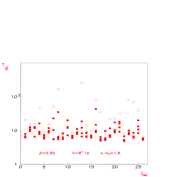
Figure 1: Inverse convergence rate $\omega_{i}^{-1}$ for the five lowest eigenvalues of $A^{\dagger}A$ (open symbols correspond to the lowest eigenvalue) as a function of Monte Carlo time $t_{\rm MC}$, at $\beta=5.85$ on an $8^{3}\cdot 16$ lattice.

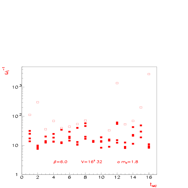
Figure 2: The same as Fig. 1 at $\beta=6$ on a $16^{3}\cdot 32$ lattice.

Figures 1 and 2 give a rather pessimistic view of the convergence of domain-wall fermions to the exact operator: they imply that several hundred or even thousand slices in the extra dimension would be needed to achieve a reasonable approximation. Clearly, this would render domain-wall fermions impracticable. Our results are consistent with the findings in [19].

It should be noted, however, that a very similar situation was found for Neuberger’s operator [22]. Also in this case very small eigenvalues of the corresponding $A^{\dagger}A=M^{\dagger}M$ occur, turning the computation of its inverse square root extremely costly.

Acceleration of convergence

In the case of Neuberger’s operator, the bad convergence behaviour resulting from the low-lying eigenvalues of $M^{\dagger}M$ could be cured by treating these modes exactly [25, 26]. It is natural to look for a similar trick also for domain-wall fermions, given the similarity of the two constructions. We have found two ways of achieving this. The first method is equivalent to the one described in [19], so we will not give any details here. The corresponding improved 5D operator differs from the standard one by boundary terms.

We have tested the inversion of this improved operator, $\mathcal{D}_{\mathrm{impr}}$, by solving the linear equation $\mathcal{D}_{\mathrm{impr}}X=Y$ for a given source $Y$. As a numerical solver we have used a conjugate gradient method with a stopping criterion $\|r\|/\|X\|<\epsilon$, where $r=\mathcal{D}_{\mathrm{impr}}X-Y$ is the residual vector and $\epsilon$ was set to $\epsilon=10^{-8}$. We found that when using such a relatively low value of $\epsilon$ the conjugate gradient method behaves very poorly: for a number of configurations at $\beta=5.85$ on an $8^{3}\cdot 16$ lattice, the norm of the residual vector developed a very long tail at rather small values of $\|r\|\leq\mathrm{O}(10^{-5})$. This resulted in a very large number of iterations in the conjugate gradient algorithm before it converged to the desired accuracy. We suspect that some subtle cancellations occur in the improved operator leading to unexpectedly large rounding error effects.

Since this behaviour of the conjugate gradient algorithm was rather unsatisfactory, we developed an alternative improvement method. The key observation for the new improved 5D operator is that the relations in eq. (15) and eq. (14) hold true for any choice of $M$ as long as

$$M^{\dagger}=\gamma_{5}M\gamma_{5}\;,\;\;\;\mathrm{det}(2+a_{s}M)\neq 0\;.$$ (20)

This fact may be used to construct an improved $M$ for which the very low eigenvalues of $A^{\dagger}A$ disappear. A possible form of $M$ that achieves this is given by

$$a_{s}\hat{M}=a_{s}M-\sum_{k,l=1}^{r}X_{kl}w_{k}\otimes w_{l}^{\dagger}\gamma_{5},\;$$ (21)

where

$$\gamma_{5}Av_{k}=\alpha_{k}v_{k},\;\;\;\;\;k=1,\cdots,r,\;\;\;\;\;(v_{k},v_{l})=\delta_{kl}\;.$$ (22)

and

$$w_{k}=(2+a_{s}M)\gamma_{5}v_{k}.$$ (23)

Finally

$$(X^{-1})_{kl}=2\delta_{kl}(\hat{\alpha}_{k}-\alpha_{k})^{-1}+(v_{k},(2+a_{s}M)\gamma_{5}v_{l})\;.$$ (24)

The corresponding 5D operator $\hat{\cal D}$ is given by eq. (1) after substituting $M$ by $\hat{M}$. Notice that the improved operator differs from the original one also in the bulk and not just at the boundary.

After some algebra it can be shown that

$$\hat{A}\equiv-a_{s}\hat{M}(2+a_{s}\hat{M})^{-1}=A+\sum_{k=1}^{r}(\hat{\alpha}_{k}-\alpha_{k})\gamma_{5}v_{k}\otimes v_{k}^{\dagger}\;.$$ (25)

It is now easy to see that $\gamma_{5}\hat{A}$ has the same eigenvectors as $\gamma_{5}A$, but all eigenvalues $\alpha_{k},\;k=1,\cdots,r,$ are replaced by $\hat{\alpha}_{k}$. The limit $N\rightarrow\infty$ of the corresponding improved 4D operator ${\hat{D}}_{N}$ is the same as that of the original $D_{N}$ provided $\mathrm{sign}({\hat{\alpha}}_{k})=\mathrm{sign}(\alpha_{k})$. However, the approach to this limit is faster for ${\hat{D}}_{N}$ if the lowest eigenvalues of ${\hat{A}}^{\dagger}{\hat{A}}$, ${\hat{\lambda}}_{k}\equiv{\hat{\alpha}}^{2}_{k}$, are larger than those of $A^{\dagger}A$, i.e. if $|{\hat{\alpha}}_{k}|>|\alpha_{k}|$.

The concrete choice of $|\hat{\alpha}_{k}|$ has to be taken with some care to optimize the convergence of the inverter. For example, taking $|\hat{\alpha}_{k}|=1$ led to a bad convergence behaviour of the conjugate gradient algorithm. It is our experience that choosing $|\hat{\alpha}_{k}|$ not much higher than $|\alpha_{r}|$, $r$ being the index of the largest eigenvalue projected out, see eq. (22), leads to a normal behaviour of the conjugate gradient algorithm.

As an example of the effect of the improvement using $\hat{M}$, eq. (21), we show in Fig. 3 the behaviour of the pion propagator at zero distance $\Gamma_{\pi}(0)$ at $\beta=5.85$ on an $8^{3}\cdot 16$ lattice and for a quark mass, $am=0.1$. A similar behaviour is obtained for the pion propagator at other distances.

Figure 3: The pion propagator at zero distance as a function of $N$. The black squares are the results for the original 5D domain wall operator. The open symbols correspond to the improved operator with three and ten eigenvalues projected out. The data are obtained on an $8^{3}\cdot 16$ lattice at $\beta=5.85$ and $am=0.1$.

Already the projection of only three low-lying eigenvalues is sufficient to accelerate the convergence substantially: similar approximations to the $N\rightarrow\infty$ limit are obtained for $N\sim 150$ in the unimproved case and $N\sim 30$ in the improved one. It would, of course, be interesting to see the effect also on other physical quantities.

Conclusions

In this note we presented numerical evidence that in practical simulations domain wall fermions need an unacceptably large number of slices in the extra dimension to ensure that the chiral symmetry-breaking terms are suppressed. The reason is that very small eigenvalues of a 4D operator appear, which are directly related to the convergence rate of the 5D domain-wall operator. These results confirm the findings in [19].

As in the case of Neuberger’s operator, it is possible, however, to separate a number of eigenvalues of the 4D operator and treat them exactly or shift them to larger harmless values. We tested two different implementations of this idea. The first has already appeared in [19], the second, which is described in detail above, is new. We found that numerically the second implementation works much better.

It is our overall impression, however, that there is no particular advantage in using domain-wall fermions instead of Neuberger’s operator. Theoretical considerations demonstrate that both approaches to realize a chiral symmetry on the lattice are equivalent, to the extent that they satisfy the Ginsparg–Wilson relation. However, in practical applications, it is our present experience that it is easier to control chiral symmetry violations with Neuberger’s operator.

Acknowledgements
We would like to thank Giulia de Divitiis for her help at an early stage of this project and the computer centres at NIC (Jülich) and CIEMAT (Madrid) for providing computer time and technical support.

References

- [1] D.B. Kaplan, Phys. Lett. B288 (1992) 342.
- [2] T. Blum, Nucl. Phys. (Proc.Suppl.) B73 (1999) 167.
- [3] Y. Shamir, Nucl. Phys. B406 (1993) 90.
- [4] V. Furman and Y. Shamir, Nucl. Phys. B439 (1995) 54.
- [5] H. Neuberger, Phys. Rev. D57 (1998) 5417.
- [6] Y. Kikukawa and T. Noguchi, hep-lat/9902022.
- [7] P.H. Ginsparg and K.G. Wilson, Phys. Rev. D25 (1982) 2649.
- [8] P. Hasenfratz, Nucl. Phys. B (Proc.Suppl.) 63A-C (1998) 53.
- [9] H. Neuberger, Phys. Lett. B427 (1998) 353.
- [10] M. Lüscher, Phys. Lett. B428 (1998) 342.
- [11] P. Hasenfratz, V. Laliena and F. Niedermayer, Phys. Lett. B427 (1998) 125.
- [12] P. Hasenfratz, Nucl. Phys. B525 (1998) 401.
- [13] S. Chandrasekharan, Phys. Rev. D60 (1999) 074503.
- [14] H. Neuberger, Phys. Lett. B417 (1998) 141.
- [15] Y. Shamir, hep-lat/0003024.
- [16] T. Blum, A. Soni and M. Wingate, Nucl. Phys. B (Proc.Suppl.) 73 (1999) 201.
- [17] T. Blum and A. Soni, Phys. Rev. Lett. 79 (1997) 3595.
- [18] A. Ali Khan, et al. (CP-PACS Collab.), hep-lat/9909049.
- [19] R.G. Edwards and U. Heller, hep-lat/0005002.
- [20] A. Borici, Phys. Lett. B453 (1999) 46.
- [21] Y. Kikukawa, hep-lat/9912056.
- [22] P. Hernández, K. Jansen and M. Lüscher, Nucl. Phys. B552 (1999) 363.
- [23] M. Lüscher, Nucl. Phys. B538 (1999) 515.
- [24] B. Bunk, K. Jansen, M. Lüscher and H. Simma, DESY report (September 1994); T. Kalkreuter and H. Simma, Comput. Phys. Commun. 93 (1996) 33.
- [25] R.G. Edwards, U.M. Heller and R. Narayanan, Phys. Rev. D59 (1999) 094510.
- [26] P. Hernández, K. Jansen and L. Lellouch, Phys. Lett. B469(1999) 198; hep-lat/0001008.