Abstract

Using the dynamical triangulation approach we perform a numerical study of a supersymmetric random surface model that corresponds to the large $N$ limit of the four–dimensional version of the IKKT matrix model. We show that the addition of fermionic degrees of freedom suppresses the spiky world-sheet configurations that are responsible for the pathological behaviour of the purely bosonic model. We observe that the distribution of the gyration radius has a power–like tail $p(R)\sim R^{-2.4}$. We check numerically that when the number of fermionic degrees of freedom is not susy–balanced, $p(R)$ grows with $R$ and the model is not well–defined. Numerical sampling of the configurations in the tail of the distribution shows that the bosonic degrees of freedom collapse to a one–dimensional tube with small transverse fluctuations. Assuming that the vertex positions can fluctuate independently within the tube, we give a theoretical argument which essentially explains the behaviour of $p(R)$ in the different cases, in particular predicting $p(R)\sim R^{-3}$ in the supersymmetric case. Extending the argument to six and ten dimensions, we predict $p(R)\sim R^{-7}$ and $p(R)\sim R^{-15}$, respectively.

Introduction

During the last decades we have witnessed a rapid development of methods of geometrical quantization. It was triggered by the discovery of the integration measure over two-dimensional geometries which was applied in calculations of quantum amplitudes in string theory [1]. In practice, it turned out that the geometrical quantization of strings works only for either non-physical dimensions $d\leq 1$ [2], or in the critical dimension $d=10$ where the world-sheet degrees of freedom of the string decouple from the theory [1, 3].

The case of non-critical strings with $d\leq 1$ was also independently formulated in terms of a matrix model which is equivalent to the dynamical triangulations approach [4]. This method allows for calculating different topological contributions in the double scaling limit [5]. However, both the Polyakov conformal field approach and the matrix model calculations break down at $d=1$. The problems that turn up at this point, also known as the ‘$d=1$ barrier’, are attributed to instabilities of the conformal mode.

Whether it is possible to stabilize the conformal mode for surfaces embedded in physical dimensions is not yet clear. Some attempts to solve this problem have been made within the conformal field formalism [6]. Another idea is to extend dynamical triangulations to the sypersymmetric case, and to attack the problem directly in physical dimensions. By introducing supersymmetry one hopes to avoid the instabilities of bosonic surfaces that manifest as the degeneration of the world-sheet geometry into branched polymers [7].

Disrectization of supersymmetric surfaces is known to be a difficult problem. A discretization of the world-sheet supersymmetry, for example, inherits all the difficulties which appear arleady on regular lattices [8] and on top of this it introduces new problems related to the fact that the symmetry must be local [9]. Supersymmetry is broken explicitly by the lattice, and it is not clear how to ascertain whether it gets restored in the continuum limit. One encounters similar problems for the Green-Schwarz type of surfaces where one has to preserve the $\kappa$-symmetry, which is a local world-sheet symmetry [12]. One also attempted to introduce supersymmetry into the surfaces models indirectly by considering models with effective actions with extrinsic curvature terms obtained by integrating out fermions from the supersymetric theory [10]. Such discretized surfaces have been extensively studied (see e.g. [11]), but it is not clear what is nature of the critical point observed in the discretized theory and whether it can be directly related to the original supersymetric theory of continuum surfaces.

In this paper we study a model of supersymmetric surfaces that constitutes a sort of classical limit of the IKKT matrix model [13] obtained by sending the matrix size $N$ to infinity [13, 14]. The attractive feature of the surface model is that the supersymmetry is introduced in such a way that in principle the model can be straightforwardly discretized. By re-writing the IIB string action in the Schild gauge [13], one avoids the problems related to the proper treatment of the local $\kappa$-symmetry in the discretization. The action that results from this procedure has no redundant degrees of freedom left, and no local symmetry.

We investigate this model by means of the dynamical triangulation approach. Some preliminary studies in this direction were already done in [15]. We perform Monte-Carlo simulations of surfaces embedded in a 4–dimensional target space. We find a theoretical picture that explains the numerical results for $d=4$, and allows us to make some predictions for the behaviour of the ten–dimensional version of the model. The results presented here give an insight into typical geometrical features of surfaces that play an important role in the ensemble generated by the IKKT matrix model [13].

The paper is organized as follows. First we shortly recall the model and describe the discretization scheme. Then we discuss singularities of the purely bosonic model and show that they are removed by adding fermions. For the model with fermions we estimate the large $L$ behaviour of the partition function by assuming that it is dominated by tube–like configurations. We present the results of the $MC$ simulations to show that tubes do indeed dominate in the ensemble. We conclude the paper with a short discussion, concerning in particular the relation of the results to the matrix model [13, 16, 17].

The model

The action for IIB strings can be cast into the following form [13] :

$$S(g,X,\bar{\Psi},\Psi) = \int d^{2}\xi\sqrt{g}\ \left(\frac{1}{4}\{X^{\mu},X^{\nu}\}^{2}-\frac{i}{2}\bar{\Psi}\Gamma_{\mu}\{X^{\mu},\Psi\}+\lambda\right)$$ (1)

Here $g_{ab}$ is the metric tensor on the world-sheet; $X^{\mu}$ are bosonic co-ordinates in the $d$-dimensional target space; $\bar{\Psi}$ and $\Psi$ are $k$-dimensional spinors; and $\Gamma_{\mu}$ are $k\times k$ Dirac matrices. For $d=10$, the dimensionality of the spinor representation is $k=32$, and $\bar{\Psi},\Psi$ are Majorana-Weyl spinors. For $d=4$, we have $k=4$, and $\bar{\Psi},\Psi$ are Weyl spinors. The Poisson brackets in (1) are defined as

$$\{X,Y\}=\frac{1}{\sqrt{g}}\ \epsilon^{ab}\,\partial_{a}X\,\partial_{b}Y\,.$$ (2)

Based on this action the authors of [13] introduced a matrix model which was then interpreted as a constructive definition of superstring theory. The matrix model is obtained from (1) by substituting fields $X^{\mu}(\xi_{1},\xi_{2})\rightarrow A^{\mu}_{ab}$ and $\Psi(\xi_{1},\xi_{2})\rightarrow\Phi_{ab}$ by $N\times N$ traceless Hermitean matrices, and the Poisson brackets by commutators $\{,\}\rightarrow-i[,]$. The resulting theory

$${\cal S}=-\mbox{Tr}\left(\frac{1}{4}[A^{\mu},A^{\nu}]^{2}+\frac{1}{2}\bar{\Phi}\Gamma_{\mu}[A^{\mu},\Phi]-\lambda\mathbbm{1}\right)$$ (3)

is quantized by the Feynman integral

$$Z=\int\rm{d}A\ \rm{d}\bar{\Phi}\ \rm{d}\Phi\ e^{-{\cal S}}$$ (4)

with the standard integration measure for traceless Hermitean matrices. This procedure defines a kind of third quantization of string theory, which is supposed to reproduce in a double scaling limit the sum over all topological and geometrical excitations of the world-sheet of strings [13, 14]. The original model [13] was defined in ten dimensions.

Here we will discuss the semiclassical limit of $N\rightarrow\infty$, in which the model reduces to the string theory on a fixed topology [14] with the partition function

$$Z=\int D\sqrt{g}DXD\bar{\Psi}D\Psi\,e^{-S(g,X,\bar{\Psi},\Psi)}$$ (5)

where the action is given by (1). We will concentrate for now on the case $d=4$, where we can most easily perform numerical simulations.

We use the dynamical triangulation approach to regularize the integration measure $D\sqrt{g}$. The partition function is then given by

$$Z=\sum_{N}e^{-\lambda N}z_{N}$$ (6)

where

$$z_{N}=\sum_{T\in{\cal T}_{N}}\frac{1}{C_{T}}\int\sideset{}{{}^{\prime}}{\prod}_{i}^{n}d^{4}X_{i}\sideset{}{{}^{\prime}}{\prod}_{i}^{n}d^{2}\bar{\Psi}_{i}d^{2}\Psi_{i}\ e^{-S_{T}(X_{i},\bar{\Psi}_{i},\Psi_{i})}\quad.$$ (7)

The sum runs over equilateral, oriented triangulations $T$ with $N$ triangles and $n=N/2+2$ vertices. $C_{T}$ is the symmetry factor of a given $T$, and $S_{T}$ is the discretized action on this particular triangulation. Primes on the products indicate that the zero modes were removed (see the following discussion). The fields $X_{i}$ and $\Psi_{i}$ are now located on the vertices of $T$. The action has one parameter, namely the cosmological constant $\lambda$. The continuum limit is taken by adjusting $\lambda$ in the grand-canonical partition function $Z(\lambda)$ to its critical value and sending the lattice spacing $a$ to zero. Alternatively, if one prefers to work with the ensemble of canonical partition functions $z_{N}$, one can take the continuum limit by simultaneously sending $N$ to infinity and $a$ to zero while holding the physical area of the worldsheet $A\sim Na^{2}$ fixed. This latter approach is the one we will choose here.

The discretized action consists of two terms, a purely bosonic part $S_{B}$ and a fermionic part $S_{F}$. Following the suggestions in [15], these are :

$$S_{B} = {\cal B}\sum_{\langle ijk\rangle}\left\{-\left((X_{ij}^{2})^{2}+(X_{jk}^{2})^{2}+(X_{ki}^{2})^{2}\right)\right.$$ (8)

$$\left.\ \ \ \ \ \ \ \ \ +2\left(X_{ij}^{2}X_{jk}^{2}+X_{jk}^{2}X_{ki}^{2}+X_{ki}^{2}X_{ij}^{2}\right)\right\}$$

$$S_{F} = \frac{i}{12}\sum_{\langle ij\rangle}\bar{\Psi}_{i}\Gamma_{\mu}\Psi_{j}(X_{\omega(ij)}^{\mu}-X_{\omega(ji)}^{\mu})\ .$$ (9)

In contrast to the action presented in [15], here $\bar{\Psi},\Psi$ are Weyl fermions. The first sum runs over all triangles of the triangulation, the second over all links. The constant in (8) is set to ${\cal B}=(8\sqrt{3}a^{2})^{-1}$. The operation $\omega$, when acting on an oriented link $\langle ij\rangle$, gives that neighbour of $i$ that comes after $j$ when going counterclockwise around $i$. In other words, if we denote two neighbouring oriented triangles by $\langle ijk\rangle$ and $\langle jin\rangle$, then $\omega(ij)=k$ and $\omega(ji)=n$ (see figure 1).

Figure 1: Two neighbouring, oriented triangles $\langle ijk\rangle$ and $\langle jin\rangle$, connected by the link $\langle ij\rangle$. The ‘outer’ vertices $k$ and $n$ can be accessed by the operation $\omega$ as defined in the text, with $\omega(ij)=k$ and $\omega(ji)=n$.

Two things should be noted about this action. Firstly, the bispinors $\bar{\Psi},\Psi$ in the target space have a handedness, i.e. $\Psi=\frac{1}{2}(\mathbbm{1}+\Gamma_{5})\Psi$ and $\bar{\Psi}=\bar{\Psi}\frac{1}{2}(\mathbbm{1}-\Gamma_{5})$. Using the chiral representation of the Dirac matrices in the Euclidean sector,

$$\vec{\Gamma}=\left(\begin{array}[]{ll}0&\vec{\sigma}\\ \vec{\sigma}&0\end{array}\right)\ ,\quad\Gamma_{0}=\left(\begin{array}[]{ll}0&-i\sigma_{0}\\ i\sigma_{0}&0\end{array}\right)\ ,\quad\Gamma_{5}=\left(\begin{array}[]{ll}\sigma_{0}&0\\ 0&-\sigma_{0}\end{array}\right)$$ (10)

where $\vec{\sigma}$ are the Pauli matrices and $\sigma_{0}$ is the $2\times 2$ unity matrix, we can parametrize the chiral bispinors $\bar{\Psi}$ and $\Psi$ in terms of two-component spinors $\psi,\bar{\psi}$ :

$$\bar{\Psi}=(0,\bar{\psi})\ ,\quad\Psi=\left(\begin{array}[]{c}\psi\\ 0\end{array}\right)\ .$$ (11)

Thus, we can re-write the fermionic part of the action as

$$S_{F}(X,\bar{\psi},\psi)=\sum_{\langle ij\rangle}\bar{\psi}_{i}\left[i\vec{f}_{ij}\vec{\sigma}-f^{0}_{ij}\sigma_{0}\right]\psi_{j}$$ (12)

where $f^{\mu}_{ij}=\frac{1}{12}\left(X^{\mu}_{\omega(ij)}-X^{\mu}_{\omega(ji)}\right)$ are real numbers that are antisymmetric in $i$ and $j$, $f^{\mu}_{ij}=-f^{\mu}_{ji}$.

Secondly, the action has a zero mode related to the translational invariance in the bosonic sector, $X^{\mu}_{i}\rightarrow X^{\mu}_{i}+\delta$. As a remnant of the original supersymmetry, there is also a similar symmetry in the fermionic sector : $\bar{\psi}_{i}\rightarrow\bar{\psi}_{i}+\bar{\epsilon}$, $\psi_{i}\rightarrow\psi_{i}+\epsilon$ [15]. This might be not evident at first sight, but the change in the action is indeed zero,

$$\delta S_{F} = \sum_{\langle ij\rangle}\bar{\epsilon}\left(i\vec{f}_{ij}\vec{\sigma}-f^{0}_{ij}\sigma_{0}\right)\psi_{j}\ +\ \sum_{\langle ij\rangle}\bar{\psi}_{i}\left(i\vec{f}_{ij}\vec{\sigma}-f^{0}_{ij}\sigma_{0}\right)\epsilon+$$ (13)

$$\ +\ \sum_{\langle ij\rangle}\bar{\epsilon}\left(i\vec{f}_{ij}\vec{\sigma}-f^{0}_{ij}\sigma_{0}\right)\epsilon=0$$

because for each vertex $i$ the sum of the $f_{ij}$ over all its neighbours $j$ is zero : $\sum_{j}f^{\mu}_{ij}=0$.

These zero modes have to be divided out in the measure. In practice, this can be done by inserting a delta function $\delta^{d}(X_{n})$ and an additional product $\bar{\psi}_{n}\psi_{n}$ – which acts like a delta function for the Grassmann variables $\bar{\psi}_{n},\psi_{n}$ – for one vertex.

Taking all this into account, the canonical partition function for the four dimensional model now reads

$$z_{N}=\sum_{T\in{\cal T}_{N}}\frac{1}{C_{T}}\int\prod_{i}^{n-1}d^{4}X_{i}\prod_{i}^{n}d^{2}\bar{\psi}_{i}d^{2}\psi_{i}\cdot\bar{\psi}_{n}\psi_{n}\cdot e^{-S_{B}(X)}e^{-\sum_{\langle ij\rangle}\bar{\psi}_{i}a_{ij}\psi_{j}}\,,$$ (14)

where

$$a_{ij}=i\vec{f_{ij}}\vec{\sigma}-f^{0}_{ij}\sigma_{0}\,.$$ (15)

Integration over the fermions results in the appearance of a factor $D(X)=\det a^{\prime}_{ij}$, where $a^{\prime}_{ij}$ is a $2(n-1)\times 2(n-1)$ matrix that is obtained from $a_{ij}$ by crossing out the two rows and columns that correspond to the vertex $n$. The determinant $D(X)$ is a non-negative function of bosonic coordinates $X$, a feature that is essential for the MC simulations. It follows from the structure of the matrix $a^{\prime}_{ij}$, which has pairs of complex conjugated eigenvalues $\lambda,\lambda^{*}$. (More specifically, if $\eta_{i}$ is an eigenvector to the eigenvalue $\lambda$, then $\sigma_{2}\eta^{*}_{i}$ is an eigenvector to the eigenvalue $\lambda^{*}$.)

The final form of the partition function is now

$$z_{N}(\gamma)=\sum_{T\in{\cal T}_{N}}\frac{1}{C_{T}}\int\prod_{i}^{n-1}d^{4}X_{i}\,D(X)^{\gamma}\,e^{-S_{B}(X)}$$ (16)

where for convenience we introduced an additional parameter $\gamma$. For $\gamma=0$ we have the purely bosonic model; $\gamma=2$ is the case considered in [15]; and $\gamma=1$ corresponds to our partition function (14). As we will see, the model with $\gamma=1$, for which the number of bosonic and fermionic degrees of freedom is susy–balanced, is the only interesting one, because only in this case is the partition function (16) well-defined.

Singularities of the bosonic partition function

The behaviour of the partition function for the purely bosonic model $z_{N}(0)$ has already been discussed in the context of the quantization of the Nambu-Goto string [18], where it was shown that this partition function is in general not integrable. Namely, one can explicitly construct triangulations for which the integral over bosonic fields is divergent.

The source of this divergence can be intuitively explained as follows. The bosonic part of the action is the sum of all triangle areas squared, with the areas measured in the target space. Thus, as long as the areas of all triangles stay constant, we can change their shape without changing the action. As an example, let us pick an arbitrary vertex $m$ on the triangulation. It has $q$ neighbouring vertices that are linked to each other, forming a loop around $m$ (see figure 2 (left)).

\psfrag{r}{$\sim r$}\includegraphics[width=142.26378pt]{spike.eps}

\psfrag{r}{$\sim r$}\includegraphics[width=142.26378pt]{spikes.eps}

Figure 2: Origin of spikes : (Left) When the white points approach each other to a distance $\sim r$, then the black point can freely move in the embedding space inside a sphere of radius $\sim 1/r$. (Right) Example of the non–integrable configuration : the entropy factor from four spikes (black points) overcomes the damping effect of the entropy that comes from the white points which are forced to move close to each other.

Each link in this loop is the base of one of $m$’s neighbouring triangles. Now let us shrink these bases to a small length $r$. (Obviously, this step will change the action, but this is a finite and local change that is bounded independently of $r$.) Next, we can move $m$ outward to a distance of about $\sim 1/r\equiv L$, thus creating a long ‘spike’. In this way, we can have an arbitrarily long spike that does not visibly affect the action if we just simultaneously make the bases small enough.

The phase space volume for such a configuration is a factor $L^{d}$ coming from the point $m$ times a factor $r^{(q-1)d}=L^{-(q-1)d}$ coming from constraining the $q$ neighbours of $m$ to a sphere of radius $r$ around one of them. Thus, a spike of length $L$ is suppressed, but only power–like, i.e. the spikes are not cut off at any particular scale and arbitrarily long fluctuations can occur. When instead of a single–vertex spike one considers configurations with multiple spikes, such as the one in figure 2 (right), one can check that the spike length distribution may have a logarithmic or stronger divergence.

Singularities of the susy partition function

The question that now arises is, what can be expected to change in this picture if we add the fermionic part to the action and consider the complete partition function $z_{N}(1)$? Intuitively, it seems that fermions should introduce a repulsive core to the effective potential between neighbouring vertices on the triangulation, and that this repulsion should prevent vertices from occupying the same position in the target space, which in turn should keep the loop around each vertex from shrinking beyond a certain minimal length. In this case, to create a spike would cost energy, because now the area of a triangle would have to grow to allow it to become elongated. Therefore, one can hope that the introduction of fermions might suppress spikes, along with the divergences they cause.

Introducing the fermions is equivalent to replacing the bosonic action $S_{B}$ with an effective action

$$S_{B,eff}(X)=S_{B}(X)-\log D(X)$$ (17)

where $D(X)=\det a^{\prime}_{ij}$ is the determinant of the matrix defined in (15). $D(X)$ vanishes if for any vertex all its neighbouring vertices meet in a single point, because then the two rows of the matrix that correspond to this vertex become zero. Similarly, if all neighbouring vertices do not exactly meet in one point but move very close to each other, then all entries in these two rows become very small, and the determinant as a whole should likewise become small. In other words, we expect the determinant to discourage small loops and hence also spikes. It is natural to expect that short loop lengths will be suppressed by a power-like fall-off.

To test this, we used standard Monte Carlo methods to simulate the model with fermions. The triangulations, weighted by the effective action (17), were produced by a Metropolis algorithm for geometrical flips and updates of the fields $X^{\mu}$. In four dimensions the effective action is well-defined since the determinant is positive definite as discussed before. The bulk of the computer time is spent on calculating the determinant $D(X)$. This allowed us to produce reasonably large statistics only for fairly small systems (up to 16 vertices).

\psfrag{xl}{}\psfrag{yl}{}\includegraphics[clip,width=184.9429pt]{loop_spikes_0.eps}

\psfrag{xl}{}\psfrag{yl}{}\includegraphics[clip,width=184.9429pt]{loop_spikes_1.eps}

Figure 3: The gyration radius versus the shortest loop around a vertex on the triangulation, for the model without fermions (left) and with fermions (right). The number of vertices is $n=16$.

The simplest quantity to measure is the average action. Using the fact that the bosonic action and the fermionic determinant are uniform polynomials of the bosonic co-ordinates, one can show by a simple scaling argument that the average bosonic action for $d=4$ is $\langle S_{B}\rangle=(n-1)(1+\gamma/2)$. We used this formula as a rough test of the program.

We also measured the gyration radius

$$R=\sqrt{\frac{1}{n}\sum_{i}^{n}(X_{i}-X_{CM})^{2}}$$ (18)

and the length of the smallest loop around a vertex that appears on each configuration. (‘Length’, here, means the sum of the squared lengths of all links in the loop.) Figure 3 (left) shows that in the purely bosonic model there is a strong correlation between the appearance of short loops on the triangulation and a large gyration radius, which supports the picture discussed in the previous section. Note that all results for the bosonic model should be taken with a generous helping of salt, since as noted above the partition function is actually not defined. These results are presented here merely to illustrate the fact that the source of the singularities can really be found in the appearance of local spikes (see figure 4 (left)). For the fermionic case, small loops are clearly suppressed, and the only correlation between loop lengths and gyration radius is a trivial one, namely that if the shortest link on a triangulation has a length $r$, the gyration radius itself cannot be smaller than $r$, either. We conclude that fermions do in fact suppress spikes. For the smallest possible spherical triangulation, the tetrahedron, one can actually show analytically that the partition function for the fermionic model exists in four dimensions, whereas for the bosonic model it does not [15].

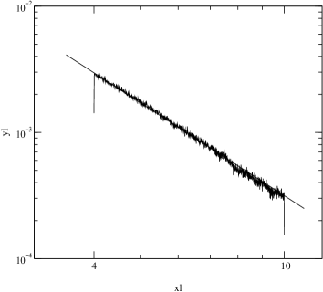
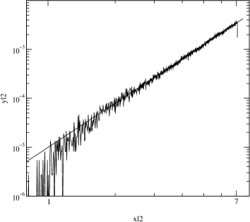
However, both the analytical calculations for the tetrahedron and numerical simulations of larger surfaces indicate that even in the fermionic case the gyration radius distribution has a power–like tail (see the appendix and figure 5 (left)). What is the source of the singular behaviour in this case, when we know that we do not have local spikes? It turns out that there is another type of configuration that can contribute to the tail of the probability distribution $p(R)$ for large $R$. These things look like needles; the four-dimensional degrees of freedom of the co-ordinates in the target space collapse to a one-dimensional, elongated narrow tube.

Figure 4: Snapshots of a susy triangulation from the tail of the gyration radius distribution (right), and a bosonic configuration of comparable size (left). The $x$-component in the plot corresponds to the projection of the vertex position onto the longest principal axis in the system, while the $y$-component describes the distance from the axis. $L$ denotes the length of the tube, $r$ its radius and $R$ the gyration radius

To indentify these configurations we used the principal component analysis (PCA). For each analysed configuration we calculated the correlation matrix $Q_{\mu\nu}=\frac{1}{n}\sum_{i}{X^{\mu}X^{\nu}}$ and its eigenvalues. The eigenvector corresponding to the largest eigenvalue defined the principial axis. For each point on the configuration $X_{i}$ we then calculated its projection on the pricipial axis, $X^{L}_{i}$, and its distance from it, $d_{i}$. We defined the length $L$ and radius $r$ of the tube by

$$L=\max_{i}X^{L}_{i}-\min_{i}X^{L}_{i}\quad\text{and}\quad r=\max_{i}d_{i}$$ (19)

The ratio of length to width can serve as an estimator of the type of the configuration. For the bosonic string, this ratio was $2.26(8)$, and for the fermionic one, $212(20)$. Two typical results of this analysis are depicted in figure 4 where we show, for comparison, snapshots of triangulations for the bosonic (left) and susy (right) models for $n=16$, projected onto the principal axis.

How can the appearance of needles be explained? The bosonic part of the action (8) is a sum of contributions from separate triangles. The contribution from a single triangle is minimal when its three vertices lie on a line, in which case the square of the triangle area is zero. One type of zero-action triangles are the spikes that were discussed in the previous section. On a spike, two vertices of the triangle lie very close to – or, in the limiting case, on top of – each other, so that together with the third vertex they will automatically form a line. Another possible type of zero-action triangles are those that have three distinct (and distant) points that lie on, or close to, a single line. From the point of view of just one triangle, this type of zero-action configuration is more likely to occur than a spiky one, for which one has to move two vertices into exactly the same point; but when one looks at the triangulation as a whole, one sees that the probability for this to happen is actually much smaller, because having three long links means that either there will be three neighbouring triangles with large areas (which is suppressed by the action), or there will be three more triangles lying on exactly the same line. The same argument can then be applied to the neighbours of these triangles as well, and on and on until one arrives at a configuration where all triangles lie on a single line, i.e. a configuration that is just one-dimensional. Contrary to spikes, which are defects that involve only a few triangles and that are basically independent of the rest of the triangulation, a needle requires a global arrangement of vertices that minimizes the action. Such a global arrangement is entropically disfavoured and therefore does not occur in the bosonic model. Here, however, the fermionic determinant provides an additional factor that favours configurations with vertices far removed from each other. As it turns out, this term is sufficient to exceed the damping effect coming from the entropy.

To see this, we will try to estimate the contribution of the needle–like configurations to the partition function. Let us assume that we fix one point on the surface (thus getting rid of the zero mode), and also set the length of one link emerging from this point to $L$. In the following, we will refer to the direction along this link as long and to the transverse directions as short. Consider now a tube of radius $r=1/L$ around the long direction. Clearly, if we constrain all the points to lie inside the tube, the area of each triangle will not exceed $\frac{1}{2}Lr=\frac{1}{2}$. As the action is the sum of the areas squared of the individual triangles, it will be bounded from above by $\frac{1}{4}n_{T}$ independently of $L$. Assuming that all the vertices are free to move independently inside the tube, we can estimate the contribution to the partition function coming from this configuration as :

$$Z_{tube}\sim\int\text{d}L\ L^{3}\left(\text{d}L\ \text{d}r^{3}\right)^{n-2}D(L,r)^{\gamma}.$$ (20)

Here, $D(L,r)$ is the fermionic determinant for the tube–like configuration. We have to integrate over only $n-1$ vertex positions because we already fixed one of them. By choosing a convenient co-ordinate system, we can set this fixed vertex to the origin, and the vertex at the other end of the link to $(L,0,0,0)$. This naturally defines the direction of the needle. Since the needle may point in any direction in four-dimensional space, integration over the position of this point contributes a factor $dLL^{3}$ to the integral. Each of the $n-2$ remaining vertices then contributes one integration over $L$ and three integrations over short components, resulting finally in (20).

The determinant $D(L,r)$ is a uniform polynomial of degree $2(n-1)$, so one would expect at first glance that in the large $L$ limit the leading contribution should be $L^{2(n-1)}$. However, as we will show in the appendix, because of additional symmetries of the matrix all terms containing only long directions cancel, and we get $D(L,r)\sim(r^{2}L^{n-3})^{2}$ for even $n$ and $D(L,r)\sim(r^{4}L^{n-5})^{2}$ for odd $n$. Inserting this into (20) and integrating over all but one long component – which corresponds to substituting $\int dL\rightarrow L$ and $\int dr\rightarrow 1/L$ – we eventually obtain :

$$Z_{tube}\sim dL\ L^{-\alpha}\,,\ \rm{where}\ \left\{\begin{array}[]{ll}\alpha=2n(1-\gamma)+10\gamma-7&\rm{for\ even}\ n\\ &\\ \alpha=2n(1-\gamma)+18\gamma-7&\rm{for\ odd}\ n\end{array}\right.$$ (21)

Because the configuration is essentially one–dimensional and the length of the tube is given by $L$, we expect the gyration radius to be proportional to this, $R\sim L$. Thus, for large $R$, we expect a similarly power–like tail in the gyration radius distribution,

$$\text{d}R\ p(R)\sim\text{d}R\ R^{-\alpha}$$ (22)

if the needle–like configurations dominate in the partition function.

For the purely bosonic case $\gamma=0$, $\alpha=2n-7$ grows with the size of the system and the tail becomes less singular. This suppresses needles. In fact, as we already discussed, in this case the spiky configurations win entropically over the needles, and it is they who are responsible for the singularities of the partition function for bosonic surfaces.

For $\gamma=1$, the formula gives $\alpha=3$ for configurations with an even number of vertices and $\alpha=11$ for those with an odd number. These exponents do not grow with $n$.

For $\gamma>1$, the exponent $\alpha$ decreases with $n$ and very quickly becomes smaller than one. The tail $R^{-\alpha}$ of $p(R)$ becomes non-integrable, signalling that the partition does not exist in this case except for a very few small systems that have $\alpha$ larger than one, such as the tetrahedron, for which the formula predicts $\alpha=1+2\gamma$. (This result for the tetrahedron can actually be derived in a straightforward analytic calculation, as shown in the appendix.)

To test these predictions, we measured the exponent $\alpha$ numerically for different values of $n$ and $\gamma$. Numerical simulations for problems with a power–like distribution are difficult because in this case one has rare but important events. In our case, the distribution $p(R)\sim R^{-\alpha}$ means that we expect rare, long excursions in the configuration space which produce large $R$’s. Technically, it is difficult to explore this part of the phase space, because the bulk of the probability distribution is concentrated around small $R$ where the program spends almost the whole time. To prevent this, we introduced a lower limit $R_{min}$ on $R$, as well as an upper limit $R_{max}$ to prevent the program from doing too long excursions to large values of $R$. Otherwise, the program would not have a well defined autocorrelation time. Experimentally we found it convenient to set the limits $R_{min}=4$ and $R_{max}=10$ when we expected a negative $\alpha$, and only an upper limit $R_{max}=7$ when we expected the distribution $p(R)$ to grow with $R$. In figure 5, we show two examples of the numerically obtained distribution $p(R)$ : for $n=16$ and $\gamma=1$, where according to the formula (21) we expect $\alpha=3$, and for $n=8$ and $\gamma=2$, where we expect $\alpha=-3$. (Note that in the latter case, the partition function would be ill-defined without the upper limit imposed on $R$. We consider it here only for the purpose of testing our formula.)

Figure 5: The distribution $p(R)$ for $n=16$ and $\gamma=1$ (left) and $n=8$ and $\gamma=2$ (right).

The numerical results for $\alpha$ are summarized in table 1.

$\gamma$	$n$	$\alpha_{num}$	$\alpha_{the}$
1	12	2.39(4)	3
1	16	2.41(3)	3
1	7	5.20(1)	11
1	11	3.25(1)	11
2	6	0.92(2)	1
2	8	-3.02(5)	-3
2	10	-7.12(12)	-7

Table 1: Values of the exponent $\alpha$ for various combinations of $n$ and $\gamma$.

We can divide these results into three different cases. For $\gamma=2$, where needles are expected to not just create a tail in the distribution but instead dominate it entirely, the agreement is wonderful, and there is no question that our formula is correct. For $\gamma=1$ and configurations with an even number of vertices, the results are somewhat off, but still in the ballpark of what we expect. One possibility is that this discrepancy is due to finite size effects, and would diminish if we were to go to larger systems; another is that our theoretical argument is simply too rough and works only as a first approximation. In any case, we know from the analysis of sample configurations, as presented in figure 4, that we do have needles in this case. For $\gamma=1$ and an odd number of vertices, the difference is huge but not surprising, since the analysis shows that these configurations are not needles, but look rather like small clumps with a single long spike growing out of them. It would seem that these things are suppressed by a power that is smaller than $-3$ but still larger than $-11$, so that they can dominate over needles in odd-$n$ cases but not in even-$n$ ones.

The estimate of the large $R$ behaviour of the gyration radius distribution for needle-like configurations can easily be extended to the $d=6$ and $d=10$ cases. Since we saw in the four–dimensional case that needles are dominant only for even $n$, we restrict ourselves to these systems. If we repeat the counting of long and short degrees of freedom as in (20), we get with $r\sim 1/L$ :

$$Z_{tube}\sim\int\text{d}L\ L^{d-1}\left(\text{d}L\text{d}r^{(d-1)}\right)^{n-2}D(L,r)^{\gamma}\sim\int\text{d}L\ L^{1+(3-n)(d-2)}D(L,1/L)^{\gamma}$$ (23)

where $D(L,r)$ is now the determinant or the Pfaffian of the Weyl fermion matrix in $d=6$ and $d=10$, respectively. The function $D(L,r)$ is a uniform polynomial of the bosonic components of order $(d-2)(n-1)$ for $d=4,6,10$. Because of zero modes occurring in the minimal blocks of the fermionic matrix (as discussed in detail for $d=4$ in the appendix), the terms with maximal power of $L$ cancel and the leading terms for large $L$ are $\left(r^{2}L^{n-3}\right)^{d-2}$. Thus, for the tube we get $D(L,1/L)\sim L^{(n-5)(d-2)}$. Inserting this into (23) leaves us with

$$Z^{d}_{tube}\sim\int\text{d}L\ L^{1-2(d-2)+(\gamma-1)(n-5)(d-2)}\,.$$ (24)

In the susy case, i. e. $\gamma=1$, the tail of the probability distribution $p(L)\sim L^{1-2(d-2)}$ is independent of $n$. It is the same behaviour as the one obtained in the matrix model from the analysis of the spectrum of large eigenvalues [17].

For $\gamma>1$, the needle-like configurations lead to a non–integrable singularity and the partition function is divergent in this case. For $\gamma=0$, the singularity becomes softer when $n$ goes to infinity. We know, however, that in this case needles do not play any important role in the picture.

To summarize, the discussion presented above allows predictions for the singular behaviour of the partition function in those cases when needle–like configurations dominate in the ensemble.

Discussion

We have investigated geometrical properties of the large $N$ limit of the IKKT matrix model, which corresponds also to the reduced supersymmetric Yang-Mills theory [19]. We showed that the originally four-dimensional theory reduces to a one-dimensional one and is dominated by elongated tube-like configurations. The gyration radius distribution has a power–like tail $p(R)\sim R^{-\alpha}$, where $\alpha$ is roughly consistent with the value of $3$ obtained from the theoretical power–counting for needle-like configurations. Repeated in $d=6,10$ the power–counting for such one–dimensional configurations gives distributions $p(R)\sim R^{-7}$ and $p(R)\sim R^{-15}$, respectively. Strikingly, the same behaviour is expected from the analysis of the large $R$ singularities of the matrix model Yang-Mills integrals [17]. This result has never been proven for the matrix model (except for $N=2$), but if it holds, in view of our geometrical picture it would mean that the Yang–Mills integrals are also dominated by one–dimensional structures for large $R$.

It is clear from our considerations that if too many fermionic degrees of freedom were added to the model ($\gamma>1$), the power $\alpha$ would decrease with $n$ and the partition function would soon become divergent. On the other hand, if there were too few degrees of freedom, as in the purely bosonic case, the singularity of the needle–like configurations would become softer for larger $n$ similarly as in the purely bosonic matrix model [20]. We know, however, that in this case the surface model has a different type of singularity, corresponding to the local creation of spikes, caused by a sort of local flat direction in the action. The effect introduces a stronger singularity that, again, makes the partition function ill-defined. In summary, only the proper susy balance between fermionic and bosonic degrees of freedom guarantees the existence of the surface theory.

The results presented in this work are based on numerical simulations of rather small systems. It would be very interesting to perform a systematic analysis of the finite size effects. This would, however, require a considerable effort to improve the fermionic algorithm.

Appendix

In the first part of the appendix, we will shortly repeat calculations of the partition function $z_{4}(\gamma)$ for the tetrahedron [15], and extend them to calculate the probability distribution of the link length.

Introduce a co-ordinate system in the target space such that the origin coincides with one of these vertices, setting e. g. $X_{4}=(0,0,0,0)$. Next, choose the four axes – called here $L,x,y,$ and $z$ – such that one other vertex lies on the $L$ axis, one lies in the $(L,x)$ plane, and one in the $(L,x,y)$ hyperplane. Thus, we have $X_{1}=(L_{1},0,0,0)$, $X_{2}=(L_{2},x_{2},0,0)$, and $X_{3}=(L_{3},x_{3},y_{3},0)$.

The determinant $D(X)$ in this co-ordinate system becomes [15]

$$D(X)=L_{1}^{2}\ x_{2}^{2}\ y_{3}^{2}$$ (25)

Inserting this into (16) and integrating out all co-ordinates except $L_{1}$ and $x_{2}$ leads to

$$z_{4}(\gamma)=\int_{0}^{\infty}dL_{1}\int_{0}^{\infty}dx_{2}\left(\frac{L_{1}^{4}x_{2}^{3}}{\sqrt{\frac{3}{4}L_{1}^{2}+x_{2}^{2}}^{3}}\right)^{\gamma}e^{-\frac{4}{3}L_{1}^{2}x_{2}^{2}}$$ (26)

For large $L_{1}$, $x_{2}$ is of order $1/L_{1}$, fixed by the combination $L_{1}^{2}x_{2}^{2}$ in the exponent. The integration over $x_{2}$ therefore effectively corresponds to setting $x_{2}\sim L_{1}^{-1}$ (including in the measure $dx_{2}$). Thus, for large $L_{1}$, the resulting integral is dominated by the contribution

$$z_{4}(\gamma)=\int_{0}^{\infty}dL_{1}\ p(L_{1})\sim\int_{0}^{\infty}dL_{1}\ L_{1}^{-1-2\gamma}$$ (27)

The component $L_{1}$ of the vertex $X_{1}$ is the length $L$ of the link between vertices $1$ and $4$. Since there is nothing to distinguish between different links, $p(L)\sim L^{-1-2\gamma}$ can be viewed as the probability distribution of the link length for large $L$.

As can be seen from (25), for the tetrahedron the determinant contains short components to the fourth power, namely $x_{2}^{2}y_{3}^{2}$. We will show that this feature of the determinant is not particular to the tetrahedron, but appears in any needle-like configuration with an even number of vertices, whereas for any needle with an odd number of vertices we find eight short components. The reason for this lies in the Dirac structure of the fermionic matrix.

To see this, let us define a matrix

$$A^{\prime}=A^{\prime}_{0}-i\epsilon A^{\prime}_{1}=\left(\begin{array}[]{cc}{f^{\prime}}^{0}&0\\ 0&{f^{\prime}}^{0}\end{array}\right)-i\epsilon\left(\begin{array}[]{cc}{f^{\prime}}^{3}&{f^{\prime}}^{1}+i{f^{\prime}}^{2}\\ {f^{\prime}}^{1}-i{f^{\prime}}^{2}&-{f^{\prime}}^{3}\end{array}\right)$$ (28)

which for $\epsilon=1$ is equal to the fermionic matrix, $A^{\prime}=-a^{\prime}$. The matrices ${f^{\prime}}^{\mu}$ are antisymmetric $(n-1)\times(n-1)$ matrices, ${f^{\prime}}^{\mu}=-({f^{\prime}}^{\mu})^{T}$. By construction, for needle–like configurations all elements of ${f^{\prime}}^{0}$ are linear in the long components $L$, while those of the ${f^{\prime}}^{k}$ are linear in the short ones, $r_{k}$. Our aim is to prove that the leading term of the determinant $\det A^{\prime}$ is proportional to at least $\epsilon^{4}$ for even configurations and $\epsilon^{8}$ for odd, which is equivalent to saying that the leading term contains at least four/eight small components, which in turn gives $D(L,r)\sim r^{4}L^{2n-6}$ and $D(L,r)\sim r^{8}L^{2n-10}$ for even and odd configurations, respectively. We will use first order perturbation theory to show this.

First of all, note that ${f^{\prime}}^{0}$ has at least one zero eigenvalue, because for strictly one-dimensional configurations with $X_{i}=(X_{i}^{0},0,0,0)$ the action (7) has an additional zero mode coming from invariance under a change $\psi_{i}\rightarrow\psi_{i}+\epsilon X_{i}^{0}$. (This is a discrete remnant of a more general invariance $\psi(\xi)\rightarrow\psi(\xi)+\epsilon g(X^{0}(\xi))$ of the continuous action, with an arbitrary function $g(X^{0})$.) For the truncated matrix ${f^{\prime}}^{0}$, this corresponds to a zero eigenvector

$$w_{i}=X^{0}_{i}-X^{0}_{n}\quad i=1,\dots,n-1$$ (29)

Thus, we also have $\det A^{\prime}_{0}=(\det{f^{\prime}}^{0})^{2}=0$, which already excludes terms of order $\epsilon^{0}$.

Consider now separately the case of even $n$. Because ${f^{\prime}}^{0}$ has the zero eigenvector $w$, $A^{\prime}_{0}$ has at least two eigenvectors $u$ and $d$, which we can write as

$$u=\left(\begin{array}[]{c}w\\ 0\end{array}\right)\quad,\qquad d=\left(\begin{array}[]{c}0\\ w\end{array}\right)\quad$$ (30)

Under a small perturbation $-i\epsilon A^{\prime}_{1}$ the eigenvalues $\lambda$ of $A^{\prime}_{0}$ are changed to $(\lambda-i\epsilon\Delta,\lambda+i\epsilon\Delta^{*})$. Denote the first order correction to $\lambda=0$ by $\Delta_{0}$. The determinant to this order is then proportional to $\epsilon^{2}\Delta_{0}\Delta_{0}^{*}\prod^{\prime}\lambda^{2}$, where the product runs over nonzero eigenvalues of $f^{0}$. $\Delta_{0}$ fulfills the equation

$$\det\left(\begin{array}[]{cc}u^{T}A^{\prime}_{1}u-\Delta_{0}&u^{T}A^{\prime}_{1}d\\ d^{T}A^{\prime}_{1}u&d^{T}A^{\prime}_{1}d-\Delta_{0}\end{array}\right)\ =\ 0$$ (31)

which gives $\Delta_{0}=0$ due to the antisymmetry of the ${f^{\prime}}^{k}$ : $w^{T}{f^{\prime}}^{k}w=0$ for any $k$. Thus, the eigenvalue $\lambda=0$ remains intact to first order, which means that all terms of order $\epsilon^{2}$ likewise vanish in the determinant of $A^{\prime}$. Therefore, the leading terms must be at least of order $\epsilon^{4}$. One can check that, generically, they are indeed of this order.

For odd $n$, ${f^{\prime}}^{0}$ is an even by even antisymmetric matrix and, as such, cannot have just one zero eigenvector but must have at least two, which we will call $v$ and $w$. This in turn means that $A^{\prime}_{0}$ has at least four such eigenvectors, which we write as

$$u_{1}=\left(\begin{array}[]{c}v\\ 0\end{array}\right)\ ,\ u_{2}=\left(\begin{array}[]{c}w\\ 0\end{array}\right)\ ,\ d_{1}=\left(\begin{array}[]{c}0\\ v\end{array}\right)\ ,\ d_{2}=\left(\begin{array}[]{c}0\\ w\end{array}\right)$$ (32)

Repeating the perturbation analysis in $\epsilon$ for the matrix $A^{\prime}$ (28), we find for the first order correction $\Delta_{0}$ :

$$\left[\Delta_{0}^{2}+\sum_{i=1}^{3}\left(v^{T}{f^{\prime}}^{i}w\right)^{2}\right]^{2}=0\,.$$ (33)

We will now argue that all three terms in the sum vanish, and therefore $\Delta_{0}=0$. This follows from the peculiar structure of the matrices ${f^{\prime}}^{\mu}$. As we know, their elements are linear in the components $X^{\mu}$, and moreover all the matrices have the same structure. Therefore, we can introduce a linear function ${f^{\prime}}$ such that ${f^{\prime}}^{\mu}=f(X^{\mu})$. Also, the eigenvector $w$ is likewise linear in $X^{\mu}$, and we can again write $w^{\mu}=w(X^{\mu})$. Now we have

$$v^{T}{f^{\prime}}^{i}w = v^{T}(X^{0})\,{f^{\prime}}(X^{i})\,w(X^{0})$$ (34)

$$= v^{T}(X^{0})\,{f^{\prime}}(X^{i})\,\Big{(}w(X^{0})+w(X^{i})\Big{)}$$

$$= v^{T}(X^{0})\,\Big{(}{f^{\prime}}(X^{0})+{f^{\prime}}(X^{i})\Big{)}\,\Big{(}w(X^{0})+w(X^{i})\Big{)}$$

$$= v^{T}(X^{0})\,{f^{\prime}}(X^{0}+X^{i})\,w(X^{0}+X^{i})$$

$$= 0$$

(In the first step, we just added $v^{T}{f^{\prime}}(X^{i})\,w(X^{i})=0$; in the second, we used the fact that $v^{T}(X_{0})\,{f^{\prime}}(X_{0})=0$; and in the third, we used the linearity of ${f^{\prime}}$ and $w$.)

Thus, we have shown that there are still four zero eigenvalues even to first order of $\epsilon$. As with even $n$, we checked numerically that they are non-zero to the second order. Thus, the leading term in this case behaves as $\epsilon^{8}$.

References

-
[1]
A.M. Polyakov, Phys.Lett. B103 (1981) 207 ;
A.M. Polyakov, Phys. Lett. B103 (1981) 211 ;
A.M. Polyakov, Gauge Fields and Strings, Harwood Academic Publishers 1987 . -
[2]
V. Knizhnik, A. Polyakov and A. Zamolodchikov, Mod. Phys. Lett. A3 (1988) 819 ;
F. David, Mod. Phys. Lett. A3 (1988) 1651 ;
J. Distler and H. Kawai, Nucl. Phys. B321 (1989) 509 . -
[3]
M.B. Green, J.H. Schwarz and E. Witten, Superstring theory, Cambridge University Press 1987 ;
J.G. Polchinsky, String Theory, Cambridge University Press 1998 . -
[4]
F. David, Nucl. Phys. B257 (1985) 45 ;
F. David, Nucl. Phys. B257 (1985) 543 ;
V.A. Kazakov, I. Kostov and A.A. Migdal, Phys. Lett. B157 (1985) 295 ;
V.A. Kazakov, Phys. Lett. A119 (1986) 140 ;
I.K. Kostov, Mod.Phys.Lett. A4 (1989) 217 . -
[5]
E. Brezin and V.A. Kazakov, Phys. Lett. B236 (1990) 144 ;
M. Douglas and S. Shenker, Nucl. Phys. B335 (1990) 635 ;
D. Gross and A.A. Migdal, Phys. Rev. Lett. 64 (1990) 127 . - [6] A.M. Polyakov, Int. J. Mod. Phys. A14 (1999) 645 .
[7]
A. Krzywicki, Phys. Rev. D41 (1990) 3086 ;
F. David, Nucl. Phys. B368 (1992) 671 . -
[8]
F.L. Golterman and D.N. Petcher, Nucl. Phys. B319 (1989) 307 ;
W. Bietenholz, Mod. Phys. Lett. A14 (1999) 51 . - [9] Z. Burda, J. Jurkiewicz and A. Krzywicki, Phys. Rev. D60 (1999) 105029 .
- [10] P.B. Wiegmann, Nucl. Phys. B323 (1989) 330.
- [11] J. Ambjørn, A. Irbäck, J. Jurkiewicz and B. Petersson, Nucl. Phys. B393 (1993) 571 .
[12]
A. Mikovic and W. Siegel, Phys. Lett. B240 (1990) 363 ;
J. Ambjørn and S. Varsted, Phys. Lett. B257 (1991) 305 . -
[13]
N. Ishibashi, H. Kawai, Y. Kitazawa and A. Tsuchiya, Nucl. Phys. B498 (1997) 467 ;
H. Aoki, S. Iso, H. Kawai, Y. Kitazawa and A. Tada, Prog. Theor. Phys. 99 (1998) 713 .
H. Aoki, S. Iso, H. Kawai, Y. Kitazawa, T. Tada, A. Tsuchiya,
Prog. Theor. Phys. Suppl. 134 (1999) 47. -
[14]
I. Bars, Phys. Lett. B245 (1990) 35;
M. Fukuma, H. Kawai, Y. Kitazawa and A. Tsuchiya, Nucl. Phys. B510 (1998) 158. -
[15]
S. Oda and T. Yukawa, Prog. Theor. Phys. 102 (1999) 215 ;
S. Oda and T. Yukawa, Nucl. Phys. B83-84 (2000) 754. -
[16]
W. Krauth, H. Nicolai and M. Staudacher, Phys.Lett. B431 (1998) 31;
J. Nishimura and G. Vernizzi, JHEP 04 (2000) 015.
J. Ambjørn, K.N. Anagnostopoulos, W. Bietenholz, T. Hotta and J. Nishimura, JHEP 07 (2000) 011;
J. Ambjørn, K.N. Anagnostopoulos, W. Bietenholz, T. Hotta and J. Nishimura, JHEP 07 (2000) 013. - [17] W. Krauth and M. Staudacher, Phys. Lett. B 453 (1999) 253.
- [18] J. Ambjørn, B. Durhuus and J. Fröhlich, Nucl. Phys. B257 [FS14] (1985) 433 .
- [19] T. Equichi and H. Kawai, Phys. Rev. Lett. 48 (1982) 1063.
- [20] T. Hotta, J. Nishimura and A. Tsuchiya, Nucl. Phys. B545 (1999) 543.