Abstract

The renormalization of the most general dimension-six four-fermion operators without power subtractions is studied at one loop in lattice perturbation theory using overlap fermions. As expected, operators with different chirality do not mix among themselves and parity-conserving and parity-violating multiplets renormalize in the same way. The renormalization constants of unimproved and improved operators are also the same. These mixing factors are necessary to determine physical matrix elements relevant to many phenomenological applications of weak interactions. The most important are the $K^{0}-\bar{K}^{0}$ and $B^{0}-\bar{B}^{0}$ mixings in the Standard Model and beyond, the $\Delta I=1/2$ rule and $\epsilon^{\prime}/\epsilon$.

1 Introduction

Since the original proposals of using lattice QCD to study hadronic weak decays [1], substantial theoretical and numerical progress has been made. In the most popular lattice regularizations, i.e. Wilson and staggered fermions, the main theoretical aspects of the renormalization of composite four-fermion operators are fully understood [2, 3]. The calculations of the matrix elements relevant for the $K^{0}$–$\bar{K}^{0}$ and $B^{0}$–$\bar{B}^{0}$ mixings have reached a level of accuracy which is unmatched by any other approach [4, 5]; increasing precision has also been achieved in determining the electro-weak penguin amplitudes necessary for the prediction of the CP-violation parameter $\epsilon^{\prime}/\epsilon$ [6]-[12]. Finally, matrix elements of $\Delta S=2$ operators, relevant to the study of FCNC effects in several extensions of the Standard Model (supersymmetry, left-right symmetric models, multi-Higgs models etc.), have also been computed [11]-[13]. Some of these lattice predictions have been fundamental in constraining the parameters of the CKM matrix in the Standard Model (SM) [14, 15] and beyond [16].
Nevertheless, some fundamental phenomena, such as the $\Delta I=1/2$ rule in non-leptonic kaon decays, and the value of $\epsilon^{\prime}/\epsilon$, which measures the direct CP violation in kaon decays, are far from being understood. In the Standard Model these effects can be explained only if the non-perturbative physics gives contributions to matrix elements definitively larger than their factorized values [15]. Therefore a non-perturbative determination of the relevant matrix elements is crucial for predicting these quantities. Lattice QCD is the only method which can address these problems from first principles. Techniques have been developed for both Wilson and staggered fermions, but these methods have not yet produced useful results [6, 17].
To compute non-leptonic weak matrix elements it is essential to construct renormalized operators in definite chiral representations. In the Wilson or SW-Clover lattice regularizations, bare operators do not have a definite chiral behavior due to the presence of the symmetry breaking term in the action. Renormalized operators with the correct chiral properties are recovered as linear combinations of operators with different chirality. The Standard Model $O^{\Delta S=2}$ operator is the most popular example: its matrix element between pseudoscalar states should vanish as $M_{\pi}^{2}$ in the limit $M_{\pi}\rightarrow 0$, while the matrix elements of the wrong-chirality operators which mix with it are expected to go to a constant (and in fact in the kaon mass region they are 2 to 10 times larger than the SM one). Therefore the correct chiral behavior of $O^{\Delta S=2}$ is recovered only if the finite mixing constants are known with high precision. This has been a long-standing problem and has only been solved using Non-Perturbative (NP) renormalization techniques [9, 10, 18]. The situation becomes even worse when the lack of chiral symmetry complicates mixings with lower dimensional operators. This is one of the obstacles to a reliable computation of the matrix elements relevant for $\Delta I=1/2$ and $\epsilon^{\prime}/\epsilon$. On the other hand, with staggered fermions chiral symmetry is preserved, but solving the doubling problem and defining operators with the correct flavor and spin quantum numbers is far from trivial.

Only recently has it been understood [19]-[23] that chiral and flavor symmetries can be preserved simultaneously on the lattice, without fermion doubling, if the fermionic operator $D$ satisfies the Ginsparg-Wilson Relation (GWR) [24]:

$$\gamma_{5}D+D\gamma_{5}=\frac{a}{\rho}D\gamma_{5}D\;.$$ (1)

The GWR implies an exact symmetry of the fermion action at non zero-lattice spacing, which may be regarded as a lattice form of the standard chiral rotation [23]. Nevertheless, it is important to stress that locality, the absence of doubler modes and the correct classical continuum limit are not guaranteed by the GWR in eq. (1). Indeed, there exist lattice fermion actions which satisfy the GWR but which do not meet the above requirements [25]. A breakthrough in this field was achieved through the domain-wall formulation of lattice fermions [26] and by Neuberger through the overlap formulation [21]. He found a solution of the GWR which satisfies all the above requirements and is local [27]:

$$D_{N} = \frac{\rho}{a}\left(1+X\frac{1}{\sqrt{X^{\dagger}X}}\right)$$

$$X = D_{W}-\frac{1}{a}\rho\;,$$ (2)

where $D_{W}$ is the Wilson-Dirac operator and $0<\rho<2r$ (see below). A further remarkable property of Ginsparg-Wilson fermions is the absence of $O(a)$ discretization errors in the action and therefore in the spectrum of the theory. Nevertheless, the local fermionic operators have to be improved to remove the $O(a)$ effects in matrix elements. This step is greatly simplified by the Ginsparg-Wilson relation, as it allows the construction of $O(a)$-improved operators to all orders in $g^{2}$ [28], which renormalize with the same renormalization factors of the unimproved ones. On the other hand, the complicated form of the Neuberger operator in eq. (1) renders its numerical implementation quite demanding for the present generation of computers. However, some progress has been achieved [29] and Monte Carlo simulations seem to be already feasible, at least in the quenched approximation.

Once the action satisfies the GWR and all the properties described above, the quark masses renormalize only multiplicatively and mixings of operators with different chirality are forbidden even at finite cut-off [22]. The most general set of dimension-six four-fermion operators without power subtractions is

$$O_{\Gamma_{A}\Gamma_{B}} = \bar{\psi}_{1}\Gamma^{l}_{A}\psi_{2}\cdot\bar{\psi}_{3}\Gamma^{l}_{B}\psi_{4}$$ (3)

$$O^{F}_{\Gamma_{A}\Gamma_{B}} = \bar{\psi}_{1}\Gamma^{l}_{A}\psi_{4}\cdot\bar{\psi}_{3}\Gamma^{l}_{B}\psi_{2}\;.$$

The main result of this paper is the evaluation of the mixing pattern of these operators at one loop in perturbation theory in the overlap lattice regularization: we compute their renormalization constants and we show how the Neuberger action greatly simplifies the mixing among them.

The renormalization constants are necessary for extracting physical matrix elements from numerical simulations. The matrix elements of the operators studied in this work are relevant in many phenomenological applications of weak interactions. They are necessary for predicting the $K^{0}-\bar{K}^{0}$ and $B^{0}-\bar{B}^{0}$ mixing amplitudes in the Standard Model and in several extensions of it (supersymmetry, left-right symmetric models, multi-Higgs models etc.). By using chiral perturbation theory, they can also be related to the $\Delta I=3/2$ matrix elements relevant for the prediction of $\epsilon^{\prime}/\epsilon$. They are also necessary for estimating the $B^{0}_{s}-\bar{B}^{0}_{s}$ width difference and the $O(1/m_{b}^{3})$ corrections in inclusive b-hadron decay rates [30]. The renormalization constants we have computed are also relevant for the study of the $\Delta I=1/2$ rule and $\epsilon^{\prime}/\epsilon$ on the lattice. The operators involved in these computations can mix with same- as well as lower-dimension operators. The key observation in these cases [31] is that the lower-dimension operators do not change the anomalous dimensions of the original operators. Therefore the mixings among dimension-six operators can be obtained from those of the operators studied in this paper.

Perturbative computations with the overlap-Dirac operator are much more cumbersome than for Wilson fermions, due to the complicated structure of the vertices in the action (see Appendix A). For this reason it is very useful to use an intermediate renormalization scheme to separate as much as possible the computations performed using lattice perturbation theory (where, for example, the Fierz rearrangements work) from the continuum perturbation theory which is much simpler. The RI renormalization scheme proposed in [32, 33] is the optimum choice: we first renormalize lattice operators in the RI scheme using only lattice perturbation theory and then the matching with one of the $\overline{\mbox{MS}}$ schemes is done in continuum perturbation theory. Lattice and continuum regularizations are used independently taking full advantage of their properties.
In Ref. [34], renormalization constants of local bilinear fermion operators have been computed in the $\overline{\mbox{MS}}$ renormalization scheme using the lattice overlap regularization. We computed these renormalization constants in the RI scheme, matched them in $\overline{\mbox{MS}}$ and verified that our results are in agreement with those of Ref. [34]. Then we computed the renormalization constants of the four-fermion operators we are interested in following two independent ways: the direct computation, like in Ref. [35], and one which uses the Fierz and charge conjugation rearrangements to compute the four-fermion Green’s functions in terms of the bilinear ones [36, 8]. The agreement of the results is also a non-trivial check that the numerical integrals with the Neuberger propagators and vertices are well estimated.

A further determination of the renormalization constants considered in this paper can be obtained using numerical NP methods such as those in Refs. [33, 39], applied to Neuberger fermions. However, perturbative estimates are very useful because often they are very good approximations and they furnish a consistency check of the NP methods. Moreover, for Neuberger fermions the perturbative computations can remain the only determinations of the renormalization constants for some time.

The paper is organized as follows: in section 2 we define the overlap fermion action used; in section 3 we discuss the bilinear renormalization constants; in section 4 we address the mixing of the four-fermion operators and report the results for the renormalization constants; in section 5 we state our conclusions.

2 Basic definitions

The QCD lattice regularization we consider for massless fermions is described by the action

$$S_{L}=\frac{6}{g_{0}^{2}}\sum_{P}\bigg{[}1-\frac{1}{6}\mbox{Tr}\;\bigl{[}U_{P}+U_{P}^{\dagger}\bigr{]}\bigg{]}+\sum_{i=1}^{N_{f}}\sum_{x,y}\bar{\psi}_{i}(x)\,D_{N}(x,y)\,\psi_{i}(y),$$ (4)

where, in standard notation, $U_{P}$ is the Wilson plaquette and $g_{0}$ the bare coupling constant. $D_{N}$ is the Neuberger-Dirac operator defined in eq. (1), where the massless Wilson operator $D_{W}$ is defined as

$$D_{W}=\frac{1}{2}\gamma_{\mu}(\nabla_{\mu}+\nabla^{*}_{\mu})-\frac{r}{2}a\nabla^{*}_{\mu}\nabla_{\mu}$$ (5)

and $\nabla_{\mu}$ and $\nabla^{*}_{\mu}$ are the forward and backward lattice derivatives, i.e.

$$\nabla_{\mu}\psi(x) = \frac{1}{a}\Big{[}U_{\mu}(x)\psi(x+a\hat{\mu})-\psi(x)\Big{]}$$

$$\nabla_{\mu}^{*}\psi(x) = \frac{1}{a}\Big{[}\psi(x)-U^{\dagger}_{\mu}(x-a\hat{\mu})\psi(x-a\hat{\mu})\Big{]}\;.$$ (6)

The range of the Wilson parameter is $0<r<1$ and $U_{\mu}(x)$ is the lattice gauge link. Eq. (1) implies a continuous symmetry of the fermion action in (4), which may interpreted as a lattice form of chiral symmetry [23]:

$$\delta\psi=\gamma_{5}\left(1-\frac{1}{2\rho}aD_{N}\right)\psi,\qquad\delta\bar{\psi}=\bar{\psi}\left(1-\frac{1}{2\rho}aD_{N}\right)\gamma_{5}.$$ (7)

The corresponding flavor non-singlet chiral transformations are defined including a color group generator in eq. (7). The generalization to massive fermions is simple [40]: in eq. (4) $D_{N}$ has to be replaced by

$$D_{N}\longrightarrow\left(1-\frac{1}{2\rho}am^{i}_{0}\right)D_{N}+m^{i}_{0}$$ (8)

where $m^{i}_{0}$ is the bare physical quark mass of flavor $i$. The Feynman rules of the action defined in Eq. (4) are given in Appendix A and are in agreement with those used by [34, 41, 42]. Throughout this paper we will use only mass independent renormalization schemes (RI and $\overline{\mbox{MS}}$) and therefore all our computations are performed with massless quarks.

3 Renormalization of Bilinear Operators

In this section we set our notation for bilinear operators and we report the results we have obtained for their renormalization constants in the RI and $\overline{\mbox{MS}}$ schemes.
A generic non-singlet quark bilinear is defined as

$$O_{\Gamma}(x)=\bar{\psi}_{1}(x)\Gamma\psi_{2}(x)$$ (9)

where the flavors $\psi_{1}-\psi_{2}$ are different and $\Gamma$ is a generic Dirac matrix. The GWR ensures that no lattice artifacts of $O(a)$ are present in the action and therefore also not in the spectrum of the theory. However, matrix elements of operators are still affected by $O(a)$ discretization errors that have to be removed by improving the fermionic operators. In Refs. [28] it is shown that, for massless quarks, the improved bilinear operator is given by

$$O_{\Gamma}^{I}=\bar{\psi}\Big{(}1-\frac{1}{2\rho}aD_{N}\Big{)}\,\Gamma\,\Big{(}1-\frac{1}{2\rho}aD_{N}\Big{)}\psi\;\;.$$ (10)

It can be proven [34, 28] that the renormalization constants of $O_{\Gamma}^{I}$ are the same as those of the corresponding $O_{\Gamma}$. Therefore all the results obtained in this section for local bilinear operators also remain valid for the corresponding improved operators.
The renormalized bilinear operators are defined by

$$\widehat{O}_{\Gamma}(\mu)=Z_{\Gamma}(a\mu)O_{\Gamma}(a)\;$$ (11)

and the chiral symmetry in eq. (7) imposes the constraints

$$Z_{A} = Z_{V}$$

$$Z_{P} = Z_{S}\;$$ (12)

on the renormalization constants.

The quark propagator in momentum space is denoted by $S(p)$ (for the conventions adopted throughout the paper see Appendix B). The two-point fermionic Green’s function of a bilinear inserted at the origin ($x=0$) is

$$G_{\Gamma}(x_{1},x_{2})=\langle\psi_{1}(x_{1})O_{\Gamma}(0)\bar{\psi}_{2}(x_{2})\rangle\;,$$ (13)

its Fourier transform with equal external momenta is

$$G_{\Gamma}(p)=\int dx_{1}dx_{2}e^{-ip(x_{1}-x_{2})}G_{\Gamma}(x_{1},x_{2})\;,$$ (14)

and the corresponding amputated correlation function is defined as

$$\Lambda_{\Gamma}(p)=S^{-1}(p)G_{\Gamma}(p)S^{-1}(p)\;.$$ (15)

The renormalized quark propagator is

$$\widehat{S}(p,\mu)=Z_{\psi}(a\mu)S(p,a)\;,$$ (16)

where $Z_{\psi}^{1/2}$ is the quark field renormalization constant, and the renormalized Green’s functions are

$$\widehat{G}_{\Gamma}(p,\mu) = Z_{\psi}(\mu a)Z_{\Gamma}(\mu a)G_{\Gamma}(p,a)\;,$$ (17)

$$\widehat{\Lambda}_{\Gamma}(p,\mu) = Z^{-1}_{\psi}(\mu a)Z_{\Gamma}(\mu a)\Lambda_{\Gamma}(p,a)\;.$$ (18)

The anomalous dimensions of composite operators are defined as

$$\gamma_{\Gamma}(\alpha_{s})=-2Z_{\Gamma}^{-1}\mu^{2}\frac{d}{d\mu^{2}}Z_{\Gamma}=\sum_{i=0}^{\infty}\gamma_{\Gamma}^{(i)}\left(\frac{\alpha_{s}}{4\pi}\right)^{i+1}\;,$$ (19)

where $\alpha_{s}=g^{2}/4\pi$ is the strong coupling constant. If a renormalization scheme which preserves the chiral Ward Identities (WI) is chosen (such as $\overline{\mbox{MS}}$ or RI), then

$$\gamma_{A}=\gamma_{V}=0\;,$$ (20)

$$\gamma_{P}=\gamma_{S}=-\gamma_{m}\;,$$

where $\gamma_{m}$ is the anomalous dimension of the quark mass. Moreover the $\gamma_{\Gamma}^{(0)}$s are renormalization-scheme independent and gauge invariant and their values are reported in Table 1.
The anomalous dimensions are properties of the renormalized operators: they are independent of the regularization scheme adopted and depend only on the renormalization conditions imposed (the renormalization scheme) and the renormalized coupling constant used. For a given operator, defining the renormalization conditions is equivalent to fixing $\gamma_{\Gamma}(\alpha_{s})$, i.e. $\gamma_{\Gamma}(\alpha_{s})$ uniquely determines the scheme in a regularization invariant way. Therefore, $\gamma_{\Gamma}$ can be computed in a simpler regularization, like Naive Dimensional Regularization (NDR), provided that the renormalization conditions are the same. The evolution of the renormalized operators is determined by solving the Renormalization Group Equations and, in a given scheme, is

$$\widehat{O}_{\Gamma}(\mu)=\frac{c_{\Gamma}(\mu)}{c_{\Gamma}(\mu_{0})}O_{\Gamma}(\mu_{0})\;,$$ (21)

where $c_{\Gamma}(\mu)$ at Next-to-Leading Order (NLO)

$$c_{\Gamma}(\mu)=\left(\alpha_{s}(\mu)\right)^{\gamma_{\Gamma}^{(0)}/(2\beta_{0})}\left[1+\frac{\alpha_{s}(\mu)}{4\pi}\left(\frac{\gamma^{(1)}_{\Gamma}}{2\beta_{0}}-\frac{\beta_{1}\gamma^{(0)}_{\Gamma}}{2\beta_{0}^{2}}\right)\right]$$ (22)

is scheme dependent. In eq. (22) $\beta_{0}$ and $\beta_{1}$ are the first two coefficients of the $\beta$ function of QCD. For $\gamma_{\Gamma}^{(1)}$ in RI or $\overline{\mbox{MS}}$ see for example [43]. The Renormalization Group Invariant (RGI) operators can be defined as [43]-[45]

$$\widehat{O}_{\Gamma}^{\mbox{\scriptsize RGI}}=\frac{1}{c_{\Gamma}(\mu)}\widehat{O}_{\Gamma}(\mu)=Z^{\mbox{\scriptsize RGI}}_{\Gamma}(a)O_{\Gamma}(a)\;,$$ (23)

where

$$Z^{\mbox{\scriptsize RGI}}_{\Gamma}(a)=\frac{Z_{\Gamma}(\mu a)}{c_{\Gamma}(\mu)}\;.$$ (24)

$\widehat{O}_{\Gamma}^{\mbox{\scriptsize RGI}}$ is independent of the scheme, scale and gauge chosen to renormalize the operators, while $Z^{\mbox{\scriptsize RGI}}_{\Gamma}(a)$ depends only on the regularization and not on the scheme, scale and gauge.

As discussed in the introduction, it is very helpful to separate computations which can be performed using only lattice perturbation theory from those done in the continuum. In this regard the RI renormalization scheme proposed in [32, 33] is the optimum choice: it preserves all the relevant symmetries (chirality and switch, see below) and it can also be easily implemented non-perturbatively [33]. The matching with a “continuum” renormalization scheme, for example $\overline{\mbox{MS}}$, remains necessary because almost all the Wilson coefficients are computed in the continuum, but it can be done using continuum perturbation theory only. Therefore lattice and continuum regularizations are used independently taking full advantage of their properties. In the following we will indicate the renormalization scheme adopted with a superscript in the renormalization quantities, i.e. $Z_{\Gamma}^{\mbox{\scriptsize RI}}$ and $Z_{\Gamma}^{\overline{\mbox{\scriptsize MS}}}$ for RI and $\overline{\mbox{MS}}$ schemes respectively.

Using the Feynman rules defined in Appendix A, we computed the self energy of the quark propagator and the amputated Green’s functions of bilinear operators between off-shell quark states at one loop in perturbation theory in a generic covariant gauge. The full expressions we obtained are reported in Appendix D and they can be used to impose any renormalization condition in any covariant gauge.

		$\psi$	S	V	T
Continuum PT
$\bar{\gamma}^{(0)}$		0	-6	0	2
$\Delta^{\overline{\mbox{\scriptsize MS}},\mbox{\scriptsize RI}}$		0	-4	0	0
	$\rho$	Lattice PT
	0.2	-235.80762	1.31942	1.52122	1.58848
	0.3	-150.61868	1.89625	1.52277	1.39828
	0.4	-108.19798	2.38060	1.52448	1.23911
	0.5	-82.86081	2.80522	1.52637	1.10009
	0.6	-66.05227	3.18782	1.52845	0.97532
	0.7	-54.10921	3.53927	1.53074	0.86124
	0.8	-45.20179	3.86686	1.53329	0.75543
	0.9	-38.31447	4.17577	1.53611	0.65622
$B$	1.0	-32.83862	4.46989	1.53924	0.56236
	1.1	-28.38734	4.75224	1.54274	0.47290
	1.2	-24.70304	5.02527	1.54665	0.38711
	1.3	-21.60760	5.29104	1.55105	0.30438
	1.4	-18.97397	5.55135	1.55601	0.22422
	1.5	-16.70910	5.80783	1.56163	0.14623
	1.6	-14.74330	6.06201	1.56804	0.07005
	1.7	-13.02336	6.31544	1.57541	-0.00460
	1.8	-11.50798	6.56970	1.58394	-0.07798

Table 1: Perturbative values in the continuum and on the lattice in the Landau gauge, where $\bar{\gamma}^{(0)}=\gamma^{(0)}/C_{F}$ while the $B$s contain the proper vertex contribution only.

The RI scheme is imposed by taking the trace of the amputated Green’s functions in the Landau gauge ($\alpha=0$) [33]. The renormalization constant of the quark field is then defined as

$$Z^{\mbox{\scriptsize RI}}_{\psi}=-i\frac{1}{48}\mbox{Tr}\;\gamma_{\mu}\frac{\partial S^{-1}(p)}{\partial p_{\mu}}\Bigg{|}_{p^{2}=\mu^{2}}\;,$$ (25)

while the renormalization constants of the bilinear operators are given by

$$(Z^{\mbox{\scriptsize RI}}_{\psi}(\mu a))^{-1}Z^{\mbox{\scriptsize RI}}_{\Gamma}(\mu a)\mbox{Tr}\;\Big{[}P_{\Gamma}\Lambda_{\Gamma}(p,a)\Big{]}\Bigg{|}_{p^{2}=\mu^{2}}=1\;,$$ (26)

where the trace is over both color and spin indices and $P_{\Gamma}$ are suitable projectors on the tree-level operators defined in Appendix C. In general, these renormalization conditions differ from the standard MOM perturbative prescriptions (see for example [36]), where the renormalization constants are extracted only from terms proportional to the tree-level matrix elements of the operators under consideration. The differences are evident from the expressions of the quark propagator and the amputated Green’s functions reported in Appendix D. In the standard procedure, finite terms such as $p\!\!\!/\,p_{\mu}/p^{2}$ in the vector current are considered as part of the matrix elements of the operators, whereas with the projectors they give additional finite contributions to the renormalization constants. These terms are the same on the lattice and in the continuum and they cancel when one computes the difference between the continuum and the lattice renormalization constants, as in the standard perturbative procedure.
Using eqs. (25) and (26) and the results reported in Appendix D we obtained

$$Z^{\mbox{\scriptsize RI}}_{\psi} = 1-\frac{g_{0}^{2}}{16\pi^{2}}C_{F}\left[\frac{\bar{\gamma}_{\psi}^{(0)}}{2}\log(\mu a)^{2}+B_{\psi}\right]$$

$$Z^{\mbox{\scriptsize RI}}_{\Gamma} = 1-\frac{g_{0}^{2}}{16\pi^{2}}C_{F}\left[\frac{\bar{\gamma}_{\Gamma}^{(0)}}{2}\log(\mu a)^{2}+B_{\Gamma}+B_{\psi}\right]\;,$$ (27)

where the $\bar{\gamma}_{\Gamma}^{(0)}$ and $B$s are reported in Table 1.
Once the operators have been renormalized in RI, the matching with another given scheme $\chi$ is obtained with

$$Z^{\chi}_{\Gamma}(\mu a)=c^{\chi}_{\Gamma}(\mu)Z^{\mbox{\scriptsize RGI}}_{\Gamma}(a)=\frac{c^{\chi}_{\Gamma}(\mu)}{c^{\mbox{\scriptsize RI}}_{\Gamma}(\mu)}Z^{\mbox{\scriptsize RI}}_{\Gamma}(\mu a)\;,$$ (28)

where the $c^{\mbox{\scriptsize RI}}_{\Gamma}(\mu)$ are reported in [43] for the bilinears, defined with the same conventions adopted in this paper.
To compare our results with [34], we report explicitly the matching coefficients for the $\overline{\mbox{MS}}$ scheme. The chiral WI imply $Z_{V}^{\mbox{\scriptsize RI}}=Z_{V}^{\overline{\mbox{\scriptsize MS}}}$, $Z_{A}^{\mbox{\scriptsize RI}}=Z_{A}^{\overline{\mbox{\scriptsize MS}}}$ and

$$\frac{Z_{S}^{\mbox{\scriptsize RI}}}{Z_{P}^{\mbox{\scriptsize RI}}}=\frac{Z_{S}^{\overline{\mbox{\scriptsize MS}}}}{Z_{P}^{\overline{\mbox{\scriptsize MS}}}}=1\;.$$ (29)

A straightforward computation in NDR gives

$$Z_{\Gamma}^{\overline{\mbox{\scriptsize MS}}}(a\mu)=\left[1-C_{F}{\displaystyle{\alpha_{s}\over 4\pi}}(\Delta^{\overline{\mbox{\scriptsize MS}},\mbox{\scriptsize RI}}_{\Gamma}+\Delta^{\overline{\mbox{\scriptsize MS}},\mbox{\scriptsize RI}}_{\psi})\right]Z_{\Gamma}^{\mbox{\scriptsize RI}}(a\mu),$$ (30)

where the $\Delta^{\overline{\mbox{\scriptsize MS}},\mbox{\scriptsize RI}}$s are reported in Table 1. In the $\overline{\mbox{MS}}$ scheme, the renormalization constants of gauge-invariant operators are independent of the gauge. Therefore, the dependence on the gauge and external states of the RI scheme cancels the corresponding dependence of the matching coefficients. Our results in $\overline{\mbox{MS}}$ are in agreement with those of Ref. [34].

4 Four-fermion operators

In this section we introduce the most general set of dimension-six four-fermion operators we are interested in, we analyze their mixing pattern exploiting only the symmetries of the underlying theory and finally we compute the necessary renormalization constants at 1-loop in perturbation theory. A very exhaustive non-perturbative analysis for Wilson fermions has been done in Ref. [18]. We will proceed on the same lines with the advantage of having the additional chiral symmetry in eq. (7) which forbids mixing among operators which belong to multiplets with different chirality [22].
The generic set of four-fermion operators we are interested in is

$$O_{\Gamma_{A}\Gamma_{B}} = \bar{\psi}_{1}\Gamma^{l}_{A}\psi_{2}\cdot\bar{\psi}_{3}\Gamma^{l}_{B}\psi_{4}$$ (31)

$$O^{F}_{\Gamma_{A}\Gamma_{B}} = \bar{\psi}_{1}\Gamma^{l}_{A}\psi_{4}\cdot\bar{\psi}_{3}\Gamma^{l}_{B}\psi_{2}\;,$$

where the flavors $\psi_{1}-\psi_{4}$ are all different and the $\Gamma^{l}_{A}$ are generic Dirac matrices with $l$ representing the contracted Lorenz indices (if any). The 20 operators in (31) form a complete basis of four-fermion operators. Operators with the color indices contracted in a different way can be expressed as linear combinations of the ones in eq. (31) using the color Fierz identity (63) in Appendix B.
The $O(a)$ discretization errors in on-shell four-fermion matrix elements can be removed by using the improved operator

$$\bar{\psi}\Big{(}1-\frac{1}{2\rho}aD_{N}\Big{)}\,\Gamma_{A}\,\Big{(}1-\frac{1}{2\rho}aD_{N}\Big{)}\psi\cdot\bar{\psi}\Big{(}1-\frac{1}{2\rho}aD_{N}\Big{)}\,\Gamma_{B}\,\Big{(}1-\frac{1}{2\rho}aD_{N}\Big{)}\psi.$$ (32)

This can be proven along the lines used in Refs. [28] for the case of two-quark operators. Here we just sketch the argument, which is valid for any reasonable action which satisfies the GWR. Starting from the Neuberger operator $D_{N}$, one can define the associated operator [25]

$$K_{N}=\Big{(}1-\frac{1}{2\rho}aD_{N}\Big{)}^{-1}D_{N},$$ (33)

which has the same chiral properties as the continuum Dirac operator, i.e. $\{K_{N},\gamma_{5}\}=0$. The propagator $K^{-1}_{N}$ is free of $O(a)$ corrections and, although otherwise not well-behaved and so not useful in practice, it turns out to be very useful for the construction of operators that are improved. In fact, the four-fermion correlation function

$$\Big{\langle}\frac{1}{K_{N}}\Gamma_{A}\frac{1}{K_{N}}\cdot\frac{1}{K_{N}}\Gamma_{B}\frac{1}{K_{N}}\Big{\rangle}=$$ (34)

$$\Big{\langle}\frac{1}{D_{N}}\Big{(}1-\frac{1}{2\rho}aD_{N}\Big{)}\Gamma_{A}\Big{(}1-\frac{1}{2\rho}aD_{N}\Big{)}\frac{1}{D_{N}}\cdot\frac{1}{D_{N}}\Big{(}1-\frac{1}{2\rho}aD_{N}\Big{)}\Gamma_{B}\Big{(}1-\frac{1}{2\rho}aD_{N}\Big{)}\frac{1}{D_{N}}\Big{\rangle}\;$$

is automatically improved. In the last line we have used eq. (33) to re-express the Green’s function in terms of the Neuberger propagator, and from this we can read off the improved operator. Thus, the Ginsparg-Wilson relation highly simplifies the improvement of the four-fermion operators at all orders in perturbation theory. Moreover, the renormalization factors for corresponding improved and unimproved operators are the same. This happens because in 1-loop amplitudes a $D_{N}$ factor can combine with a quark propagator but, since it has an $a$ in front and (contrary to the Wilson case) there is no $1/a$ factor in the propagator, as additive mass renormalization is forbidden by chiral symmetry, its contribution to the renormalization factors is zero [34].

The symmetries relevant for studying the mixing of the operators that we consider are Parity (${\cal P}$), the Switch (${\cal S}$) transformation $\psi_{2}\leftrightarrow\psi_{4}$ and chiral symmetry in eq. (7). They allow splitting the original basis into smaller independent multiplets. For parity-conserving (${\cal P}=1$) operators it is useful to define the following bases

$$Q^{\pm}_{1} = O^{\pm}_{VV}+O^{\pm}_{AA}$$

$$Q^{\pm}_{2} = O^{\pm}_{VV}-O^{\pm}_{AA}$$

$$Q^{\pm}_{3} = O^{\pm}_{SS}-O^{\pm}_{PP}$$

$$Q^{\pm}_{4} = O^{\pm}_{SS}+O^{\pm}_{PP}$$

$$Q^{\pm}_{5} = O^{\pm}_{TT}\;,$$ (35)

and for the parity-violating (${\cal P}=-1$)

$${\cal Q}^{\pm}_{1} = O^{\pm}_{VA}+O^{\pm}_{AV}$$

$${\cal Q}^{\pm}_{2} = O^{\pm}_{VA}-O^{\pm}_{AV}$$

$${\cal Q}^{\pm}_{3} = -O^{\pm}_{SP}+O^{\pm}_{PS}$$

$${\cal Q}^{\pm}_{4} = O^{\pm}_{SP}+O^{\pm}_{PS}$$

$${\cal Q}^{\pm}_{5} = O^{\pm}_{T\widetilde{T}}\;,$$ (36)

where

$$O^{\pm}_{\Gamma_{A}\Gamma_{B}} = \frac{1}{2}\left[O_{\Gamma_{A}\Gamma_{B}}\pm O^{F}_{\Gamma_{A}\Gamma_{B}}\right]\;,$$ (37)

and $\widetilde{T}=\sigma_{\mu\nu}\gamma_{5}$. Since the lattice preserves parity, the two sets of operators (4) and (4) renormalize independently. Using continuous chiral transformations it is easy to show that, at variance with Wilson fermions, they renormalize with the same renormalization matrices [18]. We have explicitly verified this property at one loop in perturbation theory. In the following we will then consider only the parity-conserving operators in eqs. (4). Among them, the five $Q^{+}_{i}$ are left invariant under a switch transformation (${\cal S}=1$), while the $Q^{-}_{i}$ change sign (${\cal S}=-1$). Therefore the two sets renormalize independently as

$$\widehat{Q}^{\pm}_{i}(\mu)=\widehat{Z}^{\pm}_{ij}(\mu a)Q^{\pm}_{j}(a)\;,$$ (38)

where $\widehat{Z}^{\pm}$ are the renormalization constant matrices.
The operators of the bases (4) do not belong, in general, to irreducible representations of the chiral group. Nevertheless chiral symmetry imposes many constraints on the matrix of the renormalization constants when a scheme which preserves it together with the switch symmetry is chosen. The most general mixing matrix under these constraints reads

$$\widehat{Z}^{\pm}=\pmatrix{Z^{\pm}_{11}&0&0&0&0\cr 0&Z_{22}&\pm Z_{23}&0&0\cr 0&\pm Z_{32}&Z_{33}&0&0\cr 0&0&0&Z^{\pm}_{44}&Z^{\pm}_{45}\cr 0&0&0&Z^{\pm}_{54}&Z^{\pm}_{55}\cr}\;.$$ (39)

Note that for $i,j=2,3$, $Z^{+}_{ij}$ and $Z^{-}_{ij}$ are related. Therefore for Neuberger fermions there are only 14 independent renormalization constants, which would instead become 64 if the Wilson action were used. The particular structure of the matrix in eq. (39) also simplifies the implementation of non-perturbative techniques [33, 39].

Analogously to the bilinears, denoting by $x_{1},x_{3}$ and $x_{2},x_{4}$ the coordinates of the outgoing and incoming quarks respectively, the four-point Green’s functions are defined as

$$G^{\pm}_{i}(x_{1},x_{2},x_{3},x_{4})=\langle\psi_{1}(x_{1})\bar{\psi}_{2}(x_{2})Q^{\pm}_{i}(0)\psi_{3}(x_{3})\bar{\psi}_{4}(x_{4})\rangle\,,$$ (40)

where $\langle\cdots\rangle$ denotes the vacuum expectation value. Note that $G^{\pm}_{i}$ depends implicitly on the four color and Dirac indices carried by the external fermion fields. The Fourier transform of the Green’s function (40) at equal external momenta $p$ is defined as

$$G^{\pm}_{i}(p)=\int dx_{1}dx_{2}dx_{3}dx_{4}e^{-ip(x_{1}+x_{3}-x_{2}-x_{4})}G^{\pm}_{i}(x_{1},x_{2},x_{3},x_{4})\;.$$ (41)

The corresponding amputated correlation functions is defined as

$$\Lambda^{\pm}_{i}(p)=S^{-1}(p)S^{-1}(p)G^{\pm}_{i}(p)S^{-1}(p)S^{-1}(p)\;.$$ (42)

From the above definitions we find for the renormalized Green’s functions

$$\widehat{G}^{\pm}_{i}(p) = Z^{2}_{\psi}\widehat{Z}^{\pm}_{ij}G^{\pm}_{j}(p)\;,$$

$$\widehat{\Lambda}^{\pm}_{i}(p) = Z^{-2}_{\psi}\widehat{Z}^{\pm}_{ij}\Lambda^{\pm}_{j}(p)\;.$$ (43)

The anomalous dimension matrices are defined as

$$\widehat{\gamma}^{\pm}(\alpha_{s})\equiv-2(\widehat{Z}^{\pm})^{-1}\mu^{2}\frac{d}{d\mu^{2}}\widehat{Z}^{\pm}=\sum_{i=0}^{\infty}\widehat{\gamma}^{\pm(i)}\left(\frac{\alpha_{s}}{4\pi}\right)^{i+1}\;$$ (44)

and, if the renormalization scheme preserves chiral symmetry, they have the same structure as in eq. (39). At first order in $\alpha_{s}$ we obtain

$$\gamma^{+(0)}_{11}=-\frac{2}{3}\bar{\gamma}^{(0)}_{S} \gamma^{-(0)}_{11}=\frac{4}{3}\bar{\gamma}^{(0)}_{S}$$ (45)

$$\gamma^{(0)}_{22}=-\frac{1}{3}\bar{\gamma}^{(0)}_{S} \gamma^{(0)}_{23}=-2\bar{\gamma}^{(0)}_{S}$$

$$\gamma^{(0)}_{32}=0 \gamma^{(0)}_{33}=\frac{8}{3}\bar{\gamma}^{(0)}_{S}$$

$$\gamma^{+(0)}_{44}=\frac{23\bar{\gamma}^{(0)}_{S}+9\bar{\gamma}^{(0)}_{T}}{12} \gamma^{-(0)}_{44}=\frac{41\bar{\gamma}^{(0)}_{S}-9\bar{\gamma}^{(0)}_{T}}{12}$$

$$\gamma^{+(0)}_{45}=\frac{-\bar{\gamma}^{(0)}_{S}+\bar{\gamma}^{(0)}_{T}}{12} \gamma^{-(0)}_{45}=\frac{5(\bar{\gamma}^{(0)}_{S}-\bar{\gamma}^{(0)}_{T})}{12}$$

$$\gamma^{+(0)}_{54}=\frac{5(\bar{\gamma}^{(0)}_{S}-\bar{\gamma}^{(0)}_{T})}{4} \gamma^{-(0)}_{54}=\frac{-\bar{\gamma}^{(0)}_{S}+\bar{\gamma}^{(0)}_{T}}{4}$$

$$\gamma^{+(0)}_{55}=\frac{-9\bar{\gamma}^{(0)}_{S}+41\bar{\gamma}^{(0)}_{T}}{12} \gamma^{-(0)}_{55}=\frac{9\bar{\gamma}^{(0)}_{S}+23\bar{\gamma}^{(0)}_{T}}{12}\;,$$

which agree with [37, 38], where the anomalous dimension matrices at two loops in the same bases can also be found.
The renormalization group evolution of the four-fermion operators, in a scheme which preserves chiral and the switch symmetry, is

$$\widehat{Q}^{\pm}(\mu)=\widehat{w}^{\pm}(\mu)[\widehat{w}^{\pm}(\mu_{0})]^{-1}\widehat{Q}^{\pm}(\mu_{0})\;,$$ (46)

where in this case $\widehat{w}^{\pm}(\mu)$ are matrices which depend only on the anomalous dimensions and $\alpha_{s}$. Their expression at NLO in a generic scheme can be found in [37, 38, 12]. Analogously to the bilinears, the RGI operators can be defined as [12]

$$[\widehat{Q}^{\pm}]^{\mbox{\scriptsize RGI}}=[\widehat{w}^{\pm}(\mu)]^{-1}\widehat{Q}^{\pm}(\mu)=[\widehat{Z}^{\pm}(a)]^{\mbox{\scriptsize RGI}}Q^{\pm}(a)\;,$$ (47)

where

$$[\widehat{Z}^{\pm}(a)]^{\mbox{\scriptsize RGI}}=[\widehat{w}^{\pm}(\mu)]^{-1}\widehat{Z}^{\pm}(\mu a)\;.$$ (48)

As for the scheme, scale and gauge dependences, these definitions have the same properties as for bilinears.

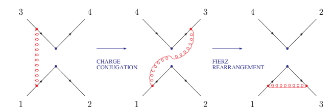
Figure 1: An example of Fierz and charge conjugation rearrangements for Feynman graphs of four-fermion operators.

We have computed the amputated Green’s functions of the four-fermion operators at one loop in two different ways. In the first one we use the Fierz and charge conjugation rearrangements to connect the proper vertices of the four-fermion operators to the bilinear ones. In the second, the calculation has been performed computing the four-quark diagrams directly without any rearrangement of quark legs. To carry out the analytic calculations we have used a set of routines written in the symbolic manipulation language FORM, which are a generalization to the overlap case of the ones used in Refs. [35]. Many of the features of those calculations are also present here. We have numerically integrated the analytic FORM outputs for some values of the $\rho$ parameter and we have successfully checked the results obtained with the first method. This also turns out to be a non-trivial check of the numerical integrations relevant in the Neuberger regularization. The full expressions for the one-loop amputated Green’s functions that we have obtained in a generic covariant gauge are reported in Appendix D, and they can be used to impose any set of renormalization conditions.

Once the results have been rotated in the basis (4), the RI renormalization conditions are imposed by taking the trace the amputated Green’s functions in the Landau gauge [18]

$$\mbox{Tr}\;\mbox{I}\!\!\mbox{P}^{\pm}_{i}\widehat{\Lambda}_{k}^{\pm}=\delta_{ik}\qquad(i,k=1,\cdots,5)\;,$$ (49)

where the projectors $\mbox{I}\!\!\mbox{P}^{\pm}_{i}$ are defined in Appendix C. Using the wave function renormalization $Z^{\mbox{\scriptsize RI}}_{\psi}$ defined in eq. (25) and the definition in (43) we obtain

$$[\widehat{Z}^{\pm}]^{\mbox{\scriptsize RI}}=1-\frac{g_{0}^{2}}{16\pi^{2}}\left[\frac{\widehat{\gamma}^{(0)}}{2}\log(\mu a)^{2}+\widehat{B}^{\pm}+2C_{F}B_{\psi}\right]\;,\\$$

where

$$\widehat{B}^{\pm}=\pmatrix{B^{\pm}_{11}&0&0&0&0\cr 0&B_{22}&\pm B_{23}&0&0\cr 0&\pm B_{32}&B_{33}&0&0\cr 0&0&0&B^{\pm}_{44}&B^{\pm}_{45}\cr 0&0&0&B^{\pm}_{54}&B^{\pm}_{55}\cr}\;,$$ (50)

and the $B^{\pm}_{ij}$ are

$$B^{+}_{11}=\frac{-2(B_{S}-5B_{V})}{3} B^{-}_{11}=\frac{4(B_{S}+B_{V})}{3}$$ (51)

$$B_{22}=-\frac{B_{S}}{3}+3B_{V} B_{23}=-2(B_{S}-B_{V})$$

$$B_{32}=0 B_{33}=\frac{8B_{S}}{3}$$

$$B^{+}_{44}=\frac{23B_{S}+9B_{T}}{12} B^{-}_{44}=\frac{41B_{S}-9B_{T}}{12}$$

$$B^{+}_{45}=\frac{-B_{S}+B_{T}}{12} B^{-}_{45}=\frac{5(B_{S}-B_{T})}{12}$$

$$B^{+}_{54}=\frac{5(B_{S}-B_{T})}{4} B^{-}_{54}=\frac{-B_{S}+B_{T}}{4}$$

$$B^{+}_{55}=\frac{-9B_{S}+41B_{T}}{12} B^{-}_{55}=\frac{9B_{S}+23B_{T}}{12}\;,$$

where the $B_{\Gamma}$’s are reported in Table 1. The relations above are valid in the Landau gauge for any action which preserves chiral symmetry, where $B_{A}=B_{V}$ and $B_{P}=B_{S}$.

The Wilson coefficients and the four-fermion operators of the weak effective Hamiltonian are often defined in one of the $\overline{\mbox{MS}}$ schemes. Unfortunately the definition of the $\overline{\mbox{MS}}$ scheme for the four-fermion operators is not unique even if we consider the Naive Dimensional Regularization only. This is a source of confusion in the literature, where quite often one encounters comparisons of matrix elements that have been computed in different schemes. Incidentally, we note that the $\overline{\mbox{MS}}$-NDR scheme used in the lattice calculation of Ref. [8] differs from the one used in  [37], which moreover is not the one adopted in [38]. In some cases, differences between various schemes may be numerically large. On the other hand the matrix elements of the four-fermion operators in a given scheme are useful only if they are matched with the Wilson coefficients computed in the same scheme. From the perturbative computation of the Wilson coefficients in a given scheme $\chi$, it is straightforward to extract the evolution operator $[\widehat{w}^{\pm}(\mu)]^{\chi}$ at the NLO. Then the corresponding renormalization constants are given by

$$[\widehat{Z}^{\pm}(\mu a)]^{\chi}=[\widehat{w}^{\pm}(\mu)]^{\chi}[\widehat{Z}^{\pm}(a)]^{\mbox{\scriptsize RGI}}=[\widehat{w}^{\pm}(\mu)]^{\chi}[\widehat{w}^{\pm\;\mbox{\scriptsize RI}}(\mu)]^{-1}[\widehat{Z}^{\pm}(\mu a)]^{\mbox{\scriptsize RI}}\;,$$ (52)

where $[\widehat{w}^{\pm}(\mu)]^{\mbox{\scriptsize RI}}$ can be found in [37, 12, 38]. This is equivalent to using only RGI Wilson coefficients and operators as proposed in [12].

5 Conclusions

The matrix elements of dimension-six four-fermion operators without power subtractions are the primary ingredients for studying many interesting phenomenological problems in weak interactions, among which the most important are the predictions of the $K^{0}-\bar{K}^{0}$ and $B^{0}-\bar{B}^{0}$ mixings in the Standard Model and beyond. The renormalization constants of these operators are also relevant for studying the $\Delta I=1/2$ rule and computing the CP-violation parameter $\epsilon^{\prime}/\epsilon$.
In this paper we have studied in detail the mixing of these operators using the overlap lattice regularization proposed by Neuberger and computed their renormalization factors at one loop in perturbation theory. The computations were done in two independent ways: in one case, using Fierz and charge conjugation rearrangements, the four-fermion Green’s functions are given in terms of the one loop results for the bilinear operators; in the other case the Feynman diagrams are computed directly using FORM codes.
We have shown that operators belonging to different chiral representations do not mix among themselves. We have explicitly verified that, as expected, the mixing matrices for the parity-violating and parity-conserving operators are the same. Furthermore, the improvement of the matrix elements is highly simplified by the Ginsparg-Wilson relation and the renormalization constants are the same as the unimproved case. In the Wilson formulation, whether improved or not, the construction of renormalized operators requires subtractions of operators with wrong chirality. These become very severe in the case of power divergences, i.e. $\Delta I=1/2$, $\epsilon^{\prime}/\epsilon$, etc. We believe that the overlap regularization represents a very promising approach for solving these long-standing problems.

Appendix A Feynman Rules

In this appendix we report the Feynman rules used in the computations. Some abbreviations of functions occurring on the lattice are useful:

$$\hat{k}_{\mu} = \frac{2}{a}\sin(\frac{k_{\mu}a}{2})\qquad\hat{k}^{2}=\sum_{0}^{3}\hat{k}_{\mu}^{2}$$

$$\bar{k}_{\mu} = \frac{1}{a}\sin(k_{\mu}a)\qquad\bar{k}^{2}=\sum_{0}^{3}\bar{k}_{\mu}^{2}\;.$$ (53)

The gluonic propagator in a generic covariant gauge is defined as

$$G_{\mu\nu}(k)=\left(\delta_{\mu\nu}+(\alpha-1)\hat{k}_{\mu}\hat{k}_{\nu}/\hat{k}^{2}\right)/\hat{k}^{2}\;,$$ (54)

where $\alpha$ is the gauge parameter.

Let us define some useful matrices in Dirac space:

$$X_{0}(p) = i\gamma_{\mu}\bar{p}_{\mu}-\frac{\rho}{a}+\frac{ar}{2}\hat{p}^{2}$$ (55)

$$X_{1\mu}(p+p^{\prime}) = -ig_{0}\left[\gamma_{\mu}\cos\Big{(}\frac{p_{\mu}+p^{\prime}_{\mu}}{2}a\Big{)}-ir\sin\Big{(}\frac{p_{\mu}+p^{\prime}_{\mu}}{2}a\Big{)}\right]$$

$$X_{2\mu\nu}(p+p^{\prime}) = -a\frac{g_{0}^{2}}{2}\delta_{\mu\nu}\left[r\cos\Big{(}\frac{p_{\mu}+p^{\prime}_{\mu}}{2}a\Big{)}-i\gamma_{\mu}\sin\Big{(}\frac{p_{\mu}+p^{\prime}_{\mu}}{2}a\Big{)}\right]\;.$$

The fermionic propagator of the overlap action is

$$S^{(0)}_{N}(p)=\frac{a}{2\rho}\left[\frac{-i\gamma_{\rho}\bar{p}_{\rho}}{\omega(p)+b(p)}+1\right]=\frac{a}{2\rho}\frac{X_{0}^{\dagger}(p)+\omega(p)}{\omega(p)+b(p)}\;,$$ (56)

with

$$b(p) = \frac{ar}{2}\hat{p}^{2}-\frac{\rho}{a}\;,$$ (57)

$$\omega(p) = \sqrt{\bar{p}^{2}+\left(\frac{ra}{2}\hat{p}^{2}-\frac{\rho}{a}\right)^{2}}\;.$$ (58)

For $0<\rho<2r$ the propagator $S^{(0)}_{N}(p)$ exhibits a massless pole only when $p_{\mu}=0$, and there are no doublers.

The vertices of the overlap Dirac operator are

$$V^{(1)}_{\mu}(p,p^{\prime}) = \frac{\rho}{\omega(p^{\prime})+\omega(p)}\left\{X_{1\mu}\left(p+p^{\prime}\right)-\frac{X_{0}(p^{\prime})}{\omega(p^{\prime})}X_{1\mu}^{\dagger}\left(p+p^{\prime}\right)\frac{X_{0}(p)}{\omega(p)}\right\}$$ (59)

and

$$V^{(2)}_{\mu\nu}(p,p^{\prime}) = \left[\frac{\rho}{\omega(p^{\prime})+\omega(p)}\left\{X_{2\mu\nu}\left(p+p^{\prime}\right)-\frac{X_{0}(p^{\prime})}{\omega(p^{\prime})}X_{2\mu\nu}^{\dagger}\left(p+p^{\prime}\right)\frac{X_{0}(p)}{\omega(p)}\right\}\right.$$

$$+ \frac{\rho}{2\{\omega(p^{\prime})+\omega(p)\}\{\omega(p)+\omega(p+k)\}\{\omega(p+k)+\omega(p^{\prime})\}}$$

$$\times \left\{X_{0}(p^{\prime})X^{\dagger}_{1\mu}\left(p+p^{\prime}+k\right)X_{1\nu}\left(2p+k\right)+X_{1\mu}\left(p+p^{\prime}+k\right)X_{0}^{\dagger}(p+k)X_{1\nu}(2p+k)\right.$$

$$+ X_{1\mu}\left(p+p^{\prime}+k\right)X_{1\nu}^{\dagger}\left(2p+k\right)X_{0}(p)$$

$$- \left.\left.\frac{\omega(p^{\prime})+\omega(p)+\omega(p+k)}{\omega(p^{\prime})\omega(p)\omega(p+k)}X_{0}(p^{\prime})X_{1\mu}^{\dagger}\left(p+p^{\prime}+k\right)X_{0}(p+k)X_{1\nu}^{\dagger}\left(2p+k\right)X_{0}(p)\right\}\right]\;.$$

Appendix B Notations and Fierz Transformations

In this appendix we fix our notations for the color and spin matrices. We also report the formulæ used for Fierz transformations in color and Dirac space.
The Gell-Mann group generators of the $SU(N_{c})$ Lie algebra are denoted by $t^{A},A=1,\dots,N^{2}_{c}-1$. They are Hermitian, traceless $N_{c}\times N_{c}$ matrices and are normalized according to

$$\mbox{Tr}\;(t^{A}t^{B})=\frac{1}{2}\delta^{AB}\;.$$ (61)

They satisfy the commutation relations

$$[t^{A},t^{B}]=if^{ABC}t^{C}\;,\\$$ (62)

where summation over repeated indices is implied. The structure constants $f^{ABC}$ are completely antisymmetric and real. With these conventions the completeness relation for the $t$-generators reads

$$\sum_{A=1}^{N_{c}^{2}-1}(t^{A})_{ab}(t^{A})_{cd}=\frac{1}{2}\left(\delta_{ad}\delta_{bc}-\frac{1}{N_{c}}\delta_{ab}\delta_{cd}\right)\;,$$ (63)

and using the above formulas we get

$$\sum_{A=1}^{N_{c}^{2}-1}(t^{A}t^{A})_{ab} = C_{F}\delta_{ab}\;,$$ (64)

$$\sum_{C,D=1}^{N_{c}^{2}-1}f^{ACD}f^{BCD} = C_{A}\delta^{AB}\;,$$ (65)

with $C_{F}=(N_{c}^{2}-1)/2N_{c}$ and $C_{A}=N_{c}$.

The complete basis of 16 Euclidean Dirac $4\times 4$ matrices is denoted by

$$\Gamma=\{\hbox{1$\!\!$1},\gamma_{\mu},\sigma_{\mu\nu},\gamma_{\mu}\gamma_{5},\gamma_{5}\}\equiv\{S,V,T,A,P\},$$ (66)

where $\gamma_{i}$ are the usual Euclidean Dirac matrices in four dimensions and

$$\sigma_{\mu\nu}=\frac{1}{2}[\gamma_{\mu},\gamma_{\nu}]\;.$$ (67)

The charge conjugation matrix satisfies

$$C\gamma^{T}_{\mu}C^{-1}=-\gamma_{\mu}\;,$$ (68)

and in our basis $C=\gamma_{0}\gamma_{2}$.

Repeated $\Gamma$ matrices imply summation of their Lorenz indices (if any); for example $VV=\sum_{\mu}\gamma_{\mu}\otimes\gamma_{\mu}$, $TT=\sum_{\mu<\nu}\sigma_{\mu\nu}\otimes\sigma_{\mu\nu}$, where the sum is over the 6 independent $\sigma_{\mu\nu}$ matrices only. With these conventions the $\Gamma$ matrices are normalized as

$$SS=1,\ VV=4,\ TT=-6,\ AA=-4,\ PP=1\;,$$ (69)

where summation over Dirac indices is understood.

The Fierz transformation of the Dirac indices of a four-fermion operator is defined as

$${\Gamma}\otimes{\Gamma}\equiv\Gamma_{\alpha\beta}\otimes\Gamma_{\gamma\delta}\rightarrow\left[{\Gamma}\otimes{\Gamma}\right]^{F_{D}}\equiv\Gamma_{\alpha\delta}\otimes\Gamma_{\gamma\beta}\;.$$ (70)

The Euclidean Fierz-transformed Dirac tensor products $\left[{\Gamma}\otimes{\Gamma}\right]^{F_{D}}$ can be re-expressed as a linear combination of the complete set of the original tensor products $\Gamma\otimes\Gamma$ as follows :

$$\left(\begin{array}[]{c}\left[{{S}}\otimes{{S}}\right]^{F_{D}}\\ \left[{{V}}\otimes{{V}}\right]^{F_{D}}\\ \left[{{T}}\otimes{{T}}\right]^{F_{D}}\\ \left[{{A}}\otimes{{A}}\right]^{F_{D}}\\ \left[{{P}}\otimes{{P}}\right]^{F_{D}}\\ \end{array}\right)=-\frac{1}{4}\left(\begin{array}[]{rrrrr}1&1&-1&-1&1\\ 4&-2&0&-2&-4\\ -6&0&-2&0&-6\\ -4&-2&0&-2&4\\ 1&-1&-1&1&1\end{array}\right)\left(\begin{array}[]{c}{S}\otimes{S}\\ {V}\otimes{V}\\ {T}\otimes{T}\\ {A}\otimes{A}\\ {P}\otimes{P}\\ \end{array}\right)\;.$$ (71)

The overall minus sign is due to the anti-commutativity of the Fermi fields.

Appendix C Projectors for Bilinears and Four-Fermion Operators

In this appendix we define the projectors used to impose the RI renormalization conditions for the bilinear and four-fermion operators.

For bilinears the projectors are defined as

$$\mbox{I}\!\!\mbox{P}_{S}=\frac{1}{12}\,I\qquad \qquad\mbox{I}\!\!\mbox{P}_{P}=\frac{1}{12}\,\gamma_{5}$$

$$\mbox{I}\!\!\mbox{P}_{V}=\frac{1}{48}\,\gamma_{\mu}\qquad \qquad\mbox{I}\!\!\mbox{P}_{A}=\frac{1}{48}\,\gamma_{5}\gamma_{\mu}$$

$$\mbox{I}\!\!\mbox{P}_{T}=-\frac{1}{72}\,\sigma_{\mu\nu}\;,$$ (72)

where the identity color matrix is not shown.

If we define

$$\mbox{I}\!\!\mbox{P}_{\Gamma\Gamma}\equiv\Gamma\otimes\Gamma\;,$$ (73)

its trace on a generic four-fermion amputated Green’s function is defined as [18]

$$\mbox{Tr}\;\mbox{I}\!\!\mbox{P}_{\Gamma\Gamma}\Lambda_{\Gamma\Gamma}(p)=\Gamma_{\sigma\rho}\otimes\Gamma_{\sigma^{\prime}\rho^{\prime}}\Lambda_{\Gamma\Gamma}(p)^{RRR^{\prime}R^{\prime}}_{\rho\sigma\rho^{\prime}\sigma^{\prime}},$$ (74)

where the color and spinor indices are explicitly reported and the trace is taken over spin and color. The projectors $\mbox{I}\!\!\mbox{P}^{\pm}_{k}$ for the parity conserving operators $Q^{\pm}_{k}$ are [18]

$$\mbox{I}\!\!\mbox{P}^{\pm}_{1}\equiv+\frac{1}{64N_{c}(N_{c}\pm 1)}(\mbox{I}\!\!\mbox{P}_{VV}+\mbox{I}\!\!\mbox{P}_{AA})$$

$$\mbox{I}\!\!\mbox{P}^{\pm}_{2}\equiv+\frac{1}{64(N_{c}^{2}-1)}(\mbox{I}\!\!\mbox{P}_{VV}-\mbox{I}\!\!\mbox{P}_{AA})\pm\frac{1}{32N_{c}(N_{c}^{2}-1)}(\mbox{I}\!\!\mbox{P}_{SS}-\mbox{I}\!\!\mbox{P}_{PP})$$

$$\mbox{I}\!\!\mbox{P}^{\pm}_{3}\equiv\pm\frac{1}{32N_{c}(N_{c}^{2}-1)}(\mbox{I}\!\!\mbox{P}_{VV}-\mbox{I}\!\!\mbox{P}_{AA})+\frac{1}{16(N_{c}^{2}-1)}(\mbox{I}\!\!\mbox{P}_{SS}-\mbox{I}\!\!\mbox{P}_{PP})$$ (75)

$$\mbox{I}\!\!\mbox{P}^{\pm}_{4}\equiv+\frac{(2N_{c}\pm 1)}{32N_{c}(N_{c}^{2}-1)}(\mbox{I}\!\!\mbox{P}_{SS}+\mbox{I}\!\!\mbox{P}_{PP})\mp\frac{1}{32N_{c}(N_{c}^{2}-1)}\mbox{I}\!\!\mbox{P}_{TT}$$

$$\mbox{I}\!\!\mbox{P}^{\pm}_{5}\equiv\mp\frac{1}{32N_{c}(N_{c}^{2}-1)}(\mbox{I}\!\!\mbox{P}_{SS}+\mbox{I}\!\!\mbox{P}_{PP})+\ \frac{(2N_{c}\mp 1)}{96N_{c}(N_{c}^{2}-1)}\mbox{I}\!\!\mbox{P}_{TT}\;.$$

They are obtained from the tree-level amputated Green’s functions $\Lambda^{\pm(0)}_{k}$ imposing the following orthogonality conditions:

$$\mbox{Tr}\;\mbox{I}\!\!\mbox{P}^{\pm}_{i}\Lambda^{\pm(0)}_{k}=\delta_{ik}\qquad(i,k=1,\dots,5)\;.$$ (76)

The analogous projectors for the parity-violating operators can be found in [18].

Appendix D One-loop results

The one-loop expression for the quark propagator in a generic covariant gauge is

$$S^{-1}=ip\!\!\!/\,\left\{1+\frac{g_{0}^{2}}{16\pi^{2}}C_{F}\Big{[}\alpha L+B_{\psi}+\alpha\,d_{\psi}\Big{]}\right\},$$ (77)

and the amputated Green’s functions of the bilinear operators in a generic covariant gauge are

$$\Lambda_{S} = S\Big{\{}1+\frac{g_{0}^{2}}{16\pi^{2}}C_{F}\Big{[}-(3+\alpha)L+B_{S}-\alpha\,(d_{\psi}-1)\Big{]}\Big{\}}$$

$$\Lambda_{V} = V\Big{\{}1+\frac{g_{0}^{2}}{16\pi^{2}}C_{F}\Big{[}-\alpha\,L+B_{V}-\alpha\,d_{\psi}\Big{]}\Big{\}}-2\frac{g_{0}^{2}}{16\pi^{2}}C_{F}\alpha\frac{p_{\mu}p\!\!\!/}{p^{2}}$$

$$\Lambda_{T} = T\Big{\{}1+\frac{g_{0}^{2}}{16\pi^{2}}C_{F}\Big{[}(1-\alpha)L+B_{T}-\alpha\,(d_{\psi}+1)\Big{]}\Big{\}}\;$$ (78)

$$\Lambda_{A} = A\Big{\{}1+\frac{g_{0}^{2}}{16\pi^{2}}C_{F}\Big{[}-\alpha\,L+B_{A}-\alpha\,d_{\psi}\Big{]}\Big{\}}-2\frac{g_{0}^{2}}{16\pi^{2}}C_{F}\alpha\frac{p_{\mu}p\!\!\!/\gamma_{5}}{p^{2}}$$

$$\Lambda_{P} = P\Big{\{}1+\frac{g_{0}^{2}}{16\pi^{2}}C_{F}\Big{[}-(3+\alpha)L+B_{P}-\alpha\,(d_{\psi}-1)\Big{]}\Big{\}}\;,$$

with $L=\log(pa)^{2}$, and the $B_{\Gamma}$s are reported in Table 1. The terms proportional to the gauge parameter $\alpha$ can be given in simple form as functions of $d_{\psi}=\gamma_{E}-F_{0}-1=-4.792010$ (where $\gamma_{E}$ is the Euler constant and $F_{0}=4.3692252\cdots$). They depend on the gluonic action, and they are independent of the $\rho$ parameter [42], as can be seen using gauge Ward Identities.

The four-fermion operators that we have considered in the “direct” calculation has the form

$$O_{\Gamma_{A}\Gamma_{B}} = \bar{\psi}_{1}\Gamma_{A}\psi_{2}\cdot\bar{\psi}_{3}\Gamma_{B}\psi_{4}$$ (79)

$$O_{\Gamma_{A}^{c}\Gamma_{B}^{c}} = \bar{\psi}_{1}\Gamma_{A}t^{C}\psi_{2}\cdot\bar{\psi}_{3}\Gamma_{B}t^{C}\psi_{4}.$$

The one-loop expressions for the amputated Green’s functions of the parity-conserving operators in a general covariant gauge are

$$\Lambda_{S^{c}S^{c}} = O_{S^{c}S^{c}}+\frac{g_{0}^{2}}{16\pi^{2}}\Bigg{\{}\Big{[}-\frac{1}{2N_{c}}\Big{(}-2(3+\alpha)L+c_{1}-2\alpha(d_{\psi}-1)\Big{)}-N_{c}\Big{(}\alpha L+c_{3}+\alpha\Big{(}d_{\psi}+\frac{1}{2}\Big{)}\Big{)}\Big{]}O_{S^{c}S^{c}}$$

$$+\frac{N_{c}^{2}-1}{N_{c}^{2}}\Big{(}\Big{(}\frac{1}{2}L+c_{2}\Big{)}O_{TT}-\frac{1}{2}\alpha\,\sigma_{\rho\alpha}\otimes\sigma_{\rho\beta}\,\frac{p_{\alpha}p_{\beta}}{p^{2}}\Big{)}$$

$$+\frac{N_{c}^{2}-4}{N_{c}}\Big{(}\Big{(}\frac{1}{2}L+c_{2}\Big{)}O_{T^{c}T^{c}}-\frac{1}{2}\alpha\,\sigma_{\rho\alpha}t^{A}\otimes\sigma_{\rho\beta}t^{A}\,\frac{p_{\alpha}p_{\beta}}{p^{2}}\Big{)}\Bigg{\}}$$

$$\Lambda_{SS} = O_{SS}+\frac{g_{0}^{2}}{16\pi^{2}}\Bigg{\{}\frac{N_{c}^{2}-1}{2N_{c}}\Big{(}-2(3+\alpha)L+c_{1}-2\alpha(d_{\psi}-1)\Big{)}O_{SS}$$

$$+4\Big{(}\Big{(}\frac{1}{2}L+c_{2}\Big{)}O_{T^{c}T^{c}}-\frac{1}{2}\alpha\,\sigma_{\rho\alpha}t^{A}\otimes\sigma_{\rho\beta}t^{A}\,\frac{p_{\alpha}p_{\beta}}{p^{2}}\Big{)}\Bigg{\}}$$

$$\Lambda_{P^{c}P^{c}} = O_{P^{c}P^{c}}+\frac{g_{0}^{2}}{16\pi^{2}}\Bigg{\{}\Big{[}-\frac{1}{2N_{c}}\Big{(}-2(3+\alpha)L+c_{1}-2\alpha(d_{\psi}-1)\Big{)}-N_{c}\Big{(}\alpha L+c_{3}+\alpha\Big{(}d_{\psi}+\frac{1}{2}\Big{)}\Big{)}\Big{]}O_{P^{c}P^{c}}$$

$$+\frac{N_{c}^{2}-1}{N_{c}^{2}}\Big{(}\Big{(}\frac{1}{2}L+c_{2}-\frac{1}{2}\alpha\Big{)}O_{TT}+\frac{1}{2}\alpha\,\sigma_{\rho\alpha}\otimes\sigma_{\rho\beta}\,\frac{p_{\alpha}p_{\beta}}{p^{2}}\Big{)}$$

$$+\frac{N_{c}^{2}-4}{N_{c}}\Big{(}\Big{(}\frac{1}{2}L+c_{2}-\frac{1}{2}\alpha\Big{)}O_{T^{c}T^{c}}+\frac{1}{2}\alpha\,\sigma_{\rho\alpha}t^{A}\otimes\sigma_{\rho\beta}t^{A}\,\frac{p_{\alpha}p_{\beta}}{p^{2}}\Big{)}\Bigg{\}}$$

$$\Lambda_{PP} = O_{PP}+\frac{g_{0}^{2}}{16\pi^{2}}\Bigg{\{}\frac{N_{c}^{2}-1}{2N_{c}}\Big{(}-2(3+\alpha)L+c_{1}-2\alpha(d_{\psi}-1)\Big{)}O_{PP}$$

$$+4\Big{(}\Big{(}\frac{1}{2}L+c_{2}-\frac{1}{2}\alpha\Big{)}O_{T^{c}T^{c}}+\frac{1}{2}\alpha\,\sigma_{\rho\alpha}t^{A}\otimes\sigma_{\rho\beta}t^{A}\,\frac{p_{\alpha}p_{\beta}}{p^{2}}\Big{)}\Bigg{\}}$$

$$\Lambda_{V^{c}V^{c}} = O_{V^{c}V^{c}}+\frac{g_{0}^{2}}{16\pi^{2}}\Bigg{\{}\Big{[}-\frac{1}{2N_{c}}\Big{(}-2\alpha L+c_{4}-2\alpha d_{\psi}\Big{)}-N_{c}\Big{(}\Big{(}\frac{3}{2}+\alpha\Big{)}L+c_{6}+\alpha d_{\psi}\Big{)}\Big{]}O_{V^{c}V^{c}}$$

$$+\Big{(}\frac{2}{N_{c}}+N_{c}\Big{)}\alpha\,\frac{p\!\!\!/t^{A}\otimes p\!\!\!/t^{A}}{p^{2}}$$

$$+\frac{N_{c}^{2}-1}{N_{c}^{2}}\Big{(}\Big{(}\frac{3}{2}L+c_{5}-\alpha\Big{)}O_{AA}+\alpha\,\frac{p\!\!\!/\gamma_{5}\otimes p\!\!\!/\gamma_{5}}{p^{2}}\Big{)}$$

$$+\frac{N_{c}^{2}-4}{N_{c}}\Big{(}\Big{(}\frac{3}{2}L+c_{5}-\alpha\Big{)}O_{A^{c}A^{c}}+\alpha\,\frac{p\!\!\!/\gamma_{5}t^{A}\otimes p\!\!\!/t^{A}\gamma_{5}}{p^{2}}\Big{)}\Bigg{\}}$$

$$\Lambda_{VV} = O_{VV}+\frac{g_{0}^{2}}{16\pi^{2}}\Bigg{\{}\frac{N_{c}^{2}-1}{2N_{c}}\Big{(}\Big{(}-2\alpha L+c_{4}-2\alpha d_{\psi}\Big{)}O_{VV}-4\alpha\,\frac{p\!\!\!/\otimes p\!\!\!/}{p^{2}}\Big{)}$$

$$+4\Big{(}\Big{(}\frac{3}{2}L+c_{5}-\alpha\Big{)}O_{A^{c}A^{c}}+\alpha\,\frac{p\!\!\!/\gamma_{5}t^{A}\otimes p\!\!\!/\gamma_{5}t^{A}}{p^{2}}\Big{)}\Bigg{\}}$$

$$\Lambda_{A^{c}A^{c}} = O_{A^{c}A^{c}}+\frac{g_{0}^{2}}{16\pi^{2}}\Bigg{\{}\Big{[}-\frac{1}{2N_{c}}\Big{(}-2\alpha L+c_{4}-2\alpha d_{\psi}\Big{)}-N_{c}\Big{(}\Big{(}\frac{3}{2}+\alpha\Big{)}L+c_{6}+\alpha d_{\psi}\Big{)}\Big{]}O_{A^{c}A^{c}}$$

$$+\Big{(}\frac{2}{N_{c}}+N_{c}\Big{)}\alpha\,\frac{p\!\!\!/\gamma_{5}t^{A}\otimes p\!\!\!/\gamma_{5}t^{A}}{p^{2}}$$

$$+\frac{N_{c}^{2}-1}{N_{c}^{2}}\Big{(}\Big{(}\frac{3}{2}L+c_{5}-\alpha\Big{)}O_{VV}+\alpha\,\frac{p\!\!\!/\otimes p\!\!\!/}{p^{2}}\Big{)}$$

$$+\frac{N_{c}^{2}-4}{N_{c}}\Big{(}\Big{(}\frac{3}{2}L+c_{5}-\alpha\Big{)}O_{V^{c}V^{c}}+\alpha\,\frac{p\!\!\!/t^{A}\otimes p\!\!\!/t^{A}}{p^{2}}\Big{)}\Bigg{\}}$$

$$\Lambda_{AA} = O_{AA}+\frac{g_{0}^{2}}{16\pi^{2}}\Bigg{\{}\frac{N_{c}^{2}-1}{2N_{c}}\Big{(}\Big{(}-2\alpha L+c_{4}-2\alpha d_{\psi}\Big{)}O_{AA}-4\alpha\,\frac{p\!\!\!/\gamma_{5}\otimes p\!\!\!/\gamma_{5}}{p^{2}}\Big{)}$$

$$+4\Big{(}\Big{(}\frac{3}{2}L+c_{5}-\alpha\Big{)}O_{V^{c}V^{c}}+\alpha\,\frac{p\!\!\!/t^{A}\otimes p\!\!\!/t^{A}}{p^{2}}\Big{)}\Bigg{\}}$$

$$\Lambda_{T^{c}T^{c}} = O_{T^{c}T^{c}}+\frac{g_{0}^{2}}{16\pi^{2}}\Bigg{\{}\Big{[}-\frac{1}{2N_{c}}\Big{(}2(1-\alpha)L+c_{7}-2\alpha(d_{\psi}+1)\Big{)}-N_{c}\Big{(}(2+\alpha)L+c_{9}+\alpha\Big{(}d_{\psi}-\frac{1}{2}\Big{)}\Big{)}\Big{]}O_{T^{c}T^{c}}$$

$$+\frac{N_{c}^{2}-1}{N_{c}^{2}}\Big{(}3L+c_{8}-\frac{3}{2}\alpha\Big{)}(O_{SS}+O_{PP})+\frac{N_{c}^{2}-4}{N_{c}}\Big{(}3L+c_{8}-\frac{3}{2}\alpha\Big{)}(O_{S^{c}S^{c}}+O_{P^{c}P^{c}})\Bigg{\}}$$

$$\Lambda_{TT} = O_{TT}+\frac{g_{0}^{2}}{16\pi^{2}}\Bigg{\{}\frac{N_{c}^{2}-1}{2N_{c}}\Big{(}2(1-\alpha)L+c_{7}-2\alpha(d_{\psi}+1)\Big{)}O_{TT}+4\Big{(}3L+c_{8}-\frac{3}{2}\alpha\Big{)}(O_{S^{c}S^{c}}+O_{P^{c}P^{c}})\;\Bigg{\}}.$$

	$\rho=0.4$	$\rho=1.0$	$\rho=1.7$
$c_{1}$	4.761193	8.939783	12.630887
$c_{2}$	-0.142685	-0.488442	-0.790006
$c_{3}$	-1.524484	-1.539241	-1.575409
$c_{4}$	3.048969	3.078482	3.150818
$c_{5}$	-0.428056	-1.465325	-2.370017
$c_{6}$	-1.952540	-3.004566	-3.945426
$c_{7}$	2.478227	1.124716	-0.009205
$c_{8}$	-0.856112	-2.930650	-4.740034
$c_{9}$	-2.095225	-3.493007	-4.735432

Table 2: Values of the finite constants in Landau gauge.

The $c_{i}$ constants, which take the same values also for the mixings of the parity-violating operators (as we have explicitly verified), are reported in Table 2. They correspond to the values of the finite parts in Landau gauge and, in terms of the finite parts of the bilinears, are:

$$c_{1}=2B_{S} \qquad c_{2}=\frac{B_{T}-B_{S}}{8}\qquad\qquad c_{3}=-\frac{B_{S}+3B_{T}+4B_{V}}{8}$$

$$c_{4}=2B_{V} \qquad c_{5}=\frac{B_{V}-B_{S}}{2}\qquad\qquad c_{6}=-\frac{B_{S}+B_{V}}{2}$$

$$c_{7}=2B_{T} \qquad c_{8}=-\frac{3}{4}(B_{S}-B_{T})\qquad c_{9}=-\frac{1}{4}(3B_{S}+B_{T}).$$ (81)

The coefficients of the logarithms can also be re-expressed in terms of of the anomalous dimensions of the bilinears.

References

• [1] N. Cabibbo, G. Martinelli, R. Petronzio, Nucl. Phys. B244 (1984) 381;
R. C. Brower, M. B. Gavela, R. Gupta, G. Maturana, Phys. Rev. Lett. 53 (1984) 1318;
C. Bernard, Argonne 1984, Proceedings of Gauge Theory on a Lattice, p. 85.
• [2] M. Bochicchio et al., Nucl. Phys. B262 (1985) 331.
• [3] S. Sharpe et al., Nucl. Phys. B286 (1987) 253.
• [4] G. Kilcup, S. Sharpe, R. Gupta, A. Patel, Phys. Rev. Lett. 64 (1990) 25.
• [5] S. R. Sharpe, Nucl. Phys. B (Proc. Suppl.) 53 (1997) 181;
L. Lellouch, hep-ph/9906497.
• [6] C. Bernard et al., Nucl. Phys. B (Proc. Suppl.) 4 (1988) 483.
• [7] E. Franco et al., Nucl. Phys. B317 (1989) 63;
M. B. Gavela et al., Nucl. Phys. B306 (1988) 677.
• [8] S. R. Sharpe, A. Patel, Nucl. Phys. B417 (1994) 307;
T. Bhattacharya, R. Gupta, S. R. Sharpe, Phys. Rev. D55 (1997) 4036.
• [9] M. Crisafulli et al., Phys. Lett. B369 (1996) 325;
L. Conti et al., Phys. Lett. B421 (1998) 273.
• [10] JLQCD Collaboration (S. Aoki et al.), Phys. Rev. D60 (1999) 034511.
• [11] C. R. Allton et al., Phys. Lett. B453 (1999) 30.
• [12] A. Donini, V. Giménez, L. Giusti, G. Martinelli, Phys. Lett. B470 (1999) 233.
• [13] M. Ciuchini et al., JHEP 9810 (1998) 008.
• [14] F. Parodi, P. Roudeau, A. Stocchi, Nuovo Cim. A112 (1999) 833;
F. Caravaglios, F. Parodi, P. Roudeau, A. Stocchi, hep-ph/0002171.
• [15] M. Ciuchini, E. Franco, L. Giusti, V. Lubicz, G. Martinelli, Nucl. Phys. B573 (2000) 201.
• [16] L. Giusti, A. Romanino, A. Strumia, Nucl. Phys. B550 (1999) 3;
R. Barbieri, L. J. Hall, A. Romanino, Nucl. Phys. B551 (1999) 93.
• [17] L. Maiani, G. Martinelli, G. C. Rossi, M. Testa, Nucl. Phys. B289 (1987) 505.
• [18] A. Donini, V. Giménez, G. Martinelli, M. Talevi, A. Vladikas, Eur. Phys. J. C10 (1999) 121.
• [19] P. Hasenfratz, Nucl. Phys. B (Proc. Suppl.) 63A-C (1998) 53.
• [20] P. Hasenfratz, V. Laliena, F. Niedermayer, Phys. Lett. B427 (1998) 125.
• [21] H. Neuberger, Phys. Lett. B417 (1998) 141;
H. Neuberger, Phys. Lett. B427 (1998) 353.
• [22] P. Hasenfratz, Nucl. Phys. B525 (1998) 401.
• [23] M. Lüscher, Phys. Lett. B428 (1998) 342.
• [24] P. H. Ginsparg, K. G. Wilson, Phys. Rev. D25 (1982) 2649.
• [25] T. Chiu, C. Wang, S. V. Zenkin, Phys. Lett. B438 (1998) 321.
• [26] D. Kaplan, Phys. Lett. B288 (1992) 342;
Y. Shamir, Nucl. Phys. B406 (1993) 90;
Y. Shamir, hep-lat/0003024.
• [27] P. Hernández, K. Jansen, M. Lüscher, Nucl. Phys. B552 (1999) 363.
• [28] S. Capitani, M. Göckeler, R. Horsley, P. E. L. Rakow, G. Schierholz,
Phys. Lett. B468 (1999) 150;
S. Capitani, M. Göckeler, R. Horsley, P. E. L. Rakow, G. Schierholz,
Nucl. Phys. B (Proc. Suppl.) 83-84 (2000) 893;
S. Capitani et al., hep-lat/0007004.
• [29] H. Neuberger, Phys. Rev. Lett. 81 (1998) 4060;
R. G. Edwards, U. M. Heller, R. Narayanan, Nucl. Phys. B540 (1999) 457;
A. Bode, U. M. Heller, R. G. Edwards, R. Narayanan, hep-lat/9912043;
P. Hernández, K. Jansen, L. Lellouch, hep-lat/0001008;
R. Narayanan, H. Neuberger, hep-lat/0005004;
S. J. Dong, F. X. Lee, K. F. Liu, J. B. Zhang, hep-lat/0006004;
L. Giusti, C. Hoelbling, C. Rebbi, Nucl. Phys. (Proc. Suppl.) 83-84 (2000) 896 and in preparation.
• [30] M. Beneke, G. Buchalla, I. Dunietz, Phys. Rev. D54 (1996) 4419 and references therein.
• [31] C. Dawson et al., Nucl. Phys. B514 (1998) 313;
M. Testa, JHEP 9804 (1998) 002.
• [32] M. Ciuchini, E. Franco, G. Martinelli, L. Reina, L. Silvestrini, Z. Phys. C68 (1995) 239.
• [33] G. Martinelli, C. Pittori, C.T. Sachrajda, M. Testa, A. Vladikas, Nucl. Phys. B445 (1995) 81.
• [34] C. Alexandrou, E. Follana, H. Panagopoulos, E. Vicari, hep-lat/0002010.
• [35] S. Capitani et al., Nucl. Phys. B570 (2000) 393;
S. Capitani et al., Nucl. Phys. B (Proc. Suppl.) 83 (2000) 232.
• [36] G. Martinelli, Phys. Lett. B141 (1984) 395.
• [37] M. Ciuchini et al., Nucl. Phys. B523 (1998) 501.
• [38] A. J. Buras, M. Misiak, J. Urban, hep-ph/0005183.
• [39] M. Lüscher, S. Sint, R. Sommer, H. Wittig, Nucl. Phys. B491 (1997) 344.
• [40] F. Niedermayer, Nucl. Phys. (Proc.Suppl.) 73 (1999) 105.
• [41] M. Ishibashi, Y. Kikukawa, T. Noguchi, A. Yamada, Nucl. Phys. B576 (2000) 501.
• [42] S. Capitani, hep-lat/0005008.
• [43] V. Gimenez, L. Giusti, F. Rapuano, M. Talevi, Nucl. Phys. B540 (1999) 472.
• [44] A. González-Arroyo, F. J. Yndurain, G. Martinelli, Phys. Lett. B117 (1982) 437; Erratum-ibid. B122 (1983) 486.
• [45] S. Capitani, M. Lüscher, R. Sommer, H. Wittig, Nucl. Phys. B544 (1999) 669.
• [46] D. Becirevic at al., hep-lat/0005013.