BUTP/2000-16

Fixed Point Gauge Actions with Fat Links:
Scaling and Glueballs

Ferenc Niedermayer, Philipp Rüfenacht and Urs Wenger

Institute for Theoretical Physics

University of Bern

Sidlerstrasse 5, CH-3012 Bern, Switzerland

Abstract

A new parametrization is introduced for the fixed point (FP) action in SU(3) gauge theory using fat links. We investigate its scaling properties by means of the static quark-antiquark potential and the dimensionless quantities $r_{0}T_{c}$, $T_{c}/\sqrt{\sigma}$ and $r_{0}\sqrt{\sigma}$, where $T_{c}$ is the critical temperature of the deconfining phase transition, $r_{0}$ is the hadronic scale and $\sigma$ is the effective string tension. These quantities scale even on lattices as coarse as $a\approx 0.3$ fm. We also measure the glueball spectrum and obtain $m_{0^{++}}=1627(83)$ MeV and $m_{2^{++}}=2354(95)$ MeV for the masses of the scalar and tensor glueballs, respectively.

1 Introduction

One way to study quantum field theories beyond perturbation theory is to discretize the Euclidean space-time, using the lattice spacing $a$ as an ultraviolet regulator [1]. Accordingly, the continuum action is replaced by some discretized lattice action. The basic assumption of universality means that the physical predictions – obtained in the continuum limit $a\to 0$ – do not depend on the infinite variety of discretizing the action. At any finite lattice spacing, however, the discretization introduces lattice artifacts. On dimensional grounds one expects that in purely bosonic theories these discretization errors go away as ${\cal O}(a^{2})$, while in theories with fermions as ${\cal O}(a)$.

Sometimes it is stated that the lattice artifacts in pure Yang-Mills theories can be beaten simply by brute force – using the standard Wilson gauge action and a sufficiently small lattice spacing, i.e. by large computer power and memory. This is only partially true – for example when one calculates the pressure of a hot gluon plasma the computer cost grows like $1/a^{10}$ therefore the size of lattice artifacts becomes crucial.

Naturally, one can use the freedom in discretizing the action to minimize the artifacts. It has been shown by Symanzik [2, 3] that the leading lattice artifacts can be cancelled in all orders of perturbation theory by tuning the coefficients of a few dimension $d+2$ operators in bosonic theories (or dimension $d+1$ operators for fermions). This improvement program can be extended to the non-perturbative regime [4, 5].

A different approach, based on renormalization group (RG) ideas [6], has been suggested in ref. [7]. By solving the fixed point (FP) equations for asymptotically free theories one obtains a classically perfect action – i.e. which has no lattice artifacts on the solutions of the lattice equations of motion. (One can say that the FP action is an on-shell tree-level Symanzik improved action to all orders in $a$.) Although it is not quantum perfect, one expects the FP action to perform better in Monte Carlo simulations. This is indeed true in all cases investigated.

The FP approach has been successfully applied to the two-dimensional non-linear $\sigma$-model [7, 8] and the two-dimensional CP³-model [9]. For SU(3) gauge theory the classically perfect FP action has been constructed and tested in [10, 11, 12, 13] and the ansatz has been extended to include FP actions for fermions as well [14, 15, 16]. In the case of SU(2) gauge theory the FP action has been constructed in [17, 18, 19] and its classical properties have been tested on classical instanton solutions, both in SU(2) and SU(3) [20].

The FP action is not unique – it depends on the RG transformation chosen, and it is crucial to optimize the RG transformation to obtain an interaction range of the action as small as possible. The value of the FP action on a given field configuration can be calculated precisely by a classical saddle point equation. However, this step is too slow to embed into a Monte Carlo calculation and one has to invent a sufficiently fast but at the same time accurate enough method to calculate the FP action.

In earlier works on SU(3) gauge theory the parametrization of the FP action used Wilson loops and their powers. We investigate here a new, richer and more flexible parametrization using plaquettes of the original and of smeared (“fat”) links. This describes the FP action more accurately than the loop ansatz. For the RG transformation we choose the one investigated in ref. [13] since the blocking kernel used there (and the resulting FP action) has better properties than the “standard” Swendsen blocking which uses long staples. Here we approximate the same FP action with the new parametrization. We also improve the method of fixing the parameters: besides the known action values (for a given set of configurations) we also fit the known derivatives $\delta{\cal A}^{\text{FP}}(V)/\delta V_{\mu}(n)$, i.e. we have a much larger set of constraints than previously.

Although being much faster than the loop parametrization of comparable richness, this parametrization has a significant overhead compared to the Wilson action. Therefore it is not clear whether it is not better to use in pure gauge theory a faster but less accurate parametrization of the FP action. However, in QCD the cost associated with fermionic degrees of freedom dominates and one can afford a relatively expensive gauge action. In addition, with fermions it is much harder to decrease the lattice spacing, hence it could pay off to have a better gauge action as well. (Of course, because of the ${\cal O}(a)$ artifacts, it is even more important to improve the fermionic part.)

The paper is organized as follows. In section 2 we present the construction and parametrization of the FP action. Section 3 deals with the measurement of the critical couplings $\beta_{c}$ of the deconfining phase transition corresponding to temporal extensions $N_{\tau}=2$, $3$ and $4$, at various spatial volumes. In section 4 we measure the static $q\bar{q}$ potential by using a correlation matrix between different (spatially) smeared gauge strings. In section 5 the scaling properties of the dimensionless quantities $r_{0}T_{c}$, $T_{c}/\sqrt{\sigma}$ and $r_{0}\sqrt{\sigma}$ are presented. In section 6 the low lying glueball spectrum is measured in all symmetry channels. For the Wilson action the lowest lying $0^{++}$ state shows particularly large cut-off effects hence this quantity provides a non-trivial scaling test. Some technical details are collected in appendices A–D.

2 A new parametrization of the FP action for SU(3) lattice gauge theory

2.1 Introduction

In this section we present a new ansatz for the parametrization which is very general and flexible, and which allows to parametrize the FP action using more and more couplings without any further complications. The approach we use is building plaquettes from the original gauge links as well as from smeared (“fat”) links. In this manner we are able to reproduce the classical properties of the FP action better than with the loop parametrization.

The new ansatz is motivated by the success of using fat links in simulations with fermionic Dirac operators [21, 22, 23, 24, 25, 26]. Fat links are gauge links which are locally smeared over the lattice. In this way the unphysical short-range fluctuations inherent in the gauge field configurations are averaged out and lattice artifacts are reduced dramatically.

As mentioned above, earlier parametrizations of FP actions were based on powers of the traces of loop products along generic closed paths. Restricting the set of paths to loops up to length 8 which are fitting in a $2^{4}$ hypercube, one is still left with 28 topologically different loops [11], some of them having a multiplicity as large as 384. In earlier production runs only loops up to length 6 (and their powers) have been used because including length 8 loops increases the computational cost by a factor of $\sim 220$ [19]. Note that in the loop parametrization one needs length 8 loops to describe well small instanton solutions [19, 20].

The new parametrization presented here provides a way around these problems, although the computational overhead is still considerable. We have calculated the expense of the parametrized FP action and compared it to the expense of an optimized Wilson gauge code. The computational overhead amounts to a factor of $\sim 60$ per link update and comes mainly from recalculating the staples in the smeared links affected by the modified link.

2.2 The FP action

We consider SU($N$) pure gauge theory in four dimensional Euclidean space-time on a periodic lattice. The partition function is defined through

$$Z(\beta)=\int dUe^{-\beta{\cal A}(U)},$$ (1)

where $dU$ is the invariant group measure and $\beta{\cal A}(U)$ is some lattice regularization of the continuum action. We can perform a real space RG transformation,

$$e^{-\beta^{\prime}{\cal A}^{\prime}(V)}=\int dU\exp\left\{-\beta({\cal A}(U)+T(U,V))\right\},$$ (2)

where $V$ is the blocked link variable and $T(U,V)$ is the blocking kernel defining the transformation,

$$T(U,V)=-\frac{\kappa}{N}\sum_{n_{B},\mu}\left(\text{Re}\text{Tr}(V_{\mu}(n_{B})Q^{\dagger}_{\mu}(n_{B}))-{\cal N}_{\mu}^{\beta}\right).$$ (3)

Here, $Q_{\mu}(n_{B})$ is a $N\times N$ matrix representing some mean of products of link variables $U_{\mu}(n)$ connecting the sites $2n_{B}$ and $2(n_{B}+\hat{\mu})$ on the fine lattice and ${\cal N}_{\mu}^{\beta}$ is a normalization constant ensuring the invariance of the partition function. By optimizing the parameter $\kappa$, it is possible to obtain an action on the coarse lattice which has a short interaction range. A simple choice for $Q_{\mu}$ is the Swendsen blocking, which contains averaging over the 6 (long) staples along the direction $\mu$. In ref. [13] the averaging was improved by including more paths in $Q_{\mu}$. The main idea of this block transformation is that, instead of using just simple staples, one additionally builds “diagonal staples” along the planar and spatial diagonal directions orthogonal to the link direction. In this way one achieves that each link on the fine lattice contributes to the averaging function and the block transformation represents a better averaging. In this paper we employ the RG transformation of ref. [13], using, however, a completely new parametrization.

On the critical surface at $\beta\rightarrow\infty$, equation (2) reduces to a saddle point problem representing an implicit equation for the FP action ${\cal A}^{\text{FP}}$,

$${\cal A}^{\text{FP}}(V)=\min_{\{U\}}\left\{{\cal A}^{\text{FP}}(U)+T(U,V)\right\}.$$ (4)

The FP equation (4) can be studied analytically up to quadratic order in the vector potentials [13]. However, for solving the FP equation on coarse configurations with large fluctuations one has to resort to numerical methods, and a sufficiently rich parametrization for the description of the solution is required.

2.3 The parametrization

In order to build a plaquette in the $\mu\nu$-plane from smeared links we introduce asymmetrically smeared links $W_{\mu}^{(\nu)}$, where $\mu$ denotes the direction of the link and $\nu$ specifies the plaquette-plane to which they are contributing. This asymmetric smearing suppresses staples which lie in the $\mu\nu$-plane relative to those in the orthogonal planes $\mu\lambda$, $\lambda\neq\nu$. Obviously, these two types of staples play a different role, and we know from the quadratic approximation and the numerical evaluation of the FP action that the interaction is concentrated strongly on the hypercube [13]. Additional details on the smearing and the parametrization are given in appendix A.1.

From the asymmetrically smeared links we construct a “smeared plaquette variable”

$$w_{\mu\nu}=\text{Re\,Tr}\left(1-W_{\mu\nu}^{\text{pl}}\right),$$ (5)

together with the ordinary Wilson plaquette variable

$$u_{\mu\nu}=\text{Re\,Tr}\left(1-U_{\mu\nu}^{\text{pl}}\right),$$ (6)

where

$$W_{\mu\nu}^{\text{pl}}(n) =W_{\mu}^{(\nu)}(n)W_{\nu}^{(\mu)}(n+\hat{\mu})W_{\mu}^{(\nu)\dagger}(n+\hat{\nu})W_{\nu}^{(\mu)\dagger}(n),$$ (7)

and

$$U_{\mu\nu}^{\text{pl}}(n) =U_{\mu}(n)U_{\nu}(n+\hat{\mu})U_{\mu}^{\dagger}(n+\hat{\nu})U_{\nu}^{\dagger}(n).$$ (8)

Finally, the parametrized action has the form

$${\cal A}[U]=\frac{1}{N}\sum_{\mu<\nu}f(u_{\mu\nu},w_{\mu\nu})\,,$$ (9)

where we choose a polynomial in both plaquette variables,

$$f(u,w) = \sum_{kl}p_{kl}u^{k}w^{l}$$ (10)

$$= p_{10}u+p_{01}w+p_{20}u^{2}+p_{11}uw+p_{02}w^{2}+\ldots\,.$$

The coefficients $p_{kl}$, together with the parameters appearing in the smearing (cf. appendix A.1) should be chosen such that the resulting approximation to ${\cal A}^{\text{FP}}$ is sufficiently accurate. Note that the ansatz involves two types of parameters: the coefficients in the asymmetric smearing enter non-linearly into the action while the coefficients $p_{kl}$ enter linearly.

For simulations with the FP action in physically interesting regions it is important to have a parametrization which is valid for gauge fields on coarse lattices, i.e. on typical rough configurations. We turn to this problem in the next section.

2.4 The FP action on rough configurations

The parametrization of the FP action on strongly fluctuating fields is a difficult and delicate problem. In this section we describe briefly the procedure of obtaining a parametrization which uses only a compact set of parameters, but which describes the FP action still sufficiently well for the use in actual simulations. We also provide some details about the fitting procedure employed.

In eq. (4) the minimizing field $U=\overline{U}(V)$ on the fine lattice is much smoother than the original field $V$ on the coarse lattice – its action density is $30-40$ times smaller. This allows an iterative solution of eq. (4) as follows. First one chooses a set of configurations $V$ with sufficiently small fluctuations such that for the corresponding fine field $\overline{U}(V)$ one can use on the rhs. an appropriate starting action (the Wilson action, or better the action ${\cal A}_{0}$, eqs. (A.15) and (A.16) which describes well the FP action in the quadratic approximation). The values ${\cal A}^{\text{FP}}(V)$ obtained this way have to be approximated sufficiently accurately by choosing the free parameters in the given ansatz. Once this is done, one considers a new, rougher set of configurations $V$ for which the fields $\overline{U}(V)$ have fluctuations within the validity range of the previous parametrization and repeats the procedure described. After 3 such steps one reaches fluctuations typical for a lattice spacing $a\approx 0.2-0.3\text{ fm}$.

In previous works only the action values ${\cal A}^{\text{FP}}(V)$ have been fitted in order to optimize the parameters. Here we extend the set of requirements by including into the $\chi^{2}$-function to be minimized the derivatives of the FP action with respect to the gauge links in a given colour direction $a=1,\ldots,N^{2}-1$,

$$\frac{\delta{\cal A}^{\text{FP}}(V)}{\delta V_{\mu}^{a}(n)}\,.$$ (11)

Note that these derivatives are easily calculated from the minimizing configuration since they are given simply by $\delta T(U,V)/\delta V_{\mu}^{a}(n)$ at $U=\overline{U}(V)$. In this way one has $4(N^{2}-1)V$ local conditions for each configuration $V$ instead of a single global condition, the total value ${\cal A}^{\text{FP}}(V)$. (In addition, a good description of local changes is perhaps more relevant in a Monte Carlo simulation with local updates.) An important test for the flexibility of the parametrization is whether both the requirements for fitting the derivatives and the action values can be met at the same time. This is indeed the case.

For addressing questions concerning topology it is crucial that the parametrization describes accurately enough the exactly scale-invariant (lattice) instanton solutions [17, 18, 19, 20]. For this purpose we generate sets of SU(2) single instanton configurations embedded in SU(3) on a $12^{4}$ lattice with instanton radius $\rho/a$ ranging from 3.0 down to 1.1. We then block the configurations down to a $6^{4}$ lattice (using the blocking which defines the RG transformation). As can be seen from figure 1, these are solutions of the FP equations of motion for radii $\rho/a\gtrsim 0.9$. Note that for $\rho/a\lesssim 0.9$ the quantity $T(U,V)$ becomes non-zero, indicating that instantons of that size “fall through the lattice”, i.e. they are no longer solutions. The deviation from scaling at larger radii seen in figure 1 is due to the discontinuity at the boundary of the periodic lattice and is under control.

Figure 1: Action values for SU(2) single instanton solutions $V$ on a $6^{4}$ lattice in units of the continuum instanton action $A_{\text{inst}}$ as a function of the instanton radius $\rho/a$. Note, that $A^{\text{FP}}(V)=A^{\text{FP}}(U)+T(U,V)$, where $U$ is the minimized configuration on the fine lattice.

In the final step, we first fit the derivatives on $\sim 50$ thermal configurations corresponding roughly to a Wilson critical coupling at $N_{\tau}\approx 2$, $\beta_{c}^{W}\approx 5.1$. In the following the non-linear parameters (defining the asymmetric smearing) are kept fixed, while we include in addition the action values and the derivatives of $\sim 75$ thermal configurations at $\beta^{\text{FP}}=$ 2.8, 4.0, 7.0 and the action values of the instanton configurations. The corresponding $\chi^{2}$ is then minimized only in the linear parameters $p_{kl}$.

To assure stability of the fit we check that the $\chi^{2}$ is stable on independent configurations which are not included in the fit. Using high order polynomials of the plaquette variables $u$ and $w$ there is a danger of generating fake valleys in the $uw$-plane (for $u$, $w$ values which are not probed by the typical configurations and hence not restricted in $\chi^{2}$). The presence of such regions is dangerous since it can force the system to an atypical – e.g. antiferromagnetic – configuration. We find that this can be circumvented by choosing an appropriate set of parameters. (Note that, as usually when parametrizing the FP action, there are flat directions in the parameter space along which the value of $\chi^{2}$ changes only slightly, i.e. there is a large freedom in choosing the actual parameters.)

The smallest acceptable set of parameters consists of four non-linear parameters describing the asymmetrically smeared links $W_{\mu}^{(\nu)}$ and fourteen linear parameters $p_{kl}$ with $0<k+l\leq 4$. The values of these parameters are given in appendix A.4 and fulfill the correct normalization. They form the final approximation of the FP action.

Compared to the loop parametrization of ref. [13] the present parametrization gives a deviation from the true FP action values smaller by a factor of 2 for configurations which are typical for the range of lattice spacing $0.03\text{ fm}\lesssim a\lesssim 0.2\text{ fm}$. It also describes scale invariant lattice instantons for $\rho/a\approx 1.1$ to a precision better than 2%. Note that this parametrization is not intended to be used on extremely smooth configurations. In order to be able to describe the typical (large) fluctuations by a relatively simple ansatz we did not implement the ${\cal O}(a^{2})$ Symanzik conditions (cf. appendix A.2) in the last step. In the intermediate steps (i.e. for smaller fluctuations), however, our parametrization (containing non-constant smearing coefficients $\eta(x)$, $c_{i}(x)$) is optimized under the constraint to satisfy the ${\cal O}(a^{2})$ Symanzik conditions as well.

In our Monte Carlo simulations we use only the final parametrization with constant $\eta$ and $c_{i}$. The parameters of the intermediate approximations to the FP action are not given here.

To investigate the lattice artifacts with our parametrization, we perform a number of scaling tests, which are described in the subsequent sections.

3 The critical temperature of the deconfining phase transition

3.1 Details of the simulation

Using the parametrized FP action we perform a large number of simulations on lattices with temporal extension $N_{\tau}=2$, $3$ and 4 at three to six different $\beta$-values near the estimated critical $\beta_{c}$. Various spatial extensions $N_{\sigma}/N_{\tau}=2.5\ldots 5$ are explored with the intention of examining the finite size scaling of the critical couplings. Configurations are generated by alternating Metropolis and overrelaxation updates.

In the equilibrated system we measure the Polyakov loops averaged over the whole lattice,

$$L\equiv\frac{1}{N_{\sigma}^{3}}\sum_{\vec{x}}\text{Tr}\prod_{t=0}^{N_{\tau}-1}U_{4}(\vec{x},t),$$ (12)

as well as the action value of the configuration after each sweep. Both values are stored for later use in a spectral density reweighting procedure.

The details of the simulation and the run parameters are collected in tables C.1, C.2 and C.3, where we list the lattice size together with the $\beta$-values and the number of sweeps. However, near a phase transition the number of sweeps is an inadequate measure of the collected statistics, because the resulting error is strongly influenced by the persistence time and the critical slowing down. The persistence time of one phase is defined as the number of sweeps divided by the observed number of flip-flops between the two phases [27]. This quantity makes sense only for $\beta$-values near the critical coupling $\beta_{c}$ and has to be taken with care: for the small volumes which we explore, the fluctuations within one phase can be as large as the separation between the two phases, and the transition time from one state to the other is sometimes as large as the persistence time itself. The estimated persistence time $\tau_{p}$ and the integrated autocorrelation time $\tau_{\text{int}}$ of the Polyakov loop operator are listed in the last two columns in tables C.1, C.2 and C.3.

3.2 Details of the analysis

For the determination of the critical couplings in the thermodynamic limit we resort to a two step procedure. First we determine the susceptibility of the Polyakov loops,

$$\chi_{L}\equiv V_{\sigma}\left(\langle|L|^{2}\rangle-\langle|L|\rangle^{2}\right),\quad V_{\sigma}=N_{\sigma}^{3},$$ (13)

as a function of $\beta$ for a given lattice size and locate the position of its maximum. In the thermodynamic limit the susceptibility develops a delta function singularity at a first order phase transition. On a finite lattice the singularity is rounded off and the quantity reaches a peak value $\chi_{L}^{\text{peak}}$ at some $\beta_{c}(V_{\sigma})$.

The critical coupling, i.e. the location of the susceptibility peak, is determined by using the spectral density reweighting method, which enables the calculation of observables away from the values of $\beta$ at which the actual simulations are performed. This method has been first proposed in [28, 29] and has been developed further by Ferrenberg and Swendsen [30, 31].

In a second step we extrapolate the critical couplings for each value of $N_{\tau}$ to infinite spatial volume using the finite size scaling law for a first order phase transition,

$$\beta_{c}(N_{\tau},N_{\sigma})=\beta_{c}(N_{\tau},\infty)-h\left(\frac{N_{\tau}}{N_{\sigma}}\right)^{3},$$ (14)

where $h\approx 0.1$ is considered to be a universal quantity independent of $N_{\tau}$ [32]. In figure 2 we show the susceptibility $\chi_{L}$ as a function of $\beta$. The solid lines are the interpolations obtained by the reweighting method and the dashed lines represent the bootstrap error band estimations. For the interpolations at a given lattice size we use the data at all beta values listed in tables C.1–C.3, although the runs at $\beta$-values far away from the critical coupling do not influence the final result.

In table 1 we display the values of $\beta_{c}(V_{\sigma})$ together with their extrapolations to $V_{\sigma}\to\infty$ according to formula (14).

Figure 2: The Polyakov loop susceptibility on lattices of size $4\times 12^{3}$, $3\times 12^{3}$, $3\times 10^{3}$ and $2\times 10^{3}$. The solid curves are the interpolations using the spectral density reweighting, the dashed lines show the bootstrap error bands.

$N_{\sigma}$	$\beta_{c}(N_{\tau}=2)$	$\beta_{c}(N_{\tau}=3)$	$\beta_{c}(N_{\tau}=4)$
6	2.3552(24)
8	2.3585(12)	2.6826(23)
10	2.3593(7)	2.6816(12)	2.9119(31)
12		2.6803(10)	2.9173(20)
14			2.9222(20)
$\infty$	2.3606(13)	2.6796(18)	2.9273(35)
$h$	0.14(9)	-0.05(7)	0.25(9)

Table 1: Results of the critical couplings $\beta_{c}$ from the peak location of the Polyakov loop susceptibility and the corresponding infinite volume limit obtained according to relation (14). The finite size scaling constant $h$ is also given.

4 Scaling of the static quark-antiquark potential

4.1 Introduction

An important part of lattice simulations is the determination of the actual lattice spacing $a$ in order to convert dimensionless quantities measured on the lattice into physical units. From the static $q\bar{q}$ potential one usually determines $a$ in units of the string tension $\sigma$ or in units of the hadronic scale $r_{0}$. Using the string tension to set the scale is plagued by some difficulties. Since the noise/signal ratio increases rapidly with increasing $r$, the part of the potential $V(r)$ from which the linear behaviour $\sigma r$ has to be extracted is measured with larger statistical errors. Further, due to the fact that the excited string has a small energy gap at large $q\bar{q}$ separations, it is difficult to resolve the ground state, and this can lead to a systematic error which increases the obtained value of the string tension.

The use of the quantity $r_{0}$ circumvents these problems. In [33] a hadronic scale $r_{c}$ has been introduced through the force $F(r)$ between static quarks at intermediate distances $0.2\,\text{fm}\lesssim r\lesssim 1.0\,\text{fm}$, where one has best information available from phenomenological potential models [34, 35] and where one gets most reliable results on the lattice. One has

$$r_{c}^{2}V^{\prime}(r_{c})=r_{c}^{2}F(r_{c})=c,$$ (15)

where originally [33] $c=1.65$ has been chosen yielding a value $r_{0}\approx 0.49\,\text{fm}=(395\,\text{MeV})^{-1}$ from the potential models. However, on coarse lattices also this alternative way of setting the scale has its ambiguities as will be discussed in section 5.2.

Referring to precision measurements of the low-energy reference scale in quenched lattice QCD with the Wilson action [36, 37, 38] we collect values for $c$ and $r_{c}$ in table 2. The first line is calculated from data in [36] while the two last lines are taken from [37].

$r_{c}/r_{0}$	c
0.662(1)	0.89
1.00	1.65
1.65(1)	4.00
2.04(2)	6.00

Table 2: Parameter values for the determination of the hadronic scale through eq. (15).

The scaling of our parametrized FP action is examined by measuring the static $q\bar{q}$ potential and comparing the quantity $r_{0}\left(V(r)-V(r_{0})\right)$ versus $r/r_{0}$ at several values of $\beta$.

From the potential one can calculate $r_{0}$ and the effective string tension $\sigma$. Finally one can test the scaling of the dimensionless combinations $r_{0}T_{c}$, $T_{c}/\sqrt{\sigma}$ and $r_{0}\sqrt{\sigma}$. This will be described in the next sections.

The scaling checks will be pushed to the extreme by exploring the behaviour of the FP action on coarse configurations with very large fluctuations corresponding to $a\approx 0.3$ fm. This situation is not relevant for practical applications, and it becomes indeed more and more difficult to measure physical quantities due to the very small correlation length and rapidly vanishing signals. Nevertheless, it is still interesting to investigate this situation in order to estimate the region in which the classical approximation to the renormalization group trajectory is still valid.

For the standard plaquette action the static potential on coarse lattices shows strong violations of rotational symmetry [11, 39, 40] and, before fitting it with a function of $r$, usually an empirical term (the lattice Coulomb potential minus $1/r$) is subtracted with an appropriate coefficient. On the contrary, for the FP action of ref. [13], due to the proper choice of the RG transformation the resulting potential is (practically) rotational invariant. Here we do not aim at testing the rotational invariance of the potential but rather at determining $r_{0}$ and $\sigma$.

4.2 Details of the simulation

We perform simulations with the FP action at six different $\beta$-values, of which three correspond to the critical couplings determined in section 3. Configurations are updated by alternating Metropolis with overrelaxation sweeps. The spatial extent of the lattices is chosen to be at least $\sim 1.5$ fm, based on observations in [36, 37, 41]. Table C.4 contains the values of the couplings, the lattice sizes and the number of measurements.

In order to enhance the overlap with the physical ground state of the potential we exploit smearing techniques. The smoothing of the spatial links has the effect of reducing excited-state contaminations in the correlation functions of the strings in the potential measurements. The operators which we measure in the simulations are constructed using the spatial smearing of [42]. It consists of replacing every spatial link $U_{j}(n)$, $j=$ 1, 2, 3 by itself plus a sum of its neighbouring spatial staples and then projecting back to the nearest element in the SU(3) group:

$${\cal S}_{1}U_{j}(x) \equiv {\cal P}_{\text{SU(3)}}\Big{\{}U_{j}(x)+\lambda_{s}\sum_{k\neq j}(U_{k}(x)U_{j}(x+\hat{k})U_{k}^{\dagger}(x+\hat{j})$$

$$\hskip 56.9055pt+U_{k}^{\dagger}(x-\hat{k})U_{j}(x-\hat{k})U_{k}(x-\hat{k}+\hat{j}))\Big{\}}.$$

Here, ${\cal P}_{\text{SU(3)}}Q$ denotes the unique projection onto the SU(3) group element $W$ which maximizes $\text{Re}\text{Tr}(WQ^{\dagger})$ for an arbitrary $3\times 3$ matrix $Q$. The smeared and SU(3) projected link ${\cal S}_{1}U_{j}(x)$ retains all the symmetry properties of the original link $U_{j}(x)$ under gauge transformations, charge conjugation, reflections and permutations of the coordinate axes. The set of spatially smeared links $\{{\cal S}_{1}U_{j}(x)\}$ forms the spatially smeared gauge field configuration. An operator $\cal O$ which is measured on a $n$-times iteratively smeared gauge field configuration is called an operator on smearing level ${\cal S}_{n}$, or simply ${\cal S}_{n}{\cal O}$. In the simulation of the static $q\bar{q}$ potential we use smearing levels with $n=$ 0, 1, 2, 3, 4. The smearing parameter is chosen to be $\lambda_{s}=0.2$ in all cases.

The correlation matrix of spatially smeared strings is constructed in the following way. At fixed $\tau$ we first form smeared string operators along the three spatial axes, connecting $\vec{x}$ with $\vec{x}+r\hat{i}$,

$${\cal S}_{n}V_{i}(\vec{x},\vec{x}+r\hat{i};\tau)=\\ {\cal S}_{n}U_{i}(\vec{x},\tau){\cal S}_{n}U_{i}(\vec{x}+\hat{i},\tau)\ldots{\cal S}_{n}U_{i}(\vec{x}+(r-1)\hat{i},\tau),\quad i=1,2,3,$$ (17)

and unsmeared temporal links at fixed $\vec{x}$, connecting $\tau$ with $\tau+t$,

$$V_{4}(\tau,\tau+t;\vec{x})=U_{4}(\vec{x},\tau)U_{4}(\vec{x},\tau+1)\ldots U_{4}(\vec{x},\tau+(t-1)).$$ (18)

Finally, the correlation matrix is given by

$$C_{lm}(r,t)=\Big{\langle}\sum_{\vec{x},\tau}\sum_{i=1}^{3}\text{Tr}\,{\cal S}_{l}V_{i}(\vec{x},\vec{x}+r\hat{i};\tau)V_{4}(\tau,\tau+t;\vec{x}+r\hat{i})\\ {\cal S}_{m}V_{i}^{\dagger}(\vec{x},\vec{x}+r\hat{i};\tau+t)V_{4}^{\dagger}(\tau,\tau+t;\vec{x})\Big{\rangle}\,,$$ (19)

where $\langle.\rangle$ denotes the Monte Carlo average. In the following the correlation matrices are analyzed as described in section 4.3.

4.3 Details of the analysis and results

In order to extract the physical scale through equation (15) we need an interpolation of the potential and correspondingly the force between the quarks for arbitrary distances $r$. This interpolation of $V(r)$ is achieved by fitting an ansatz of the form

$$V(r)=V_{0}-\frac{\alpha}{r}+\sigma r$$ (20)

to the measured potential values.

We determine the scale in two steps. First we employ the variational techniques described in appendix B using the correlation matrix defined in eq. (19) for a given separation $r$. This method results in a linear combination of string operators ${\cal S}_{n}V$, $n=0,\ldots,4$, which projects sufficiently well onto the ground state of the string, i.e. eliminates the closest excited string states. We then build a $\chi^{2}$ function using the covariance matrix which incorporates correlations between $C_{lm}(t)$ and $C_{l^{\prime}m^{\prime}}(t^{\prime})$. Based on effective masses and on the $\chi^{2}$ values we choose a region $t_{\text{min}}(r)\leq t\leq t_{\text{max}}(r)$. (Too small $t$ values can distort the results due to higher states which are not projected out sufficiently well, while too large $t$ values are useless due to large errors.) In this window we fit the ground state correlator by the exponential form $Z(r)\exp(-tV(r))$, checking the stability under the variation of different parameters of the procedure. The results of these fits are collected in table C.6.

A straightforward strategy is to fit the obtained values of $V(r)$ by the ansatz (20). However, one can decrease the errors on $\alpha$ and $\sigma$ by exploiting the fact that the errors of $V(r)$ at different values of $r$ are correlated. Therefore, in the second step, we use the projectors to the ground state of the string for each $r$, obtained in the first step, and calculate the ground state correlator $\bar{C}(r,t)$ from the correlation matrix $C_{lm}(r,t)$. After this we estimate the covariance matrix $\text{Cov}(r,t;r^{\prime},t^{\prime})$ from the bootstrap samples of $\bar{C}(r,t)$ and use this to build a $\chi^{2}$ function, fitting $\bar{C}(r,t)$ with the expression $Z(r)\exp(-t(V_{0}-\alpha/r+\sigma r))$. We use the fit range $t_{\text{min}}(r)\leq t\leq t_{\text{max}}(r)$ determined in the first step. The fit range in $r$ is determined by examining the $\chi^{2}$ values and the stability of the fitted parameters. The results of these fits are given in table C.5.

Having in hand a global interpolation of the static potential for each $\beta$-value, we are able to determine the hadronic scale $r_{0}$ in units of the lattice spacing through eq. (15). The value of $c$ is chosen appropriate to the coarseness of the lattice and the fit range in $r$.

In addition, we repeat the second step, but restricting this time the values of $r$ to values close to $r_{c}$ to have a local fit to $V(r)$ [33, 38]. This fit is used then again to determine $r_{c}/a$ (and accordingly $r_{0}/a$) from the relation (15).

The final results for $r_{0}/a$ are listed in table 3 where the first error denotes the purely statistical error. The second one represents an estimate of the systematic error and marks the minimal and maximal value of $r_{0}/a$ obtained with different local fit ranges and different reasonably chosen values of $c$. These ambiguities are discussed in detail in section 5.2.

$\beta$	$N_{\tau}$	2cm$r_{0}/a$
3.400		$4.833(39)(\genfrac{}{}{0.0pt}{}{+18}{-22})$
3.150		$3.717(23)(\genfrac{}{}{0.0pt}{}{+16}{-17})$
2.927	4	$2.969(14)(\genfrac{}{}{0.0pt}{}{+5}{-14})$
2.860		$2.740(10)(\genfrac{}{}{0.0pt}{}{+17}{-31})$
2.680	3	$2.237(7)(\genfrac{}{}{0.0pt}{}{+11}{-33})$
2.361	2	$1.500(5)(\genfrac{}{}{0.0pt}{}{+29}{-14})$

Table 3: The hadronic scale $r_{0}/a$ determined from local fits to the potential. The first error denotes the statistical error and the second is the estimate of the systematic error.

In figure 3 we display the potential values. The dashed line is obtained by a simultaneous fit to all the data respecting the previously chosen fit ranges in $r$. The dotted line representing the result of [43] (obtained on anisotropic lattices using an improved action) is hardly distinguishable from our dashed line.

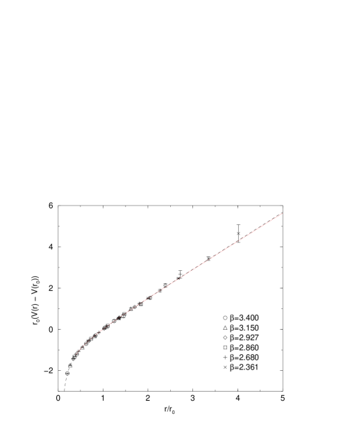
Figure 3: Scaling of the static $q\bar{q}$ potential $V(r)$ expressed in terms of the hadronic scale $r_{0}$. The unphysical constant $r_{0}V(r_{0})$ is subtracted for each lattice spacing such that the curves match at $r/r_{0}=1$. The dashed line is a fit of the form (20) to the data. The dotted line, which practically coincides with our fit, is from [43].

It could be useful to have an empirical interpolating formula connecting the lattice spacing to the bare coupling. (Analogous fits for the Wilson action are given in refs. [37, 38].) The expression

$$\ln(a/r_{0})=-1.1622(24)-1.0848(95)(\beta-3)+0.156(17)(\beta-3)^{2}$$ (21)

describes well the data points in the range $2.361\leq\beta\leq 3.4$. The fit is shown in figure 4.

Figure 4: The measured data points of $\ln(a/r_{0})$ (circles) and their phenomenological description in terms of a polynomial quadratic in $\beta$ (solid line). The plotted points are the values of $r_{0}/a$ from local fits.

5 Scaling of the critical temperature and $r_{0}\sqrt{\sigma}$

To further study the scaling properties of the FP action we examine the dimensionless combinations of physical quantities $T_{c}/\sqrt{\sigma}$, $r_{0}T_{c}$ and $r_{0}\sqrt{\sigma}$.

In this section we present and discuss the results for the FP action and compare them to results obtained for the Wilson action and different improved actions whenever it is possible.

5.1 $T_{c}/\sqrt{\sigma}$

Let us first look at the ratio $T_{c}/\sqrt{\sigma}$, the deconfining temperature in terms of the string tension.

action	$\beta$	$T_{c}/\sqrt{\sigma}$
FP action	2.927	0.624(7)
	2.680	0.622(8)
	2.361	0.628(11)
Wilson [32]	$\infty$	0.630(5)
$1\times 2$ [32]	$\infty$	0.634(8)
DBW2 [44]	$\infty$	0.627(12)
Iwasaki [45]	$\infty$	0.651(12)
Bliss [46]	$\infty$	0.659(8)

Table 4: Results of the deconfining temperature in units of the string tension obtained with the FP action and continuum values for different other actions.

In table 4 we collect all available continuum extrapolations together with the results for the FP action. The data obtained with the Wilson action is taken from [32] where they use the $T_{c}$ values at $N_{\tau}=4$ and 6 from [47] and extrapolate finite volume data for $T_{c}$ at $N_{\tau}=8$ and 12 from [47] to infinite volume. For the value of $\sigma$ they use the string tension parametrization given in [37]. The data for the $1\times 2$ tree level improved action is again taken from [32]. The data denoted by RG improved action is obtained with the Iwasaki action [48] and is taken from [45]. We also include the value by Bliss et al. [46] from a tree level and tadpole improved action. Finally we quote the results from the QCD-TARO collaboration [44] obtained with the DBW2 action. The extrapolations to the continuum stem from [49] where a careful reanalysis has been done.

For extracting the string tension we follow a simple approach. As described above, we perform fits to the on-axis potential values only and therefore we are limited to a small number of different fitting ranges. Nevertheless, the values of $\sigma$ obtained this way and quoted in table C.5 are stable and vary only within their statistical errors over the sets of sensibly considered fit ranges. However, the error on $\sigma$ changes considerably, i.e. up to a factor of 5, depending on whether distance $r=1$ is taken into account or not. Just to play safe we neglect distance $r=1$ in the fits, even if the $\chi^{2}$ would allow it.

The values are displayed in figure 5 together with the data as mentioned above. Our data is compatible within one standard deviation with the continuum extrapolation of the Wilson data and we observe scaling of the FP action within the statistical errors over the whole range of coarse lattices corresponding to values of $N_{\tau}=$ 2, 3 and 4.

Figure 5: $T_{c}/\sqrt{\sigma}$ vs. $1/N_{\tau}^{2}$ for different actions.

5.2 $r_{0}T_{c}$

Unfortunately, precise determinations of $r_{0}/a$ are missing in the literature except for the Wilson action [37, 38] and, in contrast to $T_{c}/\sqrt{\sigma}$, we are not able to compare our data to other actions such as the Iwasaki, DBW2 or the $1\times 2$ tree level improved action. In fact, the determination of $r_{0}/a$ is a delicate issue and systematic effects due to different methods of calculating the force can be sizeable. Due to the fact that extracting the derivative of the potential from a discrete set of points is not unique, the intrinsic systematic uncertainty is not negligible at intermediate and coarse lattice spacings $a\gtrsim 0.15$ fm. For example, in an accurate scale determination of the Wilson gauge action in [37] the authors quote a value of $r_{0}/a=2.990(24)$ at $\beta_{W}=5.7$. This is to be compared with $r_{0}/a=2.922(9)$ of ref. [38] for the same action and $\beta$-value. In view of the claim in [37] to have included all systematic errors and the high relative accuracy ($\sim 0.3\%$) of the data in [38], this systematic difference seems to be a serious discrepancy. Even on finer lattices there are ambiguities: at $\beta_{W}=6.2$ the authors of [38] obtain $r_{0}/a=7.38(3)$, while in [50] a value of $r_{0}/a=7.29(4)$ is quoted.

In that sense our results concerning $r_{0}T_{c}$ have to be taken with appropriate care. In table 5 we collect the data for $r_{0}T_{c}$ from our measurements with the FP action together with the data from measurements with the Wilson action. The critical couplings corresponding to $N_{\tau}=$ 4, 6, 8 and 12 are taken from [32] while the values for $r_{0}/a$ are from the interpolating formula in [38]. The quoted errors are purely statistical. The continuum value is our own extrapolation obtained by performing a fit linear in the leading correction term $1/N_{\tau}^{2}$ and discarding the data point at $N_{\tau}=4$. Finally, the values are plotted in figure 6 for comparison.

$N_{\tau}$	Wilson action	FP action
2		0.750(3)
3		0.746(3)
4	0.719(2)	0.742(4)
6	0.739(3)
8	0.745(3)
12	0.746(4)
$\infty$	0.750(5)

Table 5: Results for the critical temperature in terms of the hadronic scale, $r_{0}T_{c}$, from measurements with the Wilson action and the FP action.

Figure 6: $r_{0}T_{c}$ vs. $1/N_{\tau}^{2}$ for the Wilson and the FP action. The empty circles represent data from measurements with the Wilson action and the filled squares denote the results obtained with the FP action. The solid error bars show the purely statistical error, while the dashed ones indicate the systematic error from the ambiguities in determining the force on coarse lattices.

The Wilson action shows scaling violation for $r_{0}T_{c}$ of about $4\%$ at $N_{\tau}=4$, while at $N_{\tau}=6$ it is already smaller than about $1.5\%$. In that sense this quantity provides a high precision scaling test and thus a very accurate computation of the low-energy reference scale $r_{0}/a$ on the $0.5\%$ level is of crucial importance. The lack of data for different actions is an indication that this is indeed a difficult task. Although the required statistics is in principle accessible to us, we do not have full control over the systematic ambiguities in the calculation of $r_{0}/a$ on the required accuracy level. Nevertheless we observe in principle excellent scaling within $1\%$ or two standard deviations for the FP action even on coarse lattices corresponding to $N_{\tau}=3$ and 2, however, this statement is moderated in view of the large systematic uncertainties.

5.3 $r_{0}\sqrt{\sigma}$

To obtain the dimensionless product $r_{0}\sqrt{\sigma}$ we use the values of $r_{0}/a$ in table 3 obtained from local fits and the values of $\sigma$ as determined in section 5.1, where $\sigma$ is determined from the long range properties of the potential.

In table 6 we collect the resulting values of $r_{0}\sqrt{\sigma}$. We can extrapolate to the continuum by performing a fit linear in $(a/r_{0})^{2}$ and obtain $r_{0}\sqrt{\sigma}=1.193(10)$. For comparison we calculate the data for the Wilson action from the interpolating formula for $r_{0}/a$ in [38] and the string tension parametrization in [37]. The continuum extrapolation for the Wilson data is taken from the analysis of Teper in [49].

Wilson action		FP action
$\beta$	$r_{0}\sqrt{\sigma}$	$\beta$	$r_{0}\sqrt{\sigma}$
5.6925	1.148(12)	2.361	1.194(21)
5.8941	1.170(19)	2.680	1.196(15)
6.0624	1.183(13)	2.860	1.190(23)
6.3380	1.185(11)	2.927	1.191(12)
		3.150	1.185(16)
		3.400	1.198(12)
$\infty$	1.197(11)	$\infty$	1.193(10)

Table 6: $r_{0}\sqrt{\sigma}$ for the Wilson and the FP action.

Figure 7 shows the scaling behaviour of $r_{0}\sqrt{\sigma}$ for the Wilson action (empty circles) and the FP action (filled squares) as a function of $(a/r_{0})^{2}$. The error bars are purely statistical and are dominated by the uncertainty from the string tension. Therefore the systematic ambiguities present in $r_{0}/a$ are not visible within the error bars.

The Wilson action shows a scaling violation of about $4\%$ at $\beta=5.6925$ $(N_{\tau}=4)$, while no scaling violation is seen for the FP action even on lattices as coarse as $\beta=2.361$ $(N_{\tau}=2)$. We would like to emphasize that this is a non-trivial result, since $r_{0}/a$ and $\sqrt{\sigma}a$ are determined independently of each other. However, with the data presently available to us it is difficult to extract the string tension with the accuracy needed to see a striking difference to the Wilson action for $\beta$-values corresponding to $N_{\tau}\geq 4$. This is mainly due to the lack of measurements of the off-diagonal potential values.

Figure 7: Scaling behaviour of $r_{0}\sqrt{\sigma}$ for the Wilson action (empty circles) and the FP action (filled squares).

6 Glueballs

6.1 Introduction

Glueballs are the one-particle states of SU($N$) gauge theory. They are characterized by the quantum numbers $J^{PC}$, denoting the symmetry properties with respect to the O(3) rotations (spin), spatial reflection and charge conjugation. However, the lattice regularization does not preserve the continuous O(3) symmetry, only its discrete cubic subgroup, therefore the eigenstates of the transfer matrix are classified according to irreducible representations of the cubic group. There are five such representations: $A_{1}$, $A_{2}$, $E$, $T_{1}$, $T_{2}$, of dimensions 1, 1, 2, 3, 3, respectively. Their transformation properties can be described by polynomials in $x$, $y$, $z$ as follows: $A_{1}\sim\{1\}$, $A_{2}\sim\{xyz\}$, $E\sim\{x^{2}-z^{2},y^{2}-z^{2}\}$, $T_{1}\sim\{x,y,z\}$ and $T_{2}\sim\{xy,xz,yz\}$, where $x$, $y$, $z$ are components of an O(3) vector. In general, an O(3) representation with spin $J$ splits into several representations of the cubic group. Looking at the corresponding polynomials, it is rather obvious that the splitting starts at $J=2$: $(J=0)\to A_{1}$, $(J=1)\to T_{1}$, $(J=2)\to(E,T_{2})$. The full O(3) rotation symmetry is expected to be restored in the continuum limit. This restoration manifests itself e.g. in the fact that a doublet $E$ and a triplet $T_{2}$ (for a given choice of quantum numbers $PC$) become degenerate to form together the $J=2$ states with 5 possible polarizations.

The main obstacle in the computations of glueball masses on the lattice is the fast decay of the signal in the correlation functions of the gluonic excitations, due to the fact that the glueball masses are relatively large ($m_{G}\gtrsim 1.6$ GeV). For this reason a small lattice spacing $a$ is required to follow the signal long enough. On the other hand, the physical lattice volume should be larger than $L\gtrsim 1.2$ fm to avoid finite size effects. This finally results in a large $L/a$ making it hard to obtain the statistics which is usually required. One possible way around this dilemma is the use of anisotropic lattice actions, which have a finer resolution in time direction, $a_{\tau}\ll a_{\sigma}$, and where one can follow the signal over a larger number of time slices. Although this idea is not new [51], it has been revived only recently by Morningstar and Peardon [52, 53]. Using an anisotropic improved lattice action they investigated the glueball spectrum below 4 GeV in pure SU(3) gauge theory and improved the determinations of the glueball masses considerably compared to previous Wilson action calculations. Recent calculations with the Wilson action comprehend works by the UKQCD collaboration [54] and the GF11 group [55, 56]. It can be said that all three calculations are in reasonable agreement on the masses of the two lowest lying $0^{++}$ and $2^{++}$ glueballs.

Despite this agreement, Wilson action calculations of the $0^{++}$ glueball mass show huge lattice artifacts of around 40 % at $a\approx 0.15$ fm and still 20 % even at $a\approx 0.10$ fm. From this point of view the $0^{++}$ glueball mass is particularly interesting, besides its physical relevance, since it provides an excellent test object on which the scaling behaviour of different actions can be checked and the achieved reduction of discretization errors can be sized. In this sense let us emphasize that our intention here is twofold: firstly, our calculation provides a new and independent determination of glueball masses using FP actions, and secondly, we aim at using the glueball spectrum, in particular the mass of the $0^{++}$ glueball, as another scaling test of the FP action. Although we observe that the FP action scales well in quantities like $r_{0}T_{c}$, $T_{c}/\sqrt{\sigma}$ or $r_{0}\sqrt{\sigma}$, lattice artifacts could be, in principle, quite different for other physical quantities, in particular $r_{0}m_{G}$ or $m_{G}/\sqrt{\sigma}$.

This section is organized as follows. In subsection 6.2 we describe the details of the simulations including the generation of the gauge field configurations and the measurements of the operators. The extraction of masses from the Monte Carlo estimates of glueball correlation functions is described in subsection 6.3. Finally, subsection 6.4 contains the results of our glueball measurements.

6.2 Details of the simulation

We perform simulations at three different lattice spacings in the range $0.1\,\text{fm}\leq a\leq 0.18\,\text{fm}$ and volumes between (1.4 fm)³ and (1.8 fm)³. The simulation parameters for our runs are given in table C.7.

The gauge field configurations are updated by performing compound sweeps consisting of alternating over-relaxation and standard Metropolis sweeps.

First, a rather small preliminary simulation at $\beta=2.86$ is performed. Using the results of some pilot runs, we determine a set of five loop shapes which have large contributions to the $A_{1}^{++}$ channel. Using the labelling of Berg and Billoire [57] these are the length-8 loop shapes 2, 4, 7, 10, 18. They are measured on five smearing levels ${\cal S}_{n}$, $n=2,4,\ldots,10$ with smearing parameter $\lambda_{s}=0.2$ and subsequently projected into the $A_{1}^{++}$ channel.

In the two large simulations at $\beta=3.15$ and 3.40 we measure all 22 Wilson loop shapes up to length eight (see [57]) on the same smearing levels mentioned before and project them into all 20 irreducible glueball channels.

A considerable part of the simulation time is used to measure all the 22 loop shapes. Some of them may turn out to be superfluous in the sense that they give a much worse signal/noise ratio than the others. On the other hand, one is interested in having a set of operators as large as possible to build up the wave function of the lowest glueball state (more precisely, to cancel the unwanted contributions from the neighbouring states in the spectrum). Having measured all these operators will allow us to identify the important loop shapes to be used in future simulations.

The projections of the loop shapes into the irreducible representations of the cubic group are done according to the descriptions in [57, 58]. The correlation matrix elements are then constructed from the projected operators and Monte Carlo estimates are obtained by averaging the measurements in each bin. We measure all possible polarizations in a given channel and add them together in the correlation matrix. This eventually suppresses the statistical noise more than just increasing the statistics since the different polarizations are anti-correlated.

For the extraction of the glueball masses in the $A_{1}^{++}$ representation (which has the same quantum numbers as the vacuum) one has to consider vacuum-subtracted operators. For this purpose we also measure the expectation values of all the operators.

6.3 Details of the analysis

The glueball masses are extracted using the variational techniques described in appendix B. Let us put some remarks which are related to the analysis of the glueball masses in particular.

As we are measuring a large number of operators (up to 145), normally some of them contain large statistical noise. Therefore we only keep a set of well measured operators, on which the whole procedure is numerically stable and well defined.

Another remark concerns the vacuum subtraction necessary in the $A_{1}^{++}$ channel. To obtain vacuum-subtracted operators one usually considers $\phi^{\text{sub}}(\tau)=\phi(\tau)-\langle 0|\phi(\tau)|0\rangle$. However, we follow a different strategy and treat the vacuum on the same footing as the other states in the vacuum channel. As it turns out, the vacuum state can be separated in this procedure with very high accuracy and it is safe to consider only the operator basis orthogonal to the vacuum in the fitting procedure. For this purpose we cut out the vacuum state obtained from solving the generalized eigenvalue equation (B.3), i.e. we only consider the correlation matrix

$$C^{K}_{ij}(t)=(v_{i},C^{M}(t)v_{j}),$$ (22)

with $i,j$ running from $i,j=2,\ldots,K\leq M$ in the further analysis ($i=1$ being the vacuum state). In our experience this strategy yields the most stable subtraction of the vacuum contribution with respect to the statistical fluctuations of the subtracted operators.

In the last step for extracting the glueball masses the large correlation matrix is truncated to a $1\times 1$ or $2\times 2$ matrix, which is subsequently fitted in the fit range $t_{\text{min}}\ldots t_{\text{max}}$ taking both temporal correlations and correlations among the operators into account. The corresponding covariance matrix is calculated from jackknife samples and the error is estimated using a jackknife procedure. The choice of $t_{\text{max}}$ is not crucial and is usually taken according to the relative error of the matrix elements under consideration and the $\chi^{2}$-function. More important is the correct choice of $t_{\text{min}}$. Since excited glueball states are rather heavy we do not expect large contamination of the ground state correlators from excited states even on time slice $t=1$ and therefore $t_{\text{min}}=1$ is usually chosen. In particular this choice is safe if we fix $t_{0}=1$ and $t_{1}=2$ rather than $t_{0}=0$ and $t_{1}=1$ in the variational method, eq. (B.3). Indeed, in the former case the $\chi^{2}$-function remains more stable when we increase $t_{\text{min}}=1$ to $t_{\text{min}}=2$ as a check for the consistency of the resulting masses (as an example take the results in table C.8).

6.4 Results

The results of the fits to the glueball correlators are collected in the appendix in tables C.8 – C.10. We include the results of different fitting ranges in $t$ in the tables in order to give an impression of the stability of the fits. In each channel the result highlighted in boldface is our final choice and represents a most reasonable mass for the given channel. These final mass estimates in units of the lattice spacing are collected in table C.11.

To compare the values it is convenient to use $r_{0}$ to set the scale. In table C.12 we list our estimates of the glueball masses expressed in terms of $r_{0}$, while figure 8 and 9 show our values for the $A_{1}^{++}$ and the $E^{++}$, $T_{2}^{++}$ channels, respectively, together with results from different calculations with the Wilson action (crosses) [49, 54, 56] and the calculations of Morningstar and Peardon [52, 53] and Liu [59] with a tree level/tadpole improved anisotropic action (empty symbols).

Figure 8: Glueball mass estimates for the $A_{1}^{++}$ channel. Results from simulations of the Wilson action (crosses) and a tree level/tadpole improved anisotropic action (empty circles) are shown together with the results obtained with the FP action (filled circles).

To compare our results to the continuum values of the various collaborations we resort to [60] where the above Wilson action results have been expressed in or converted to units of $r_{0}$ using the interpolating formula for the Wilson action [38] and, whenever necessary, the continuum extrapolation has been redone. Our continuum result for the $0^{++}$ glueball mass is an extrapolation to the continuum using a fit function linear in $(a/r_{0})^{2}$. The data in the other channels does not allow to do an extrapolation, thus we simply quote the masses obtained on the finest lattice ($a=0.10$ fm) in brackets. The comparison of our results to the continuum values of the other groups is listed in tables 7 and 8.

Note that one observes restoration of the degeneracy within the statistical errors for the $2^{++}$ state as well as for the $2^{-+}$ state. All our mass estimates agree with the best earlier results within the statistical errors.

Collab.	$r_{0}m_{0^{++}}$	$r_{0}m_{2^{++}}$	year
UKQCD [54]	4.05(16)	5.84(18)	1993
Teper [49]	4.35(11)	6.18(21)	1998
GF11 [56]	4.33(10)	6.04(18)	1999
M&P [53]	4.21(11)(4)	5.85(2)(6)	1999
Liu [59]	4.23(22)	5.85(23)	2000
FP action	4.12(21)	[5.96(24)]	2000

Table 7: Comparison of the two lowest glueball masses in units of $r_{0}$. Our $2^{++}$ value is not extrapolated to the continuum but is the mass obtained at a lattice spacing $a=0.10$ fm.

Collab.	$r_{0}m_{0^{-+}}$	$r_{0}m_{2^{-+}}$	$r_{0}m_{1^{+-}}$	year
Teper [49]	5.94(68)	8.42(78)	7.84(62)	1998
M&P [53]	6.33(7)(6)	7.55(3)(8)	7.18(4)(7)	1999
FP action	[6.74(42)]	[8.00(35)]	[7.93(78)]	2000

Table 8: Comparison of glueball masses in units of $r_{0}$. Values in brackets denote masses obtained at a lattice spacing $a=0.10$ fm and are not extrapolated to the continuum.

Figure 9: Glueball mass estimates for the $2^{++}$ channel. Results from simulations of the Wilson action (crosses) and a tree level/tadpole improved anisotropic action (empty symbols) are shown together with the results obtained with the FP action (filled symbols). Squares and circles denote the $E^{++}$ and $T_{2}^{++}$ mass estimates, respectively.

Finally we convert the scalar and tensor glueball masses into physical units using $r_{0}\approx 0.49\,\text{fm}=(395\text{MeV})^{-1}$. We obtain 1627(83) MeV for the $0^{++}$ and 2354(95) MeV for the $2^{++}$ glueball mass, respectively. Note that the latter value corresponds to the glueball mass measured at a lattice spacing $a=0.10$ fm.

As mentioned in the introduction, it is well known that glueball masses are difficult to measure on the lattice. Indeed, we can barely resolve higher lying glueball states and measuring excited states becomes impossible at the lattice spacings currently available to us. In this sense we can not really take advantage of the parametrized FP action, which is intended to be used on coarse lattices.

One way around this difficulty is the use of anisotropic lattices, where the lattice spacing in temporal direction is much smaller than in spatial direction, $a_{\tau}\ll a_{\sigma}$. The work on the application of the FP approach to anisotropic lattice gauge actions is in progress [61].

7 Summary

In this work we have presented a new parametrization of the FP action of a specific RGT. It uses simple plaquettes built from single gauge links as well as from smeared (“fat”) links. It reproduces the classical properties of the action excellently and respects approximate scale invariance of instanton solutions. Since in addition to the FP action values we parametrize the derivatives with respect to the gauge fields, local changes of the action in a MC simulation are better represented.

The parametrization has been optimized at lattice spacings suitable for performing simulations on coarse lattices up to $a\approx 0.3$ fm.

For subjecting the action to scaling tests we have determined its critical couplings $\beta_{c}$ on lattices with temporal extensions $N_{\tau}=$ 2, 3 and 4. For each $N_{\tau}$ we have performed simulations on several lattices for a finite size scaling study. Furthermore, we have measured the static quark–antiquark potential at various values of the gauge coupling corresponding to $a\approx 0.1-0.3$ fm. From the potential we have extracted the commonly used reference scale $r_{0}$ and the effective string tension $\sigma$ in order to check the scaling behaviour of the parametrized FP action by means of the dimensionless quantities $r_{0}T_{c}$, $T_{c}/\sqrt{\sigma}$ and $r_{0}\sqrt{\sigma}$. In all the quantities we observe excellent scaling within the statistical errors, even on our coarsest lattices.

Additionally, we have measured the glueball spectrum in all symmetry channels. The $A_{1}^{++}$ channel, which shows particularly large lattice artifacts in measurements with the Wilson gauge action, is an excellent candidate for testing the improvements achieved with the parametrized FP action. We observe scaling of the glueball masses and restoration of the rotational symmetry in the $2^{++}$ and $2^{-+}$ channel within the statistical errors. For the glueball masses we obtain 1627(83) MeV for the $0^{++}$ glueball in the continuum and 2354(95) MeV for the $2^{++}$ glueball at a lattice spacing of $a=0.10$ fm.

Acknowledgements We would like to thank Peter Hasenfratz for useful suggestions and discussions.

Appendix A The parametrization

A.1 Details of the parametrization

Let us introduce the notation $S_{\mu}^{(\nu)}(n)$ for the sum of two staples of gauge links in direction $\mu$ in the $\mu\nu$-plane:

$$S_{\mu}^{(\nu)}(n)=U_{\nu}(n)U_{\mu}(n+\hat{\nu})U_{\nu}^{\dagger}(n+\hat{\mu})\\ +U_{\nu}^{\dagger}(n-\hat{\nu})U_{\mu}(n-\hat{\nu})U_{\nu}(n-\hat{\nu}+\hat{\mu})\,.$$ (A.1)

Besides the usual symmetric smearing, we shall also use a non-symmetric smearing. For the symmetric smearing define

$$Q_{\mu}^{\rm s}(n)=\frac{1}{6}\sum_{\lambda\neq\mu}S_{\mu}^{(\lambda)}(n)-U_{\mu}(n)\,$$ (A.2)

and

$$x_{\mu}(n)={\rm Re\,Tr}\left(Q_{\mu}^{\rm s}(n)U_{\mu}^{\dagger}(n)\right).$$ (A.3)

To build a plaquette in the $\mu\nu$-plane from smeared links we introduce asymmetrically smeared links. First define

$$Q_{\mu}^{(\nu)}=\frac{1}{4}\left(\sum_{\lambda\neq\mu,\nu}S_{\mu}^{(\lambda)}+\eta(x_{\mu})S_{\mu}^{(\nu)}\right)-\left(1+\frac{1}{2}\eta(x_{\mu})\right)U_{\mu}\,.$$ (A.4)

Using these matrices we build the asymmetrically smeared links

$$W_{\mu}^{(\nu)}=U_{\mu}+c_{1}(x_{\mu})Q_{\mu}^{(\nu)}+c_{2}(x_{\mu})Q_{\mu}^{(\nu)}U_{\mu}^{\dagger}Q_{\mu}^{(\nu)}+\ldots\,.$$ (A.5)

Here $\eta(x)$, $c_{i}(x)$ are polynomials:

$$\eta(x_{\mu})=\eta^{(0)}+\eta^{(1)}x_{\mu}+\eta^{(2)}x_{\mu}^{2}+\ldots$$ (A.6)

and

$$c_{i}(x_{\mu})=c_{i}^{(0)}+c_{i}^{(1)}x_{\mu}+c_{i}^{(2)}x_{\mu}^{2}+\ldots.$$ (A.7)

A.2 The ${\cal O}(a^{2})$ Symanzik conditions

In this appendix we derive the ${\cal O}(a^{2})$ Symanzik conditions [2, 3, 62, 63, 64, 65] by considering constant non-Abelian gauge potentials. The formulas apply to general SU($N$).

In the continuum we have one scalar, gauge-invariant dimension-4 operator

$$R_{0} =-\frac{1}{2}\sum_{\mu\nu}{\rm Tr}\left({\cal F}_{\mu\nu}^{2}\right),$$ (A.8)

and three dimension-6 operators:

$$R_{1} =\frac{1}{2}\sum_{\mu\nu}\text{Tr}\left(\left(D_{\mu}{\cal F}_{\mu\nu}\right)^{2}\right),$$ (A.9)

$$R_{2} =\frac{1}{2}\sum_{\mu\nu\lambda}\text{Tr}\left(\left(D_{\mu}{\cal F}_{\nu\lambda}\right)^{2}\right),$$ (A.10)

$$R_{3} =\frac{1}{2}\sum_{\mu\nu\lambda}\text{Tr}\left(D_{\mu}{\cal F}_{\mu\lambda}D_{\nu}{\cal F}_{\nu\lambda}\right).$$ (A.11)

According to Symanzik [2, 3] the ${\cal O}(a^{2})$ lattice artifacts of an action are described by an effective continuum action where to the usual continuum action ($\propto R_{0}$) additional terms proportional to $a^{2}R_{1}$, $a^{2}R_{2}$ and $a^{2}R_{3}$ are added with appropriate coefficients. In fact, the equations of motion are $\sum_{\mu}D_{\mu}{\cal F}_{\mu\lambda}=0$ hence the term with $R_{3}$ can be eliminated by a change of variables, hence does not affect the lattice artifacts in on-shell quantities, e.g. masses. (Note that the static $q\bar{q}$ potential is an off-shell quantity, it depends on the choice of the operators. For such quantities one has to improve the operators as well to get rid of artifacts.) The ${\cal O}(a^{2})$ lattice artifacts of on-shell quantities can be eliminated in all orders of perturbation theory by adding to the original lattice action two additional terms which in the naive continuum limit are proportional to $a^{2}R_{1}$ and $a^{2}R_{2}$, with appropriate coefficients. On the tree level the absence of ${\cal O}(a^{2})$ artifacts means that when one expands the lattice action in powers of $a$, for smooth fields the coefficients of $R_{1}$ and $R_{2}$ vanish. The coefficient of $R_{3}$ is not required to vanish (and usually it does not for the FP action).

For the specific lattice gauge action ansatz considered in section 2.3 one obtains

$$\sum_{\mu<\nu}w_{\mu\nu}=\frac{1}{4}R_{0}(1+(4+2\eta)c_{1})\\ +\frac{1}{12}R_{1}\left(1-2c_{1}(1-4\eta)+\frac{3}{2}(1-\eta)^{2}(c_{1}^{2}-2c_{2})\right)\\ +\frac{1}{2}R_{3}\left(c_{1}+\frac{1}{4}(1+2\eta)(c_{1}^{2}-2c_{2})\right)\,.$$ (A.12)

The normalization condition is obtained from the coefficient of $R_{0}$,

$$p_{10}+p_{01}(1+(4+2\eta)c_{1})=1\,.$$ (A.13)

The first ${\cal O}(a^{2})$ Symanzik condition requires the coefficient of $R_{1}$ to vanish,

$$p_{10}+p_{01}\left(1-2c_{1}(1-4\eta)+\frac{3}{2}(1-\eta)^{2}(c_{1}^{2}-2c_{2})\right)=0\,.$$ (A.14)

It is interesting to see that the operator $R_{2}$ is absent and hence the second ${\cal O}(a^{2})$ Symanzik condition is satisfied automatically for the general ansatz considered here. (Note that when the FP action is expressed in terms of simple loops some of them give a nonzero contribution to $R_{2}$!)

A.3 The quadratic approximation

The couplings of the FP action can be calculated analytically in the quadratic approximation [11, 13]. By fitting the leading order nonlinear parameters $\eta^{(0)}$, $c_{1}^{(0)},c_{2}^{(0)}$ and $p_{10}$, $p_{01}$ to the quadratic part of the FP action we can check the flexibility and the quality of the parametrization. Although the true FP action fulfills the tree-level Symanzik conditions to all orders in $a$, an approximate parametrization introduces small violations of all these conditions. However, one can exploit the freedom in the parametrization to correct for this and to fulfill explicitly the ${\cal O}(a^{2})$ on-shell Symanzik conditions. The linear parameters $p_{10}$ and $p_{01}$ are determined as functions of $\eta^{(0)}$, $c_{1}^{(0)}$ and $c_{2}^{(0)}$ by eqs. (A.13) and (A.14). The fit to the exactly known quadratic approximation of the FP action yields the following result for the three nonlinear parameters:

$$\eta^{(0)}=0.082\,,\qquad c_{1}^{(0)}=0.282\,,\qquad c_{2}^{(0)}=0.054\,,$$ (A.15)

with the corresponding plaquette coefficients

$$p_{10}=-0.368095\,,\qquad p_{01}=0.629227\,.$$ (A.16)

This action is denoted by ${\cal A}_{0}$ and is a good approximation to the FP action for sufficiently smooth fields.

A.4 The parametrized FP action

The following table collects the numerical values of the non-linear and linear parameters describing the approximate FP action in the range of lattice spacing $0.03\text{ fm}\lesssim a\lesssim 0.3\text{ fm}$.

The set of parameters consists of four non-linear parameters $\eta^{(0)},c_{1}^{(0)},c_{2}^{(0)},c_{3}^{(0)}$ describing the asymmetrically smeared links $W_{\mu}^{(\nu)}$ and fourteen linear parameters $p_{kl}$ with $0<k+l\leq 4$. This set approximates reasonably well the true FP action in the range of $a$ given above. (For smaller fluctuations – in the intermediate steps of the parametrization – we used polynomials for $\eta(x)$ and $c_{i}(x)$ up to forth order.)

The optimal non-linear parameters are found to be

$$\eta^{(0)}=-0.038445\,,\quad c_{1}^{(0)}=0.290643\,,\quad c_{2}^{(0)}=-0.201505\,,\quad c_{3}^{(0)}=0.084679\,.$$

The linear parameters are collected in table A.1.

	$l=0$	$l=1$	$l=2$	$l=3$	$l=4$
$k=0$		0.442827	0.628828	-0.677790	0.176159
$k=1$	0.051944	-0.918625	1.064711	-0.275300
$k=2$	0.864881	-0.614357	0.165320
$k=3$	-0.094366	-0.020693
$k=4$	0.022283

Table A.1: Linear parameters $p_{kl}$ of the parametrized FP action.

Appendix B Variational techniques

In a Monte Carlo simulation we measure the $N\times N$ correlation matrix

$$C_{\alpha\beta}(t)=\langle 0|{\cal O}_{\alpha}(t){\cal O}^{\dagger}_{\beta}(0)|0\rangle\,.$$ (B.1)

To determine the coefficients $v_{\alpha}$ of the linear combination $\sum_{\alpha=1}^{N}v_{\alpha}{\cal O}_{\alpha}$ which has the largest overlap to the ground state relative to the excited states one has to minimize the effective mass given by

$$m(t_{0},t_{1})=-\ln\left[\frac{(v,C(t_{1})v)}{(v,C(t_{0})v)}\right]/(t_{1}-t_{0}).$$ (B.2)

The vector $v$ is obtained by solving the generalized eigenvalue equation [66, 67]

$$C(t_{1})v=\lambda(t_{0},t_{1})C(t_{0})v\,,$$ (B.3)

where $0\leq t_{0}<t_{1}$.

Assume first that only the lowest lying $N$ states contribute to $C(t)$, i.e.

$$C_{\alpha\beta}(t)=\sum_{n=1}^{N}\text{e}^{-E_{n}t}\psi_{n\alpha}\psi_{n\beta}^{*}\,,$$ (B.4)

where $E_{1}\leq E_{2}\leq\ldots\leq E_{N}$ are the energy levels in the given symmetry channel and $\psi_{n\alpha}=\langle 0|O_{\alpha}|n\rangle$ is the “wave function” of the corresponding state. The solution of eq. (B.3) is given by the set of vectors $\{v_{n}\}$ dual to the wave functions, i.e. $(v_{n},\psi_{m})=\delta_{nm}$. Multiplying eq. (B.4) by $v_{n}$ one obtains

$$C(t)v_{n}=\text{e}^{-E_{n}t}\psi_{n}=\text{e}^{-E_{n}(t-t_{0})}\text{e}^{-E_{n}t_{0}}\psi_{n}=\text{e}^{-E_{n}(t-t_{0})}C(t_{0})v_{n}\,.$$ (B.5)

This gives $\lambda_{n}(t_{0},t_{1})=\exp(-E_{n}(t_{1}-t_{0}))$ for the eigenvalues in eq. (B.3). Of course, contributions from states with $n>N$ and statistical fluctuations distort eq. (B.4), therefore the stability of eq. (B.3) is an important issue.

Observe that eq. (B.3) is well defined only for positive definite $C(t_{0})$. Because of statistical fluctuations, however, the measured correlation matrix $C(t_{0})$ is not necessarily positive for $t_{0}>0$. This is the reason why one usually considers only the $t_{0}=0$ case in applying the variational method, especially with a large number of operators. On the other hand, it is obvious that $C(0)$ is contaminated by highly excited states and contains only restricted information on the low lying part of the spectrum. Therefore it is desirable to take $t_{0}>0$. This can be achieved in the following way [68].

We first diagonalize $C(t_{0})$,

$$C(t_{0})\varphi_{i}=\lambda_{i}\varphi_{i},\quad\lambda_{1}\geq\ldots\geq\lambda_{N},$$ (B.6)

and project the correlation matrices to the space of eigenvectors corresponding to the $M$ highest eigenvalues,

$$C^{M}_{ij}(t)=(\varphi_{i},C(t)\varphi_{j}),\quad i,j=1,\ldots,M.$$ (B.7)

By choosing the operator space too large we introduce numerical instabilities caused by very small (even negative) eigenvalues with large statistical errors due to the fact that the chosen operator basis is not sufficiently independent on the given MC sample. By choosing $M$ appropriately we can get rid of those unstable modes while still keeping all the physical information. In this way we render the generalized eigenvalue problem well defined.

Of course the final result should not depend on the choice of $M$ and one has to take care in each case that this is really the case. Our observation is that for any acceptable statistics one always finds a plateau in $M$ for which the extracted masses are stable under variation of $M$.

In a next step we determine the vectors $v_{n}$, $n=1,\ldots,M$ through the generalized eigenvalue equation in the truncated basis:

$$C^{M}(t_{1})v_{n}=e^{-E_{n}(t_{1}-t_{0})}C^{M}(t_{0})v_{n}\,.$$ (B.8)

This equation yields the spectrum $E_{n}$. However, the procedure – although it is exact for a correlation matrix which has exactly the form in eq. (B.4) – is highly non-linear, and a small statistical fluctuation can be enhanced by it and cause a systematic shift in the energy values obtained, even when the instabilities are avoided by the truncation to $M<N$.

In order to avoid this pitfall we use the (approximate) dual vectors $v_{n}$ obtained from eq. (B.8) to restrict the problem to a smaller, therefore more stable subspace.

Define the new correlation matrix of size $K\times K$ (with $K\leq M$) by

$$C^{K}_{ij}(t)=(v_{i},C^{M}(t)v_{j}),\quad i,j=1,\ldots,K\leq M\,.$$ (B.9)

The steps performed until now can be thought of as a preparation for choosing the appropriate set of operators, i.e. linear combinations of original ${\cal O}_{\alpha}$ operators which effectively eliminate the higher states. The correlation matrix $C^{K}_{ij}(t)$ is then considered as a primary, unbiased object.

The next step is to fit $C^{K}_{ij}(t)$ in the range $t=t_{\text{min}}\ldots t_{\text{max}}$ using the ansatz

$$\widetilde{C^{K}_{ij}}(t;\{\psi,E\})=\sum_{n=1}^{K}e^{-E_{n}t}\psi_{ni}\psi_{nj}^{*}\,,$$ (B.10)

where $\psi_{ni}$, $E_{n}$ are the free parameters to be fitted.

Usually we choose $K=1$ and $2$. For the $A_{1}^{++}$ glueball, however, $K=2$ and $3$ are chosen since we do not subtract the vacuum contribution $\langle{\cal O}_{\alpha}\rangle\langle{\cal O}_{\beta}\rangle^{*}$ from the correlators but consider instead the vacuum state together with the glueball states in this channel (cf. remarks in section 6.3).

In the fitting step we use a correlated $\chi^{2}$ fit which takes into account the correlation between $C^{K}_{ij}(t)$ and $C^{K}_{i^{\prime}j^{\prime}}(t^{\prime})$, i.e. using the inverse of the corresponding covariance matrix $\text{Cov}(i,j,t;i^{\prime},j^{\prime},t^{\prime})$ as a weight in the definition of $\chi^{2}$. This has the advantage over the usual (uncorrelated) $\chi^{2}$ that the value of the latter can be artificially small if the quantities to be fitted are strongly correlated. Note however, that (as usually with sophisticated methods) the correlated $\chi^{2}$ fit can have its own instabilities if the number of data is not sufficiently large [69, 70].

Appendix C Simulation parameters and results

C.1 Deconfining phase transition

lattice size	$\beta$	sweeps	$\tau_{p}$	$\tau_{\text{int}}$
$2\times 10^{3}$	2.3550	30000		260
	2.3575	30000	4300	283
	2.3560	30000	4600	280
$2\times 8^{3}$	2.3300	14240		29
	2.3500	10144		93
	2.3550	5120		127
	2.3575	12288	1400	202
	2.3700	10144		114
$2\times 6^{3}$	2.3250	8096		35
	2.3500	14144	650	105
	2.3600	10000	700	96
	2.3750	10144		39

Table C.1: Run parameters of the critical temperature simulations at $N_{\tau}=$ 2 including the persistence time $\tau_{p}$ and the integrated autocorrelation time $\tau_{\text{int}}$ of the Polyakov loop operator.

lattice size	$\beta$	sweeps	$\tau_{p}$	$\tau_{\text{int}}$
$3\times 12^{3}$	2.675	25000		114
	2.680	45000	3200	188
	2.685	24000		96
	2.690	20000		53
$3\times 10^{3}$	2.670	18000		67
	2.680	42000	2300	89
	2.685	48000	2400	104
	2.690	27000		85
$3\times 8^{3}$	2.650	10096		43
	2.660	10000		48
	2.670	26000		41
	2.680	30000	1400	64
	2.690	19000		53
	2.710	10000		35

Table C.2: Run parameters of the critical temperature simulations at $N_{\tau}=$ 3 including the persistence time $\tau_{p}$ and the integrated autocorrelation time $\tau_{\text{int}}$ of the Polyakov loop operator.

lattice size	$\beta$	sweeps	$\tau_{p}$	$\tau_{\text{int}}$
$4\times 14^{3}$	2.917	50405	4300	62
	2.922	51812	4700	67
	2.930	44607		64
$4\times 12^{3}$	2.850	15000		19
	2.890	15000		30
	2.910	33000		34
	2.920	33000	3700	66
	2.930	15000		38
$4\times 10^{3}$	2.850	10000		22
	2.880	16000		37
	2.890	21124		18
	2.900	35000		34
	2.910	35000	2100	36
	2.920	20000		39

Table C.3: Run parameters of the critical temperature simulations at $N_{\tau}=$ 4 including the persistence time $\tau_{p}$ and the integrated autocorrelation time $\tau_{\text{int}}$ of the Polyakov loop operator.

C.2 Static quark-antiquark potential

$\beta$	lattice volume	lattice size [fm]	# measurements
3.400	$14^{4}$	1.45	$43\times 90$
3.150	$12^{4}$	1.61	$42\times 50$
2.927	$14^{4}$	2.39	$40\times 40$
2.860	$10^{4}$	1.84	$43\times 90$
2.680	$12^{4}$	2.72	$51\times 40$
2.361	$12^{4}$	4.02	$57\times 40$

Table C.4: Run parameters for the simulations of the static quark-antiquark potential.

$\beta$	fit range	$aV_{0}$	$\alpha$	$\sigma a^{2}$	$\chi^{2}/N_{\text{DF}}$
3.400	2 - 6	0.781(1)	0.251(9)	0.063(1)	1.02
3.150	2 - 5	0.820(15)	0.285(20)	0.099(3)	0.75
2.927	2 - 6	0.812(16)	0.272(20)	0.161(3)	1.35
2.860	1 - 4	0.801(5)	0.262(3)	0.189(2)	1.17
2.680	1 - 4	0.777(5)	0.255(4)	0.287(2)	0.43
2.680	2 - 6	0.778(41)	0.256(54)	0.287(7)	0.65
2.361	1 - 4	0.615(11)	0.179(8)	0.629(4)	0.99
2.361	2 - 5	0.59(11)	0.15(13)	0.634(22)	1.41

Table C.5: Results from global correlated fits of the form (20) to the static quark potentials. The second column indicates the fit range in $r$ and the last column $\chi^{2}$ per degree of freedom, $\chi^{2}/N_{\text{DF}}$.

$\beta$	$r$	$M$	fit range	$V(r)$	$\chi^{2}/N_{\text{DF}}$
3.400	1	5	2 - 6	0.5874(2)	0.76
	2	5	2 - 6	0.7804(5)	2.19
	3	5	3 - 6	0.885(2)	1.27
	4	3	3 - 6	0.969(3)	1.24
	5	4	2 - 6	1.046(4)	0.91
	6	4	2 - 5	1.116(8)	0.38
	7	3	3 - 6	1.17(2)	0.18
3.150	1	5	3 - 5	0.6405(3)	0.77
	2	4	2 - 6	0.8756(5)	0.63
	3	4	2 - 6	1.023(1)	0.64
	4	3	2 - 5	1.147(2)	0.15
	5	3	2 - 6	1.258(3)	0.84
	6	3	2 - 6	1.38(1)	1.08
2.927	1	4	2 - 7	0.7032(2)	0.42
	2	3	2 - 7	0.9969(5)	0.65
	3	3	2 - 7	1.202(2)	0.56
	4	4	2 - 5	1.383(5)	0.31
	5	3	2 - 7	1.560(8)	0.81
	6	3	2 - 5	1.71(2)	0.82
	7	2	2 - 6	1.92(3)	1.28
2.860	1	3	2 - 4	0.7267(4)	1.50
	2	3	1 - 4	1.047(1)	0.56
	3	4	1 - 4	1.278(2)	0.68
	4	2	2 - 4	1.488(5)	0.30
	5	3	2 - 4	1.67(2)	0.68
2.680	1	4	2 - 6	0.8091(3)	0.21
	2	4	2 - 6	1.2231(9)	0.98
	3	4	2 - 6	1.553(3)	0.33
	4	3	1 - 5	1.862(3)	0.33
	5	2	2 - 6	2.15(3)	0.89
	6	2	2 - 5	2.51(8)	0.14
2.361	1	3	2 - 5	1.0641(6)	0.33
	2	3	1 - 6	1.783(1)	0.31
	3	2	1 - 5	2.443(4)	0.75
	4	2	1 - 6	3.09(2)	0.84
	5	1	1 - 5	3.73(6)	2.31
	6	1	1 - 6	4.5(3)	0.44

Table C.6: Potential values extracted from fits of the form $Z(r)\exp(-tV(r))$ to the ground state of the string correlators. For each $\beta$-value and distance $r$ we list the plateau regions (fit range $t_{\text{min}}-t_{\text{max}}$), the extracted potential values $V(r)$ and the $\chi^{2}$ per degree of freedom, $\chi^{2}/N_{\text{DF}}$. Note that $t_{0}=1$ and $t_{1}=2$ was chosen in all cases. The column entitled with $M$ denotes the number of operators kept after the first truncation.

C.3 Glueballs

$\beta$	lattice	$a[\text{fm}]$	$r_{0}/a$	# measurements
3.40	$14^{4}$	0.10	4.83(4)	$206\times 70$
3.15	$12^{4}$	0.13	3.72(2)	$202\times 50$
2.86	$10^{4}$	0.18	2.74(1)	$160\times 50$

Table C.7: Run parameters of the glueball simulations. Values for the coupling $\beta$, the lattice size and the obtained statistics are listed. The estimate of the hadronic scale $r_{0}$ in terms of the lattice spacing $a$ is given as well as the approximate lattice spacing in fermi.

Channel	$t_{0}/t_{1}$	$M$	fit range	$\chi^{2}/N_{\text{DF}}$	energies
$A_{1}^{++}$	1/2	3	1 - 4	0.02	1.41(10)
			2 - 4	0.02	1.40(38)
	0/1	25	1 - 4	0.56	1.38(8)
			2 - 4	0.36	1.50(40)

Table C.8: Results from fits to the $\beta=2.86$ glueball correlator on the $10^{4}$ lattice. Only five loop shapes were measured on 5 different smearing schemes.

Channel	$t_{0}/t_{1}$	$M$	fit range	$\chi^{2}/N_{\text{DF}}$	energies
$A_{1}^{++}$	1/2	5	1 - 3	0.61	1.03(3)
			2 - 3	0.00	1.10(10)
			1 - 4	2.02	1.03(3)
			2 - 4	1.07	1.12(11)
	0/1	25	1 - 4	1.62	1.02(3)
			2 - 4	0.02	1.12(9)
$E^{++}$	1/2	4	1 - 3	1.26	1.53(6)
	0/1	48	1 - 3	1.41	1.46(5)
$T_{2}^{++}$	1/2	4	1 - 3	0.68	1.61(6)
	0/1	48	2 - 4	1.32	1.83(23)
$A_{1}^{-+}$	1/2	3	1 - 3	0.84	1.65(18)
$E^{-+}$	1/2	3	1 - 3	0.00	1.97(20)
	0/1	15	1 - 3	0.09	2.06(16)
$T_{2}^{-+}$	1/2	5	1 - 3	0.00	1.39(27)
	0/1	22	1 - 3	0.00	1.92(11)
$T_{1}^{+-}$	1/2	4	1 - 3	2.70	2.10(18)
	0/1	25	1 - 3	0.05	2.04(12)

Table C.9: Results from fits to the $\beta=3.15$ glueball correlators on the $12^{4}$ lattice: $t_{0}$/$t_{1}$ are used in the generalized eigenvalue problem, $M$ denotes the number of operators kept after the truncation in $C(t_{0})$.

Channel	$t_{0}/t_{1}$	$M$	fit range	$\chi^{2}/N_{\text{DF}}$	energies
$A_{1}^{++}$	1/2	6	1 - 4	0.79	0.84(2)
	0/1	30	1 - 4	0.54	0.84(2)
$E^{++}$	1/2	11	1 - 4	0.03	1.23(5)
		8	1 - 4	0.19	1.27(3)
	0/1	60	1 - 4	0.02	1.23(2)
$T_{2}^{++}$	1/2	5	1 - 4	0.40	1.23(3)
		7	1 - 4	0.16	1.20(3)
	0/1	48	1 - 4	1.16	1.25(2)
$A_{1}^{-+}$	1/2	3	1 - 3	0.24	1.40(9)
	0/1	15	1 - 3	0.12	1.46(5)
		15	2 - 4	0.10	1.38(20)
$E^{-+}$	1/2	3	1 - 3	0.34	1.68(7)
$T_{2}^{-+}$	1/2	4	1 - 3	0.09	1.63(7)
$T_{1}^{+-}$	1/2	8	1 - 3	2.49	1.64(16)
		6	1 - 3	0.17	1.76(10)
	0/1	25	1 - 3	0.07	1.65(6)

Table C.10: Results from fits to the $\beta=3.40$ glueball correlators on the $14^{4}$ lattice: $t_{0}$/$t_{1}$ are used in the generalized eigenvalue problem, $M$ denotes the number of operators kept after the truncation in $C(t_{0})$.

	$\beta=2.86$	$\beta=3.15$	$\beta=3.40$
$A_{1}^{++}$	1.41(10)	1.05(6)	0.84(2)
$E^{++}$		1.53(6)	1.23(5)
$T_{2}^{++}$		1.61(6)	1.23(3)
$A_{1}^{-+}$		1.65(18)	1.40(9)
$E^{-+}$		1.97(20)	1.68(7)
$T_{2}^{-+}$		1.92(11)	1.63(7)
$T_{1}^{+-}$		2.10(18)	1.64(16)

Table C.11: Final glueball mass estimates in terms of the lattice spacing, $a\,m_{G}$.

	$J$	$\beta=2.86$	$\beta=3.15$	$\beta=3.40$
$A_{1}^{++}$	0	3.87(27)	3.92(23)	4.04(12)
$E^{++}$	2		5.70(23)	5.96(24)
$T_{2}^{++}$	2		5.98(21)	5.96(14)
$A_{1}^{-+}$	0		6.13(67)	6.74(42)
$E^{-+}$	2		7.32(74)	8.12(35)
$T_{2}^{-+}$	2		7.14(41)	7.88(35)
$T_{1}^{+-}$	1		7.81(67)	7.93(78)

Table C.12: Final glueball mass estimates in terms of $r_{0}$, $r_{0}m_{G}$. The continuum spin interpretation of each channel is denoted by $J$.

References

- [1] K. G. Wilson, Phys. Rev. D10, 2445 (1974).
- [2] K. Symanzik, Nucl. Phys. B226, 187 (1983).
- [3] K. Symanzik, Nucl. Phys. B226, 205 (1983).
- [4] M. Luscher, S. Sint, R. Sommer, P. Weisz and U. Wolff, Nucl. Phys. B491, 323 (1997), hep-lat/9609035.
- [5] M. Luscher, Advanced lattice QCD, Lectures given at Les Houches Summer School, 1997, hep-lat/9802029.
- [6] K. G. Wilson and J. Kogut, Phys. Rept. 12, 75 (1974).
- [7] P. Hasenfratz and F. Niedermayer, Nucl. Phys. B414, 785 (1994), hep-lat/9308004.
- [8] M. Blatter, R. Burkhalter, P. Hasenfratz and F. Niedermayer, Phys. Rev. D53, 923 (1996), hep-lat/9508028.
- [9] R. Burkhalter, Phys. Rev. D54, 4121 (1996), hep-lat/9512032.
- [10] T. DeGrand, A. Hasenfratz, P. Hasenfratz and F. Niedermayer, Nucl. Phys. B454, 587 (1995), hep-lat/9506030.
- [11] T. DeGrand, A. Hasenfratz, P. Hasenfratz and F. Niedermayer, Nucl. Phys. B454, 615 (1995), hep-lat/9506031.
- [12] T. DeGrand, A. Hasenfratz, P. Hasenfratz and F. Niedermayer, Phys. Lett. B365, 233 (1996), hep-lat/9508024.
- [13] M. Blatter and F. Niedermayer, Nucl. Phys. B482, 286 (1996), hep-lat/9605017.
- [14] W. Bietenholz and U. J. Wiese, Nucl. Phys. B464, 319 (1996), hep-lat/9510026.
- [15] W. Bietenholz, R. Brower, S. Chandrasekharan and U. J. Wiese, Nucl. Phys. B495, 285 (1997), hep-lat/9612007.
- [16] T. DeGrand, A. Hasenfratz, P. Hasenfratz, P. Kunszt and F. Niedermayer, Nucl. Phys. Proc. Suppl. 53, 942 (1997), hep-lat/9608056.
- [17] T. DeGrand, A. Hasenfratz and D. Zhu, Nucl. Phys. B475, 321 (1996), hep-lat/9603015.
- [18] T. DeGrand, A. Hasenfratz and D. Zhu, Nucl. Phys. B478, 349 (1996), hep-lat/9604018.
- [19] T. DeGrand, A. Hasenfratz and T. G. Kovacs, Nucl. Phys. B505, 417 (1997), hep-lat/9705009.
- [20] F. Farchioni and A. Papa, Phys. Rev. D58, 054502 (1998), hep-lat/9711030.
- [21] T. Blum et al., Phys. Rev. D55, 1133 (1997), hep-lat/9609036.
- [22] MILC, T. DeGrand, Phys. Rev. D58, 094503 (1998), hep-lat/9802012.
- [23] MILC, T. DeGrand, Phys. Rev. D60, 094501 (1999), hep-lat/9903006.
- [24] C. Bernard and T. DeGrand, Nucl. Phys. Proc. Suppl. 83-84, 845 (2000), hep-lat/9909083.
- [25] M. Stephenson, C. DeTar, T. DeGrand and A. Hasenfratz, (1999), hep-lat/9910023.
- [26] MILC, C. Bernard et al., (1999), hep-lat/9912018.
- [27] M. Fukugita, M. Okawa and A. Ukawa, Nucl. Phys. B337, 181 (1990).
- [28] I. R. McDonald and K. Singer, Discuss. Faraday Soc. 43, 40 (1967).
- [29] M. Falcioni, E. Marinari, M. L. Paciello, G. Parisi and B. Taglienti, Phys. Lett. B108, 331 (1982).
- [30] A. M. Ferrenberg and R. H. Swendsen, Phys. Rev. Lett. 61, 2635 (1988).
- [31] A. M. Ferrenberg and R. H. Swendsen, Phys. Rev. Lett. 63, 1195 (1989).
- [32] B. Beinlich, F. Karsch, E. Laermann and A. Peikert, Eur. Phys. J. C6, 133 (1999), hep-lat/9707023.
- [33] R. Sommer, Nucl. Phys. B411, 839 (1994), hep-lat/9310022.
- [34] J. L. Richardson, Phys. Lett. B82, 272 (1979).
- [35] E. Eichten, K. Gottfried, T. Kinoshita, K. D. Lane and T. M. Yan, Phys. Rev. D21, 203 (1980).
- [36] G. S. Bali and K. Schilling, Phys. Rev. D46, 2636 (1992).
- [37] R. G. Edwards, U. M. Heller and T. R. Klassen, Nucl. Phys. B517, 377 (1998), hep-lat/9711003.
- [38] ALPHA, M. Guagnelli, R. Sommer and H. Wittig, Nucl. Phys. B535, 389 (1998), hep-lat/9806005.
- [39] C. B. Lang and C. Rebbi, Phys. Lett. B115, 137 (1982).
- [40] M. Alford, W. Dimm, G. P. Lepage, G. Hockney and P. B. Mackenzie, Phys. Lett. B361, 87 (1995), hep-lat/9507010.
- [41] G. S. Bali and K. Schilling, Phys. Rev. D47, 661 (1993), hep-lat/9208028.
- [42] APE, M. Albanese et al., Phys. Lett. B192, 163 (1987).
- [43] K. J. Juge, J. Kuti and C. J. Morningstar, Nucl. Phys. Proc. Suppl. 63, 326 (1998), hep-lat/9709131.
- [44] QCD-TARO, P. de Forcrand et al., Nucl. Phys. B577, 263 (2000), hep-lat/9911033.
- [45] Y. Iwasaki, K. Kanaya, T. Kaneko and T. Yoshie, Phys. Rev. D56, 151 (1997), hep-lat/9610023.
- [46] D. W. Bliss, K. Hornbostel and G. P. Lepage, (1996), hep-lat/9605041.
- [47] G. Boyd et al., Nucl. Phys. B469, 419 (1996), hep-lat/9602007.
- [48] Y. Iwasaki, Nucl. Phys. B258, 141 (1985).
- [49] M. J. Teper, (1998), hep-th/9812187.
- [50] SESAM, G. S. Bali et al., Nucl. Phys. Proc. Suppl. 63, 209 (1998), hep-lat/9710012.
- [51] K. Ishikawa, G. Schierholz and M. Teper, Z. Phys. C19, 327 (1983).
- [52] C. J. Morningstar and M. Peardon, Phys. Rev. D56, 4043 (1997), hep-lat/9704011.
- [53] C. J. Morningstar and M. Peardon, Phys. Rev. D60, 034509 (1999), hep-lat/9901004.
- [54] UKQCD, G. S. Bali et al., Phys. Lett. B309, 378 (1993), hep-lat/9304012.
- [55] H. Chen, J. Sexton, A. Vaccarino and D. Weingarten, Nucl. Phys. Proc. Suppl. 34, 357 (1994), hep-lat/9401020.
- [56] A. Vaccarino and D. Weingarten, Phys. Rev. D60, 114501 (1999), hep-lat/9910007.
- [57] B. Berg and A. Billoire, Nucl. Phys. B221, 109 (1983).
- [58] J. Cornwell, Group theory in physics (Academic Press, 1984).
- [59] C. Liu, (2000), hep-lat/0004018.
- [60] H. Wittig, (1999), hep-ph/9911400.
- [61] P. Rufenacht and U. Wenger, (Work in progress).
- [62] P. Weisz, Nucl. Phys. B212, 1 (1983).
- [63] P. Weisz and R. Wohlert, Nucl. Phys. B236, 397 (1984).
- [64] M. Luscher and P. Weisz, Commun. Math. Phys. 97, 59 (1985).
- [65] M. Luscher and P. Weisz, Phys. Lett. B158, 250 (1985).
- [66] C. Michael, Nucl. Phys. B259, 58 (1985).
- [67] M. Luscher and U. Wolff, Nucl. Phys. B339, 222 (1990).
- [68] J. Balog et al., Phys. Rev. D60, 094508 (1999), hep-lat/9903036.
- [69] C. Michael, Phys. Rev. D49, 2616 (1994), hep-lat/9310026.
- [70] C. Michael and P. S. Spencer, Phys. Rev. D52, 4691 (1995), hep-lat/9503018.