Renormalisation and off-shell improvement in lattice perturbation theory

Abstract

We discuss the improvement of flavour non-singlet point and one-link lattice quark operators, which describe the quark currents and the first moment of the DIS structure functions respectively. Suitable bases of improved operators are given, and the corresponding renormalisation factors and improvement coefficients are calculated in one-loop lattice perturbation theory, using the Sheikholeslami-Wohlert (clover) action. To this order we achieve off-shell improvement by eliminating the effect of contact terms. We use massive fermions, and our calculations are done keeping all terms up to first order in the lattice spacing, for arbitrary $m^{2}/p^{2}$, in a general covariant gauge. We also compare clover fermions with fermions satisfying the Ginsparg-Wilson relation, and show how to remove $O(a)$ effects off-shell in this case too, and how this is in many aspects simpler than for clover fermions. Finally, tadpole improvement is also considered.

, , , , , and

1 Introduction

There has been considerable progress in obtaining realistic results from numerical simulations in lattice QCD. A new generation of massively parallel computers promises results that can be compared to a wide class of experimental data. Nevertheless, the finiteness of the lattice spacing always leads to systematic errors in the simulations. Therefore there is great interest in improving lattice QCD calculations. A systematic improvement scheme, removing discretisation errors order by order in the lattice spacing $a$, has been suggested by Symanzik [1], and developed by Lüscher and Weisz [2] for on-shell quantities.

An $O(a)$ improved fermionic action which is widely used in lattice Monte Carlo simulations is that proposed by Sheikholeslami and Wohlert [3]:

$$S_{\rm imp}^{\rm MC}=a^{4}\sum_{x}\Big{\{} \frac{1}{a}\,\bar{\psi}(x)\psi(x)-\frac{\kappa}{a}\sum_{\mu}\bar{\psi}(x+a\hat{\mu})\,U^{\dagger}_{\mu}(x)\left[1+\gamma_{\mu}\right]\psi(x)$$ (1)

$$-\frac{\kappa}{a}\sum_{\mu}\bar{\psi}(x-a\hat{\mu})\,U_{\mu}(x-a\hat{\mu})\left[1-\gamma_{\mu}\right]\psi(x)$$

$$-2\kappa\,\,c_{\scriptscriptstyle{SW}}\,g\,\sum_{\mu\nu}\frac{a}{4}\bar{\psi}(x)\,\sigma_{\mu\nu}F_{\mu\nu}^{\rm clover}(x)\psi(x)\Big{\}},$$

where $\kappa$ is known as the hopping parameter and $F_{\mu\nu}^{\rm clover}$ denotes the standard “clover-leaf” form of the lattice field strength. If the parameter $\,c_{\scriptscriptstyle{SW}}$, which gives the strength of the higher-dimensional operator, is correctly chosen this action has no $O(a)$ errors for on-shell quantities such as hadron masses. For perturbative calculations it is simpler to use a slightly different normalisation:

$$S_{\rm imp}^{\rm pert}=a^{4}\sum_{x}\Big{\{} (m+m_{c})\,\bar{\psi}(x)\psi(x)$$ (2)

$$-\frac{1}{2a}\sum_{\mu}\bar{\psi}(x+a\hat{\mu})\,U^{\dagger}_{\mu}(x)\left[1+\gamma_{\mu}\right]\psi(x)$$

$$-\frac{1}{2a}\sum_{\mu}\bar{\psi}(x-a\hat{\mu})\,U_{\mu}(x-a\hat{\mu})\left[1-\gamma_{\mu}\right]\psi(x)$$

$$-\,c_{\scriptscriptstyle{SW}}\,g\,\sum_{\mu\nu}\frac{a}{4}\bar{\psi}(x)\,\sigma_{\mu\nu}F_{\mu\nu}^{\rm clover}(x)\psi(x)\Big{\}}.$$

The parameters of the two forms of the action are related by

$$am_{c}=\frac{1}{2\kappa_{c}}\,,$$ (3)

$$am=\frac{1}{2\kappa}-\frac{1}{2\kappa_{c}}\,,$$ (4)

where $\kappa_{c}$ is the critical value of the hopping parameter, at which chiral symmetry is approximately restored.

Simply improving the action does not remove $O(a)$ errors from operator matrix elements. To do this the operators must also be improved by adding higher dimensional irrelevant operators with appropriate improvement coefficients. The operators also need to be renormalised. In this paper we will discuss the perturbative renormalisation and improvement of bilinear quark operators.

However, the action (2) with its single tunable improvement parameter $\,c_{\scriptscriptstyle{SW}}$ only improves on-shell quantities. Off-shell quantities still have $O(a)$ errors, which arise from short-distance “contact” terms. We will show how the contact terms can be removed at the one-loop level of lattice perturbation theory, and off-shell quantities free of $O(a)$ discretisation errors can be extracted from Green’s functions.

There are several reasons why it would be desirable to understand the improvement of off-shell quantities. In particular the non-perturbative renormalisation suggested in [4] involves comparing lattice measurements of off-shell Green’s functions with continuum perturbation theory results [5] in order to relate lattice quantities to conventional renormalisation schemes such as ${\overline{{\rm MS}}}$. This matching will work best at large virtualities, where the running coupling constant is small, and the effects of non-perturbative phenomena such as chiral symmetry breaking have died away. It is obviously desirable to remove the discretisation errors in the off-shell lattice Green’s functions before making the comparison with the continuum. Even within perturbation theory it is easier to calculate Green’s functions at $p^{2}\gg m^{2}$ than in the region where $p^{2}$ and $m^{2}$ are comparable.

Our strategy is to look at the tree-level results for the Green’s functions, and see what $O(a)$ effects are present, and what has to be done to remove them. We then look at the one-loop perturbative results, and see whether the tree-level procedure still works. We find that at one particular value of the clover coupling the $O(a)$ effects are of the same form as in tree-level, and that then we can remove $O(a)$ effects completely, and find improved Green’s functions that are free of $O(a)$ discretisation errors, both on-shell and off-shell.

Our aim is to find perturbative expressions at one-loop for the ${\overline{{\rm MS}}}$-scheme renormalisation factors and for the improvement coefficients. To do this we have to compute each Feynman diagram including all $O(a)$ terms. These results are applicable to both quenched and dynamical calculations of flavour non-singlet matrix elements.

In this paper we consider the complete set of point operators

$$\bar{\psi}(x)\Gamma_{i}\psi(x),$$ (5)

with

$$\Gamma_{i}=1,\;\gamma_{5},\;\gamma_{\mu},\;\gamma_{\mu}\gamma_{5},\;\sigma_{\mu\nu}\gamma_{5}.$$ (6)

For one-link operators we discuss the physically interesting case of the leading-twist operators occurring in the operator product expansion for the moments of the hadronic structure functions [6]. We consider the operators which measure the first moment of the unpolarised and polarised structure functions:

$$\frac{1}{2}\bar{\psi}\gamma_{\mu}\mbox{\parbox[b]{0.0pt}{$D$}\raisebox{7.3194pt}{${\,\scriptstyle{\leftrightarrow}}$}}_{\nu}\psi,\qquad\frac{1}{2}\bar{\psi}\gamma_{\mu}\gamma_{5}\mbox{\parbox[b]{0.0pt}{$D$}\raisebox{7.3194pt}{${\,\scriptstyle{\leftrightarrow}}$}}_{\nu}\psi,$$ (7)

where symmetrisation over $\mu$ and $\nu$ and removal of trace terms is always to be understood.

The perturbative renormalisation of improved point operators has been discussed by several groups [7, 8, 9]. They use the tree-level values for the operator improvement coefficients, $c_{i}$, (defined below) and for the coefficient $\,c_{\scriptscriptstyle{SW}}$ in the Sheikholeslami-Wohlert action. The same settings have been used to calculate the renormalisation factors for the one-link [10] and two-link [11] quark operators in the chiral limit, performing on quark operators the transformation discussed in [9]. In this paper we present the $Z$ factors with coefficients $c_{i}$ and $\,c_{\scriptscriptstyle{SW}}$ kept arbitrary. This allows us to determine the perturbative contributions of the various terms and their relative magnitudes. Moreover, this will enable us to implement tadpole improved perturbation theory.

This paper is organised as follows. In Sect. 2 we give the operator bases for the improvement of the point and one-link operators. In Sect. 3 we present a method with which to improve the lattice quark propagator off-shell by taking care of contact terms, and in Sect. 4 we extend this procedure to improve off-shell quark bilinear operators as well. In Sect. 5 we compare with fermions satisfying the Ginsparg-Wilson relation, and show how to remove $O(a)$ effects off-shell in this case too. Finally, in Sect. 6 we apply tadpole improvement to our perturbative results, and in Sect. 7 we present our conclusions. The (sometimes cumbersome) complete results for renormalisation factors and improvement coefficients are collected in the Appendix.

2 Bases for improved operators

In this section we write down a general operator basis for the improvement of quark operators. The base operators must have the same symmetry properties as the unimproved ones, i.e. their transformations under the hypercubic group and charge conjugation are determined by the original operator.

First we consider the five point operators of eq. (5). Subject to the symmetry constraints we find the following improved operators:

$$\left({\mathcal{O}}^{S}\right)^{\rm imp} = \left(\bar{\psi}\psi\right)^{\rm imp}=(1+a\,m\,c_{0})\bar{\psi}\psi-\frac{1}{2}ac_{1}\bar{\psi}\not{{\mbox{\parbox[b]{0.0pt}{$D$}\raisebox{7.3194pt}{${\,\scriptstyle{\leftrightarrow}}$}}}}\psi\,,$$ (8)

$$\left({\mathcal{O}}^{P}\right)^{\rm imp} = \left(\bar{\psi}\gamma_{5}\psi\right)^{\rm imp}=(1+a\,m\,c_{0})\bar{\psi}\gamma_{5}\psi+\frac{1}{2}ac_{2}\partial_{\mu}\Big{(}\bar{\psi}\gamma_{\mu}\gamma_{5}\psi\Big{)}\,,$$ (9)

$$\left({\mathcal{O}}^{V}_{\mu}\right)^{\rm imp} = \left(\bar{\psi}\gamma_{\mu}\psi\right)^{\rm imp}=(1+a\,m\,c_{0})\bar{\psi}\gamma_{\mu}\psi-\frac{1}{2}ac_{1}\bar{\psi}\mbox{\parbox[b]{0.0pt}{$D$}\raisebox{7.3194pt}{${\,\scriptstyle{\leftrightarrow}}$}}_{\mu}\psi$$ (10)

$$+\frac{1}{2}a{\rm i}c_{2}\partial_{\lambda}\Big{(}\bar{\psi}\sigma_{\mu\lambda}\psi\Big{)}\,,$$

$$\left({\mathcal{O}}^{A}_{\mu}\right)^{\rm imp} = \left(\bar{\psi}\gamma_{\mu}\gamma_{5}\psi\right)^{\rm imp}=(1+a\,m\,c_{0})\bar{\psi}\gamma_{\mu}\gamma_{5}\psi$$ (11)

$$-\frac{1}{2}a{\rm i}c_{1}\bar{\psi}\sigma_{\mu\lambda}\gamma_{5}\mbox{\parbox[b]{0.0pt}{$D$}\raisebox{7.3194pt}{${\,\scriptstyle{\leftrightarrow}}$}}_{\lambda}\psi+\frac{1}{2}ac_{2}\partial_{\mu}\Big{(}\bar{\psi}\gamma_{5}\psi\Big{)}\,,$$

$$\left({\mathcal{O}}^{H}_{\mu\nu}\right)^{\rm imp} = \left(\bar{\psi}\sigma_{\mu\nu}\gamma_{5}\psi\right)^{\rm imp}=(1+a\,m\,c_{0})\bar{\psi}\sigma_{\mu\nu}\gamma_{5}\psi$$ (12)

$$+\frac{1}{2}a{\rm i}c_{1}\bar{\psi}\left(\gamma_{\mu}\mbox{\parbox[b]{0.0pt}{$D$}\raisebox{7.3194pt}{${\,\scriptstyle{\leftrightarrow}}$}}_{\nu}-\gamma_{\nu}\mbox{\parbox[b]{0.0pt}{$D$}\raisebox{7.3194pt}{${\,\scriptstyle{\leftrightarrow}}$}}_{\mu}\right)\gamma_{5}\psi+\frac{1}{2}a{\rm i}c_{2}\,\epsilon_{\mu\nu\lambda\tau}\,\partial_{\tau}\Big{(}\bar{\psi}\gamma_{\lambda}\psi\Big{)},$$

where $m$ is the bare fermion mass and $\mbox{\parbox[b]{0.0pt}{$D$}\raisebox{7.3194pt}{${\,\scriptstyle{\leftrightarrow}}$}}\equiv\mbox{\parbox[b]{0.0pt}{$D$}\raisebox{7.3194pt}{${\,\scriptstyle{\rightarrow}}$}}-\mbox{\parbox[b]{0.0pt}{$D$}\raisebox{7.3194pt}{${\,\scriptstyle{\leftarrow}}$}}$ is the symmetric covariant derivative. We have used the lattice definitions

$$\mbox{\parbox[b]{0.0pt}{$D$}\raisebox{7.3194pt}{${\,\scriptstyle{\rightarrow}}$}}_{\mu}\psi(x) = \frac{1}{2a}\Big{[}U_{\mu}(x)\psi(x+a\hat{\mu})-U_{\mu}^{\dagger}(x-a\hat{\mu})\psi(x-a\hat{\mu})\Big{]}\,,$$ (13)

$$\bar{\psi}(x)\mbox{\parbox[b]{0.0pt}{$D$}\raisebox{7.3194pt}{${\,\scriptstyle{\leftarrow}}$}}_{\mu} = \frac{1}{2a}\Big{[}\bar{\psi}(x+a\hat{\mu})U_{\mu}^{\dagger}(x)-\bar{\psi}(x-a\hat{\mu})U_{\mu}(x-a\hat{\mu})\Big{]}\,.$$

The $c_{2}$ terms in the above equations are irrelevant for forward matrix elements, which are all that we consider. Therefore we are left with the expressions in Table 1.

	Improvement basis
$S$	$(1+a\,m\,c_{0})\bar{\psi}\psi-\frac{1}{2}ac_{1}\bar{\psi}\not{{\mbox{\parbox[b]{0.0pt}{$D$}\raisebox{7.3194pt}{${\,\scriptstyle{\leftrightarrow}}$}}}}\psi$
$P$	$(1+a\,m\,c_{0})\bar{\psi}\gamma_{5}\psi$
$V$	$(1+a\,m\,c_{0})\bar{\psi}\gamma_{\mu}\psi-\frac{1}{2}ac_{1}\bar{\psi}\mbox{\parbox[b]{0.0pt}{$D$}\raisebox{7.3194pt}{${\,\scriptstyle{\leftrightarrow}}$}}_{\mu}\psi$
$A$	$(1+a\,m\,c_{0})\bar{\psi}\gamma_{\mu}\gamma_{5}\psi-\frac{1}{2}a{\rm i}c_{1}\bar{\psi}\sigma_{\mu\lambda}\gamma_{5}\mbox{\parbox[b]{0.0pt}{$D$}\raisebox{7.3194pt}{${\,\scriptstyle{\leftrightarrow}}$}}_{\lambda}\psi$
$H$	$(1+a\,m\,c_{0})\bar{\psi}\sigma_{\mu\nu}\gamma_{5}\psi+\frac{1}{2}a{\rm i}c_{1}\bar{\psi}\left(\gamma_{\mu}\mbox{\parbox[b]{0.0pt}{$D$}\raisebox{7.3194pt}{${\,\scriptstyle{\leftrightarrow}}$}}_{\nu}-\gamma_{\nu}\mbox{\parbox[b]{0.0pt}{$D$}\raisebox{7.3194pt}{${\,\scriptstyle{\leftrightarrow}}$}}_{\mu}\right)\gamma_{5}\psi$

Table 1: The improvement bases for the scalar (S), pseudoscalar (P), vector (V), axial (A) and tensor (H) operators.

We include the terms proportional to $c_{0}$ so that we can get $m$-independent renormalisation constants and at the same time maintain $O(a)$ improvement.

Using the scalar operator as an example, there is an equation of motion that says that for on-shell measurements $\bar{\psi}\not{{\mbox{\parbox[b]{0.0pt}{$D$}\raisebox{7.3194pt}{${\,\scriptstyle{\leftrightarrow}}$}}}}\psi+\eta m\bar{\psi}\psi=0$, where $\eta$ is a coefficient that depends on $g$. So we can compensate for changes in $c_{1}$ by making changes in $c_{0}$, which would allow us to eliminate one of the improvement terms if we were only interested in on-shell quantities. This equation of motion means that $c_{0}$ is linear in $c_{1}$ if we parameterise our operators as in eq. (8). If we use other parameterisations, for example $(1+abm)(\bar{\psi}\psi-\frac{1}{2}ac_{1}^{\prime}\bar{\psi}\not{{\mbox{\parbox[b]{0.0pt}{$D$}\raisebox{7.3194pt}{${\,\scriptstyle{\leftrightarrow}}$}}}}\psi)$ [12], we would no longer find that $b$ was linear in $c_{1}^{\prime}$.

We also consider the conserved vector current:

$$(J_{\mu})^{\rm imp} = \frac{1}{2}\bar{\psi}(x)(\gamma_{\mu}-1)U_{\mu}(x)\psi(x+a{\hat{\mu}})+\frac{1}{2}\bar{\psi}(x+a{\hat{\mu}})(\gamma_{\mu}+1)U^{\dagger}_{\mu}(x)\psi(x)$$ (14)

$$+{\textstyle\frac{1}{2}}a{\rm i}c_{2}\partial_{\lambda}\Big{(}\bar{\psi}\sigma_{\mu\lambda}\psi\Big{)}.$$

We know that this should need no improvement for forward matrix elements, because the only improvement term, $c_{2}$, is the coefficient of a total derivative, and so has no effect on forward matrix elements. Thus $J_{\mu}$ provides a useful check of our improvement method.

Next we consider the one-link operators of eq. (7). Here we choose as a basis for the improved unpolarised operator

$$\left({\mathcal{O}}_{\mu\nu}\right)^{\rm imp} = \left(1+a\,m\,c_{0}\right)\frac{1}{2}\bar{\psi}\gamma_{\mu}\mbox{\parbox[b]{0.0pt}{$D$}\raisebox{7.3194pt}{${\,\scriptstyle{\leftrightarrow}}$}}_{\nu}\psi+\frac{1}{8}\,a\,{\rm i}c_{1}\sum_{\lambda}\bar{\psi}\sigma_{\mu\lambda}\left[\mbox{\parbox[b]{0.0pt}{$D$}\raisebox{7.3194pt}{${\,\scriptstyle{\leftrightarrow}}$}}_{\nu},\mbox{\parbox[b]{0.0pt}{$D$}\raisebox{7.3194pt}{${\,\scriptstyle{\leftrightarrow}}$}}_{\lambda}\right]\psi$$ (15)

$$-\frac{1}{8}\,a\,c_{2}\bar{\psi}\left\{\mbox{\parbox[b]{0.0pt}{$D$}\raisebox{7.3194pt}{${\,\scriptstyle{\leftrightarrow}}$}}_{\mu},\mbox{\parbox[b]{0.0pt}{$D$}\raisebox{7.3194pt}{${\,\scriptstyle{\leftrightarrow}}$}}_{\nu}\right\}\psi+\frac{1}{4}\,a\,{\rm i}\,c_{3}\sum_{\lambda}\partial_{\lambda}\Big{(}\bar{\psi}\sigma_{\mu\lambda}\mbox{\parbox[b]{0.0pt}{$D$}\raisebox{7.3194pt}{${\,\scriptstyle{\leftrightarrow}}$}}_{\nu}\psi\Big{)}.$$

This operator basis is the same for the two possible irreducible representations of the lattice hypercubic group to which the original operator may belong: $\tau_{3}^{(6)}$ (non-diagonal, $\mu\neq\nu$) and $\tau_{1}^{(3)}$ (diagonal, $\mu=\nu$). (Our notation for the irreducible representations of the lattice hypercubic group follows [13].) In the case of the polarised structure function we find that the improvement terms allowed by the hypercubic symmetry are different for the representations $\tau_{4}^{(6)}$ (non-diagonal, $\mu\neq\nu$) and $\tau_{4}^{(3)}$ (diagonal, $\mu=\nu$). When $\mu\neq\nu$ the improved operator has the form

$$\left({\mathcal{O}}_{\mu\nu}^{5}\right)^{\rm imp} = \left(1+a\,m\,c_{0}\right)\frac{1}{2}\bar{\psi}\gamma_{\mu}\gamma_{5}\mbox{\parbox[b]{0.0pt}{$D$}\raisebox{7.3194pt}{${\,\scriptstyle{\leftrightarrow}}$}}_{\nu}\psi-\frac{1}{4}\,{\rm i}a\,c_{1}\,\bar{\psi}\sigma_{\mu\nu}\gamma_{5}\mbox{\parbox[b]{0.0pt}{$D$}\raisebox{7.3194pt}{${\,\scriptstyle{\leftrightarrow}}$}}_{\nu}^{2}\psi$$

$$-\frac{1}{8}\,a\,{\rm i}\,c_{2}\,\sum_{\lambda\neq\mu,\nu}\bar{\psi}\sigma_{\mu\lambda}\gamma_{5}\left\{\mbox{\parbox[b]{0.0pt}{$D$}\raisebox{7.3194pt}{${\,\scriptstyle{\leftrightarrow}}$}}_{\lambda},\mbox{\parbox[b]{0.0pt}{$D$}\raisebox{7.3194pt}{${\,\scriptstyle{\leftrightarrow}}$}}_{\nu}\right\}\psi+\frac{1}{4}\,a\,c_{3}\partial_{\mu}\Big{(}\bar{\psi}\gamma_{5}\mbox{\parbox[b]{0.0pt}{$D$}\raisebox{7.3194pt}{${\,\scriptstyle{\leftrightarrow}}$}}_{\nu}\psi\Big{)},$$

whereas in the traceless diagonal case one has only one improvement term in the forward case, so there is no $c_{2}$, and thus

$$\left({\mathcal{O}}_{\mu\mu}^{5}\right)^{\rm imp} = \left(1+a\,m\,c_{0}\right)\frac{1}{2}\bar{\psi}\gamma_{\mu}\gamma_{5}\mbox{\parbox[b]{0.0pt}{$D$}\raisebox{7.3194pt}{${\,\scriptstyle{\leftrightarrow}}$}}_{\mu}\psi-\frac{1}{8}\,a\,{\rm i}\,c_{1}\,\sum_{\lambda}\bar{\psi}\sigma_{\mu\lambda}\gamma_{5}\left\{\mbox{\parbox[b]{0.0pt}{$D$}\raisebox{7.3194pt}{${\,\scriptstyle{\leftrightarrow}}$}}_{\lambda},\mbox{\parbox[b]{0.0pt}{$D$}\raisebox{7.3194pt}{${\,\scriptstyle{\leftrightarrow}}$}}_{\mu}\right\}\psi$$ (17)

$$+\frac{1}{4}\,a\,c_{3}\partial_{\mu}\Big{(}\bar{\psi}\gamma_{5}\mbox{\parbox[b]{0.0pt}{$D$}\raisebox{7.3194pt}{${\,\scriptstyle{\leftrightarrow}}$}}_{\mu}\psi\Big{)}.$$

Here repeated $\mu$ and $\nu$ indices are not summed over. We will always construct a traceless operator when the indices are equal by using the combination $\frac{1}{2}\bar{\psi}\frac{1}{2}(\gamma_{\mu}\gamma_{5}\mbox{\parbox[b]{0.0pt}{$D$}\raisebox{7.3194pt}{${\,\scriptstyle{\leftrightarrow}}$}}_{\mu}-\gamma_{\nu}\gamma_{5}\mbox{\parbox[b]{0.0pt}{$D$}\raisebox{7.3194pt}{${\,\scriptstyle{\leftrightarrow}}$}}_{\nu})\psi$, and a similar one in the unpolarised case.

The coefficients $c_{0},\ldots,c_{2}$ can be appropriately determined using the method explained in the following sections so that the desired improvement is achieved.

3 Improving the quark lattice propagator

3.1 Method

Even when the fermion action has been improved for on-shell quantities there are still $O(a)$ effects present in off-shell quantities such as the fermion propagator at a general Euclidean momentum $p$. In this section we will discuss how to find an improved fermion propagator off-shell. First we will look at the tree-level Wilson propagator and show how to remove its off-shell discretisation errors, then we will generalise this improvement method to the interacting case.

We are used to writing down expressions for $S^{-1}$, the inverse quark propagator. In $S^{-1}$ the main $O(a)$ effect is the addition of the momentum-dependent Wilson mass term. However it is also instructive to look at the quark propagator $S$ itself, rather than the inverse propagator.

Let us start by looking at the propagator at tree-level. From the expression for the inverse propagator

$$(S^{{\rm tree}})^{-1}(p,m) = \frac{{\rm i}}{a}\sum_{\mu}\gamma_{\mu}\sin(ap_{\mu})+m+\frac{1}{a}\sum_{\mu}\left(1-\cos(ap_{\mu})\right)$$

$$= {\rm i}{\not{p}}+m+{\textstyle\frac{1}{2}}ap^{2}+O(a^{2})$$

$$= ({\rm i}{\not{p}}+m-{\textstyle\frac{1}{2}}am^{2})(1+am)(1-{\textstyle\frac{1}{2}}a({\rm i}{\not{p}}+m))+O(a^{2})$$

we derive that

$$S^{{\rm tree}}(p,m) = \frac{1-am}{{\rm i}{\not{p}}+m-{\textstyle\frac{1}{2}}am^{2}}+\frac{a}{2}+O(a^{2})$$ (19)

$$\equiv (1-am)S_{\star}^{{\rm tree}}(p,m_{\star})+\frac{a}{2}+O(a^{2}).$$

The tree-level lattice propagator consists then of two parts, one part is proportional to a normal continuum propagator with a mass $m_{\star}\equiv m-{\textstyle\frac{1}{2}}am^{2}$, and the other part is a momentum independent term. The nature of these two parts becomes even more clear when we write them in position space:

$$S^{{\rm tree}}(x,y,m)=(1-am)S_{\star}^{{\rm tree}}(x,y,m_{\star})+\frac{1}{2}a\delta(x-y)+O(a^{2}).$$ (20)

We see that (except at short distances, where an additional contact term appears) the lattice Wilson-fermion propagator is proportional to $S_{\star}$, which has the form of a continuum propagator with an “improved” mass $m_{\star}$, and which has no $O(a)$ discretisation errors. We will always use $\star$ to mark bare quantities which have been $O(a)$ improved.

This concentration of the $O(a)$ effects at short distance is what we should expect, in fact the fermion propagator at $|x-y|\gg a$ is an on-shell quantity, so it should be automatically improved when the action is improved. It is only at short distances of order $a$ that the lattice propagator has a different form from the continuum propagator. The necessity of subtracting a $\delta$ function from the lattice propagator to obtain an improved propagator has been discussed in [4].

What should we expect beyond tree level? Let us write the inverse fermion propagator as a series in the lattice spacing $a$:

$$S^{-1}(p,m)=\sigma_{0}(p,m)+a\sigma_{1}(p,m)+O(a^{2}),$$ (21)

where the coefficients $\sigma_{0}$ and $\sigma_{1}$ are power series in $g^{2}$. On-shell improvement tells us that the lattice fermion propagator should be proportional to a continuum fermion propagator except at short distances, so we expect equations of the same form as eqs. (19) and (20) to hold, though only at the value of $\,c_{\scriptscriptstyle{SW}}$ corresponding to on-shell improvement. Thus the propagator should satisfy

$$S(p,m) = \frac{1+ab_{\psi}m}{\sigma_{0}(p,m_{\star})}+\frac{a}{2}\lambda_{\psi}+O(a^{2})$$ (22)

$$\equiv (1+ab_{\psi}m)S_{\star}(p,m_{\star})+\frac{a}{2}\lambda_{\psi}+O(a^{2}),$$

where the improved bare mass $m_{\star}$ is related to $m$ through

$$m_{\star}=m(1+ab_{m}m).$$ (23)

The improvement coefficients $b_{\psi},b_{m}$ and $\lambda_{\psi}$ are independent of $p$ and $m$, and should only depend on the coupling constant $g^{2}$. By comparing with eq. (19) we see that the tree-level values are

$$b_{\psi}=-1,\qquad b_{m}=-1/2,\qquad\lambda_{\psi}=1.$$ (24)

The propagator $S_{\star}$ is free of $O(a)$ effects so we call it the improved fermion propagator. Later, when we come to define renormalisation constants, we will always define them in terms of the improved bare propagator $S_{\star}$ and improved bare mass $m_{\star}$.

Taking the inverse of eq. (22) gives

$$S^{-1}(p,m) = \sigma_{0}(p,m_{\star})\left(1-ab_{\psi}m\right)\left(1-{\textstyle\frac{1}{2}}a\lambda_{\psi}\sigma_{0}(p,m_{\star})\right)+O(a^{2})$$

$$= \left(\sigma_{0}(p,m)+ab_{m}m^{2}\frac{\partial}{\partial m}\sigma_{0}(p,m)\right)$$

$$\times\left(1-ab_{\psi}m\right)\left(1-{\textstyle\frac{1}{2}}a\lambda_{\psi}\sigma_{0}(p,m)\right)+O(a^{2}),$$

so that dropping terms of order $a^{2}$ we get

$$S^{-1}(p,m)=\sigma_{0}(p,m) + a\Big{[}-{\textstyle\frac{1}{2}}\lambda_{\psi}\left(\sigma_{0}(p,m)\right)^{2}-b_{\psi}m\sigma_{0}(p,m)$$

$$+b_{m}m^{2}\frac{\partial}{\partial m}\sigma_{0}(p,m)\Big{]}+O(a^{2}).$$

Comparing with eq. (21) we see that the improvement prescription (22) can only work if the non-linear relation

$$\sigma_{1}(p,m)=-{\textstyle\frac{1}{2}}\lambda_{\psi}\left(\sigma_{0}(p,m)\right)^{2}-b_{\psi}m\sigma_{0}(p,m)+b_{m}m^{2}\frac{\partial}{\partial m}\sigma_{0}(p,m)$$ (27)

is satisfied. In subsection 3.2 we shall see that this is indeed the case in one-loop perturbation theory.

The pole mass of the fermion is the $p$ value where $\sigma_{0}(p,m_{\star})$ vanishes, so for an on-shell fermion the factor $(1-{\textstyle\frac{1}{2}}a\lambda_{\psi}\sigma_{0}(p,m_{\star}))$ simply reduces to 1. Therefore we can see from eq. (3.1) that the improvement coefficient $\lambda_{\psi}$ only has an effect when the fermion is off-shell, so we only need to know $\lambda_{\psi}$ if we are interested in extracting numbers from off-shell lattice measurements.

From eq. (22) we can find an explicit expression for $S_{\star}$:

$$S_{\star}(p,m_{\star})=\frac{1}{1+amb_{\psi}}\left(S(p,m)-\frac{a}{2}\lambda_{\psi}\right)=\frac{1}{\sigma_{0}(p,m_{\star})}$$ (28)

and

$$S^{-1}_{\star}(p,m_{\star}) = (1+amb_{\psi})\left(S^{-1}(p,m)+S^{-1}(p,m)\frac{a}{2}\lambda_{\psi}S^{-1}(p,m)\right)$$ (29)

$$= \sigma_{0}(p,m_{\star}).$$

The reason we are interested in $S_{\star}(p,m_{\star})$ is that it is a quantity free of $O(a)$ effects which can be constructed from the quark propagator $S(p,m)$, and the latter is something we can measure from non-perturbative simulations on the lattice. We will find that eq. (27) is satisfied at one particular value of the clover coefficient $\,c_{\scriptscriptstyle{SW}}$. At this $\,c_{\scriptscriptstyle{SW}}$ value one can use eq. (28) or equivalently eq. (29) to extract $\sigma_{0}$ from lattice measurements. The clover action does not have enough tunable parameters to make the off-shell fermion propagator free of $O(a)$ effects, but this does not really matter, because equations such as eq. (29) never-the-less allow us to recover the improved off-shell propagator from quantities which we can measure.

Up till now, we have only discussed the improvement of the fermion propagator. The propagator and mass still have to be renormalised. The renormalised improved quark mass and propagator are given by

$$m_{R}(\mu^{2}) = Z_{m}(\mu^{2})\;m_{\star}=Z_{m}(\mu^{2})\;m(1+amb_{m}),$$ (30)

$$S_{R}(p,m_{R};\mu^{2}) = \frac{S_{\star}(p,m_{\star})}{Z_{2}(\mu^{2})}=\frac{1}{Z_{2}(\mu^{2})(1+amb_{\psi})}\left(S(p,m)-\frac{a}{2}\lambda_{\psi}\right).$$ (31)

3.2 One-loop results for the quark propagator

We now want to see if the propagator improvement scheme suggested in eq. (22) holds in one-loop perturbation theory, and to calculate the improvement coefficients and renormalisation factors to $O(g^{2})$.

Our calculations are carried out in a general covariant gauge, where the gluon propagator is

$$G(k)=\frac{\delta_{\mu\nu}}{{\hat{k}}^{2}}-(1-\alpha)\frac{{\hat{k}}_{\mu}{\hat{k}}_{\nu}}{({\hat{k}}^{2})^{2}},$$ (32)

with ${\hat{k}}_{\mu}\equiv\frac{2}{a}\sin(ak_{\mu}/2)$. The Feynman gauge corresponds to $\alpha=1$, the Landau gauge to $\alpha=0$.

We can write the inverse propagator in the form

$$S^{-1}(p,m)=m+{\rm i}{\not{p}}+\frac{a}{2}p^{2}-\frac{g^{2}C_{F}}{16\,\pi^{2}}\;\Big{(}\rho_{0}(p,m)+a\rho_{1}(p,m)\Big{)}+O(a^{2},g^{4}),$$ (33)

where $C_{F}=(N_{c}^{2}-1)/(2N_{c})$ for gauge group $SU(N_{c})$ . Comparing eq. (33) with eq. (21) we see that

$$\sigma_{0}(p,m) = {\rm i}{\not{p}}+m-\frac{g^{2}C_{F}}{16\,\pi^{2}}\;\rho_{0}(p,m)+O(g^{4}),$$

$$\sigma_{1}(p,m) = \frac{1}{2}p^{2}-\frac{g^{2}C_{F}}{16\,\pi^{2}}\;\rho_{1}(p,m)+O(g^{4}).$$ (34)

We also expand the improvement coefficients to first order in $g^{2}$:

$$\lambda_{\psi} = 1+\frac{g^{2}C_{F}}{16\,\pi^{2}}\;d_{\lambda_{\psi}}+O(g^{4}),$$

$$b_{\psi} = -\left[1+\frac{g^{2}C_{F}}{16\,\pi^{2}}\;d_{b_{\psi}}+O(g^{4})\right],$$

$$b_{m} = -\frac{1}{2}\left[1+\frac{g^{2}C_{F}}{16\,\pi^{2}}\;d_{b_{m}}+O(g^{4})\right].$$ (35)

If we now substitute (34) and (35) into the quadratic equation (27), we find that the $\rho$ functions must obey the following linear condition if the improvement procedure suggested in eq. (22) works:

$$\rho_{1}(p,m) + {\rm i}{\not{p}}\rho_{0}(p,m)+\frac{m^{2}}{2}\frac{\partial}{\partial m}\rho_{0}(p,m)=$$

$$-d_{\lambda_{\psi}}\frac{p^{2}}{2}+\left(d_{\lambda_{\psi}}-d_{b_{\psi}}\right){\rm i}\,{\not{p}}m+\left(d_{\lambda_{\psi}}-2d_{b_{\psi}}+d_{b_{m}}\right)\frac{m^{2}}{2}.$$

The explicit expressions for $\rho_{0}$ and $\rho_{1}$ can be read from the one-loop expression for the fermion propagator up to $O(a)$:

$$S^{-1}(p,m)={\rm i}\,{\not{p}}+m+\frac{a}{2}p^{2}$$

$$- {\rm i}\,{\not{p}}\,\frac{g^{2}C_{F}}{16\,\pi^{2}}\;\Big{[}\,16.64441-\alpha-2.24887\,c_{\scriptscriptstyle{SW}}-1.39727\,c_{\scriptscriptstyle{SW}}^{2}+\alpha\,L(ap,am)$$

$$+\alpha\frac{m^{2}}{p^{2}}\left(1-\,T\left(p^{2}/m^{2}\right)\right)\Big{]}$$

$$- m\frac{g^{2}C_{F}}{16\,\pi^{2}}\;\Big{[}\,11.06803-2\,\alpha-9.98679\,c_{\scriptscriptstyle{SW}}-0.01689\,{\,c_{\scriptscriptstyle{SW}}^{2}}$$

$$+(3+\alpha)\,L(ap,am)+(3+\alpha)\,T\left(p^{2}/m^{2}\right)\Big{]}$$

$$- a\,p^{2}\,\frac{g^{2}C_{F}}{16\,\pi^{2}}\;\Big{[}7.13891-0.07187\,\alpha+0.48567\,c_{\scriptscriptstyle{SW}}-0.08173\,c_{\scriptscriptstyle{SW}}^{2}$$

$$-{\textstyle\frac{1}{2}}\left(3-2\,\alpha-3\,c_{\scriptscriptstyle{SW}}\right)\,L(ap,am)\Big{]}$$

$$- {\rm i}\,a\,m{\not{p}}\,\frac{g^{2}C_{F}}{16\,\pi^{2}}\;\Big{[}-6.34664+0.14375\,\alpha-1.48503\,c_{\scriptscriptstyle{SW}}+1.28605\,c_{\scriptscriptstyle{SW}}^{2}$$

$$-{\textstyle\frac{1}{2}}\left(3+2\,\alpha+3\,c_{\scriptscriptstyle{SW}}\right)\,L(ap,am)-(\alpha+3\,c_{\scriptscriptstyle{SW}})\,T\left(p^{2}/m^{2}\right)$$

$$-{\textstyle\frac{1}{2}}\left(3+4\,\alpha-3\,c_{\scriptscriptstyle{SW}}\right)\frac{m^{2}}{p^{2}}\,\left(1-\,T\left(p^{2}/m^{2}\right)\right)\Big{]}$$

$$- am^{2}\,\frac{g^{2}C_{F}}{16\,\pi^{2}}\;\Big{[}-14.03413+1.07187\,\alpha+15.48574\,c_{\scriptscriptstyle{SW}}-1.52344\,c_{\scriptscriptstyle{SW}}^{2}$$

$$-{\textstyle\frac{1}{2}}\left(9+\alpha-6\,\,c_{\scriptscriptstyle{SW}}\right)L(ap,am)-{\textstyle\frac{1}{2}}\left(12+5\,\alpha-3\,c_{\scriptscriptstyle{SW}}\right)\,T\left(p^{2}/m^{2}\right)\Big{]}.$$

They are

$$\rho_{0}(p,m)= {\rm i}\,{\not{p}} \,\Big{[}\,16.64441-\alpha-2.24887\,c_{\scriptscriptstyle{SW}}-1.39727\,c_{\scriptscriptstyle{SW}}^{2}$$ (38)

$$+\alpha\,L(ap,am)+\alpha\frac{m^{2}}{p^{2}}\left(1-\,T\left(p^{2}/m^{2}\right)\right)\Big{]}$$

$$+\,m \Big{[}\,11.06803-2\,\alpha-9.98679\,c_{\scriptscriptstyle{SW}}-0.01689\,{\,c_{\scriptscriptstyle{SW}}^{2}}$$

$$+(3+\alpha)\,L(ap,am)+(3+\alpha)\,T\left(p^{2}/m^{2}\right)\Big{]}$$

and

$$\rho_{1}(p,m) = p^{2}\Big{[}7.13891-0.07187\,\alpha+0.48567\,c_{\scriptscriptstyle{SW}}-0.08173\,c_{\scriptscriptstyle{SW}}^{2}$$ (39)

$$-{\textstyle\frac{1}{2}}\left(3-2\,\alpha-3\,c_{\scriptscriptstyle{SW}}\right)\,L(ap,am)\Big{]}$$

$$+{\rm i}\,m{\not{p}} \Big{[}-6.34664+0.14375\,\alpha-1.48503\,c_{\scriptscriptstyle{SW}}+1.28605\,c_{\scriptscriptstyle{SW}}^{2}$$

$$-{\textstyle\frac{1}{2}}\left(3+2\,\alpha+3\,c_{\scriptscriptstyle{SW}}\right)\,L(ap,am)-(\alpha+3\,c_{\scriptscriptstyle{SW}})\,T\left(p^{2}/m^{2}\right)$$

$$-{\textstyle\frac{1}{2}}\left(3+4\,\alpha-3\,c_{\scriptscriptstyle{SW}}\right)\frac{m^{2}}{p^{2}}\,\left(1-\,T\left(p^{2}/m^{2}\right)\right)\Big{]}$$

$$+m^{2} \Big{[}-14.03413+1.07187\,\alpha+15.48574\,c_{\scriptscriptstyle{SW}}-1.52344\,c_{\scriptscriptstyle{SW}}^{2}$$

$$-{\textstyle\frac{1}{2}}\left(9+\alpha-6\,c_{\scriptscriptstyle{SW}}\right)L(ap,am)$$

$$-{\textstyle\frac{1}{2}}\left(12+5\,\alpha-3\,c_{\scriptscriptstyle{SW}}\right)\,T\left(p^{2}/m^{2}\right)\Big{]},$$

where

$$T(x) \equiv \ln(1+x)/x\,,$$

$$L(x,y) \equiv \gamma_{E}-F_{0}+\ln(x^{2}+y^{2})$$ (40)

with $F_{0}=4.369225\cdots$ and $\gamma_{E}=0.577216\cdots$. Previously [16] we calculated the fermion propagator in the limit $m^{2}\ll p^{2}$, but eqs. (38) and (39) are valid for any ratio $m^{2}/p^{2}$ (but $a^{2}m^{2}$ and $a^{2}p^{2}$ must both be small).

Despite the complicated form of eqs. (38) and (39) it can be checked that at $\,c_{\scriptscriptstyle{SW}}=1$, and only at this value, eq. (3.2) is satisfied by $\rho_{0}$ and $\rho_{1}$, and hence eq. (27) is fulfilled. This allows us to fix the improvement coefficients, which in a general covariant gauge have the values

$$\,c_{\scriptscriptstyle{SW}} = 1+O(g^{2}),$$

$$\lambda_{\psi} = 1+\frac{g^{2}C_{F}}{16\,\pi^{2}}\;(10.91085-1.85625\;\alpha)+O(g^{4}),$$

$$b_{\psi} = -\left[1+\frac{g^{2}C_{F}}{16\,\pi^{2}}\;16.39210+O(g^{4})\right],$$

$$b_{m} = -\frac{1}{2}\left[1+\frac{g^{2}C_{F}}{16\,\pi^{2}}\;22.79406+O(g^{4})\right].$$ (41)

Both $b$ coefficients are gauge invariant.

In addition to the propagator, eq. (3.2), our calculation also gives us a one-loop expression for the critical coupling [14, 15]

$$\kappa_{c}=\frac{1}{8}\left[1+\frac{g^{2}C_{F}}{16\,\pi^{2}}\;\left(12.8587-3.4333\,c_{\scriptscriptstyle{SW}}-1.4288\,c_{\scriptscriptstyle{SW}}^{2}\right)+O(g^{4})\right].$$ (42)

In perturbation theory the quark propagator has a pole in the complex momentum plane at $p^{2}=-m_{\rm pole}^{2}$. We look for a value of $p^{2}$ where $S^{-1}(p,m)$ in eq. (21) has a zero eigenvalue. Using eqs. (38) and (39) gives for the pole mass

$$m_{\rm pole}\left(1+\frac{g^{2}C_{F}}{16\,\pi^{2}}\;[1+am(\,c_{\scriptscriptstyle{SW}}-1)]6\ln(am_{\rm pole})\right)$$

$$= \;m\;\left(1+\frac{g^{2}C_{F}}{16\,\pi^{2}}\;\left(16.95241+7.73792\,c_{\scriptscriptstyle{SW}}-1.38038\,c_{\scriptscriptstyle{SW}}^{2}\right)\right)$$

$$\times\Bigg{(}1 - \frac{am}{2}\left[1+\frac{g^{2}C_{F}}{16\,\pi^{2}}\;\left(12.32005+18.70718\,c_{\scriptscriptstyle{SW}}-8.23318\,c_{\scriptscriptstyle{SW}}^{2}\right)\right]\Bigg{)}.$$

Note that $m_{\rm pole}$ is gauge invariant, as it should be [17]. At $\,c_{\scriptscriptstyle{SW}}=1$ the pole mass is given by

$$m_{\rm pole}\Big{(}1+\frac{g^{2}C_{F}}{16\,\pi^{2}}\;6\ln(am_{\rm pole})\Big{)}$$ (44)

$$\qquad\qquad=m\,\left(1+\frac{g^{2}C_{F}}{16\,\pi^{2}}\;23.30995\right)\left(1-\frac{am}{2}\left(1+\frac{g^{2}C_{F}}{16\,\pi^{2}}\;22.79406\right)\right)$$

$$\qquad\qquad=m_{\star}\,\left(1+\frac{g^{2}C_{F}}{16\,\pi^{2}}\;23.30995\right).$$

The pole mass becomes a function of $m_{\star}$, with the same value of $b_{m}$ as in eq. (41). The unwanted $am\ln(am_{\rm pole})$ term vanishes, and so the logarithm has the same coefficient as in the continuum. We will see that this is always the case, that when $\,c_{\scriptscriptstyle{SW}}\neq 1$ the coefficients of the logarithm are changed by an amount proportional to $am$, but at $\,c_{\scriptscriptstyle{SW}}=1$ all logarithmic terms have their correct values.

We define our renormalisation constants $Z$ in two different renormalisation schemes, ${\overline{{\rm MS}}}$, and a momentum subtraction scheme, which we will call ${\rm MOM}$. In both cases we define the $Z$s in terms of the improved fermion propagator $S_{\star}$.

The ${\overline{{\rm MS}}}$ renormalisation constants are defined from

$$S_{\star}(p,m_{\star})=Z_{2}^{{\scriptscriptstyle{\overline{{\rm MS}}}}}(\mu^{2})S_{{\scriptscriptstyle{\overline{{\rm MS}}}}}\left(p,m^{{\scriptscriptstyle{\overline{{\rm MS}}}}}\right)=Z_{2}^{{\scriptscriptstyle{\overline{{\rm MS}}}}}(\mu^{2})S_{{\scriptscriptstyle{\overline{{\rm MS}}}}}\left(p,Z_{m}^{{\scriptscriptstyle{\overline{{\rm MS}}}}}(\mu^{2})m_{\star}\right),$$ (45)

where $S_{{\scriptscriptstyle{\overline{{\rm MS}}}}}$ is the continuum fermion propagator calculated perturbatively in the ${\overline{{\rm MS}}}$ scheme at the scale $\mu$:

$$S^{-1}_{{\scriptscriptstyle{\overline{{\rm MS}}}}}(p,m_{\scriptscriptstyle{\overline{{\rm MS}}}})={\rm i}\,{\not{p}}+m_{\scriptscriptstyle{\overline{{\rm MS}}}}$$

$$- {\rm i}\,{\not{p}}\,\frac{g^{2}C_{F}}{16\,\pi^{2}}\;\left[\,-\alpha+\alpha\,\ln\left(\frac{p^{2}+m_{\scriptscriptstyle{\overline{{\rm MS}}}}^{2}}{\mu^{2}}\right)+\alpha\frac{m_{\scriptscriptstyle{\overline{{\rm MS}}}}^{2}}{p^{2}}\left(1-T\left(p^{2}/m_{\scriptscriptstyle{\overline{{\rm MS}}}}^{2}\right)\right)\right]$$

$$- m_{\scriptscriptstyle{\overline{{\rm MS}}}}\frac{g^{2}C_{F}}{16\,\pi^{2}}\;\left[-4-2\,\alpha+(3+\alpha)\ln\left(\frac{p^{2}+m_{\scriptscriptstyle{\overline{{\rm MS}}}}^{2}}{\mu^{2}}\right)+(3+\alpha)T\left(p^{2}/m_{\scriptscriptstyle{\overline{{\rm MS}}}}^{2}\right)\right].$$

In the ${\overline{{\rm MS}}}$ scheme at the scale $\mu$ we find for the renormalisation coefficients $Z^{{\scriptscriptstyle{\overline{{\rm MS}}}}}_{2}$ and $Z^{{\scriptscriptstyle{\overline{{\rm MS}}}}}_{m}$ as defined in eq. (45):

$$Z_{2}^{{\scriptscriptstyle{\overline{{\rm MS}}}}}(\mu^{2}) = 1+\frac{g^{2}C_{F}}{16\,\pi^{2}}\;\Big{[}2\,\alpha\,\ln(a\mu)+16.64441-2.24887\,c_{\scriptscriptstyle{SW}}$$ (47)

$$\qquad\qquad-1.39727\,\,c_{\scriptscriptstyle{SW}}^{2}-3.79201\,\alpha\,\Big{]}\,,$$

$$Z_{m}^{{\scriptscriptstyle{\overline{{\rm MS}}}}}(\mu^{2}) = 1-\frac{g^{2}}{16\pi^{2}}\;C_{F}\;\Big{[}6\ln(a\mu)-12.95241$$ (48)

$$\qquad\qquad-7.73792\,c_{\scriptscriptstyle{SW}}+1.38038\,c_{\scriptscriptstyle{SW}}^{2}\Big{]}\,.$$

In ${\rm MOM}$ we define the $Z$s at the subtraction scale $M$ through

$$S_{\star}(p,m_{\star})=\frac{Z_{2}^{\rm MOM}(M^{2})}{{\rm i}{\not{p}}+Z_{m}^{\rm MOM}(M^{2})m_{\star}}$$ (49)

when $p^{2}=M^{2}$. This implies that

$$-{\rm i}\frac{1}{4N_{c}}{\rm Tr}\left[{\not{p}}S_{\star}^{-1}(p,m_{\star})\right] = \frac{p^{2}}{Z_{2}^{\rm MOM}(M^{2})}\,,$$ (50)

$$\frac{1}{4N_{c}}{\rm Tr}\left[S_{\star}^{-1}(p,m_{\star})\right] = m_{\star}\frac{Z_{m}^{\rm MOM}(M^{2})}{Z_{2}^{\rm MOM}(M^{2})}\;.$$ (51)

The advantage of the ${\rm MOM}$ scheme is that all the quantities involved can be calculated on the lattice, so it can be used non-perturbatively too. This is different from the ${\overline{{\rm MS}}}$ scheme, where we need to compare with a continuum quantity which we can only find perturbatively.

The $Z$s in the ${\rm MOM}$ scheme are not simple as in the ${\overline{{\rm MS}}}$ scheme, they still have mass and gauge dependences which cancel in the ${\overline{{\rm MS}}}$ case:

$$Z_{2}^{\rm MOM}(M^{2}) = 1+\frac{g^{2}C_{F}}{16\,\pi^{2}}\;\Big{[}16.64441-\alpha-2.24887\,c_{\scriptscriptstyle{SW}}-1.39727\,c_{\scriptscriptstyle{SW}}^{2}$$

$$\qquad+\,\alpha\,L(aM,am_{\star})+\alpha\,\frac{m_{\star}^{2}}{M^{2}}\left(1-T\left(M^{2}/m_{\star}^{2}\right)\right)\Big{]}+O(a),$$

$$Z_{m}^{\rm MOM}(M^{2}) = 1+\frac{g^{2}C_{F}}{16\,\pi^{2}}\;\;\Big{[}5.57638+\alpha+7.73792\,c_{\scriptscriptstyle{SW}}-1.38038\,c_{\scriptscriptstyle{SW}}^{2}$$

$$\qquad-3\,L(aM,am_{\star})-(3+\alpha)\,T\left(M^{2}/m_{\star}^{2}\right)$$

$$\qquad\qquad+\alpha\,\frac{m_{\star}^{2}}{M^{2}}\left(1-T\left(M^{2}/m_{\star}^{2}\right)\right)\Big{]}+O(a).$$

Note however that $Z_{m}^{\rm MOM}$ becomes gauge independent when the fermion is on-shell, i.e. at the point $M^{2}=-m_{\rm{pole}}^{2}$.

The dependence on the lattice spacing $a$ and clover coefficient $\,c_{\scriptscriptstyle{SW}}$ is the same in the ${\overline{{\rm MS}}}$ and ${\rm MOM}$ schemes, so that the ratio $Z^{\scriptscriptstyle{\overline{{\rm MS}}}}/Z^{\rm MOM}$ is independent of $\,c_{\scriptscriptstyle{SW}}$. This is as it should be, because the ratio $Z^{{\scriptscriptstyle{\overline{{\rm MS}}}}}/Z^{\rm MOM}$ is simply the conversion factor between the two schemes, which can be calculated in the continuum, and so should not refer to the lattice in any way.

4 Renormalisation and improvement of quark bilinear operators

4.1 Method

We are interested in calculating the $Z$ factors and improvement coefficients for quark bilinear operators. Let us first set out our notation for a general operator. We consider forward matrix elements only, so improvement operators proportional to a total derivative will be dropped.

All the operators in Sect. 2 have the form

$$\cal{O}^{\rm imp}=\bar{\psi}O\psi+amc_{0}\bar{\psi}O\psi+a\sum_{k=1}^{n}c_{k}\bar{\psi}Q^{k}\psi,$$ (54)

where $\bar{\psi}O\psi$ is the original unimproved operator, and the $\bar{\psi}Q^{k}\psi$ are operators with the same symmetries as the original, but dimension one higher. Explicit expressions for the $Q^{k}$ can be found in Table 1. For example, $Q^{1}$ for the scalar operator is $-\not{{\mbox{\parbox[b]{0.0pt}{$D$}\raisebox{7.3194pt}{${\,\scriptstyle{\leftrightarrow}}$}}}}/2$.

We define the flavour non-singlet Green’s function in the usual way:

$$G^{{\mathcal{O}}^{\rm imp}}(p,m;c_{0},c_{1},\cdots,c_{n})=\frac{1}{V}\sum_{x,x^{\prime},\,y,y^{\prime}}e^{-{\rm i}p\cdot(x-x^{\prime})}$$ (55)

$$\times\left\langle\psi(x)\bar{\psi}(y)\Big{(}O+amc_{0}O+ac_{1}Q^{1}+\cdots\Big{)}_{y,y^{\prime}}\psi(y^{\prime})\bar{\psi}(x^{\prime})\right\rangle_{\bar{\psi},\psi,A}$$

$$= \frac{1}{V}\sum_{x,x^{\prime}}e^{-{\rm i}p\cdot(x-x^{\prime})}$$

$$\times\left\langle\Big{[}M^{-1}(O+amc_{0}O+ac_{1}Q^{1}+\cdots+ac_{n}Q^{n})M^{-1}\Big{]}_{x,x^{\prime}}\right\rangle_{A}$$

$$\equiv \;{\mathcal{F}}\;\left\langle M^{-1}(O+amc_{0}O+ac_{1}Q^{1}+\cdots+ac_{n}Q^{n})M^{-1}\right\rangle_{A},$$

where $M$ is the fermion matrix, and $\;{\mathcal{F}}\;$ denotes the Fourier transform from position to momentum space. The $c_{0}$ dependence of $G^{{\mathcal{O}}^{\rm imp}}$ is simple. We can write

$$G^{{\mathcal{O}}^{\rm imp}}(p,m;c_{0},c_{1},\cdots,c_{n}) = G^{{\mathcal{O}}^{\rm imp}}(p,m;0,c_{1},\cdots,c_{n})$$ (56)

$$+amc_{0}G^{{\mathcal{O}}^{\rm imp}}(p,m;0,0,\cdots,0),$$

so we only need to give expressions for $G$ for the case $c_{0}=0$.

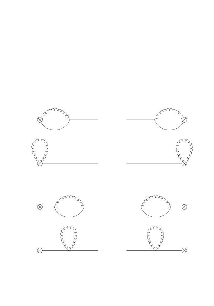
Just as we have contact terms in the fermion propagator, we should expect to see $O(a)$ contact terms arising in eq. (55) when $x=y$ or $x^{\prime}=y^{\prime}$. These will give rise to a “contact Green’s function”, $C^{\mathcal{O}}$, which will have to be subtracted from the operator Green’s function, just as we subtracted a $\delta$ function from the fermion propagator. This contact term is thus given by

$$C^{\mathcal{O}}(p,m) = \frac{1}{V}\sum_{x,x^{\prime}}e^{-{\rm i}p\cdot(x-x^{\prime})}\left\langle\Big{[}M^{-1}O+OM^{-1}\Big{]}_{x,x^{\prime}}\right\rangle_{A}$$ (57)

$$\equiv \;{\mathcal{F}}\;\left\langle M^{-1}O+OM^{-1}\right\rangle_{A}.$$

Since the coefficient of $C^{\mathcal{O}}$ will be $O(a)$, we only need to calculate it for the unimproved operator $\bar{\psi}O\psi$, and we only need the leading order in $a$. The Feynman diagrams needed to calculate $C^{\mathcal{O}}$ to $O(g^{2})$ are shown in Fig. 1. There is no extra calculation involved. All the graphs needed already occur in the perturbative expansion of the operator and propagator.

Figure 1: The one-loop lattice Feynman diagrams needed for the contact Green’s function $C_{\mathcal{O}}(p,m)$, defined in eq. (57).

Finding the contact Green’s function is simple when we consider point operators of the type $\bar{\psi}\Gamma_{i}\psi$ where $\Gamma_{i}$ is any $4\times 4$ matrix. Because there are no covariant derivatives in the operator, it is unaffected by the averaging over gauge fields, and eq. (57) simplifies to give

$$C^{\Gamma_{i}}(p,m)=\Gamma_{i}S(p,m)+S(p,m)\Gamma_{i}=\left\{\Gamma_{i}\,,\,S(p,m)\right\}\;.$$ (58)

The contact Green’s function are more complicated in the general case. Their expressions for the one-link operators are given in the Appendix (Sects. (A.6) to (A.9)).

So, by subtracting a contact term proportional to $C^{\mathcal{O}}(p,m)$ in a Green’s function and by choosing appropriately the improvement coefficients, an improved Green’s function can be obtained. The resulting expression for a renormalised improved off-shell Green’s function is:

$$G_{R}^{\mathcal{O}}(p,m_{R};\mu^{2}) = \frac{Z_{\mathcal{O}}(\mu^{2};c_{1},\cdots,c_{n})}{Z_{2}(\mu^{2})\,(1+amb_{\psi})}$$

$$\times\Big{[}G^{\cal O^{\rm imp}}(p,m;c_{0},c_{1},\cdots,c_{n})-\frac{a}{2}\lambda_{\mathcal{O}}C^{\mathcal{O}}(p,m)\Big{]}.$$

The factor $1/[Z_{2}(\mu^{2})(1+amb_{\psi})]$ accounts for the wave-function renormalisation. The Green’s function in eq. (55) depends linearly on the $c_{k}$ coefficients, while the renormalised Green’s function is independent of the $c_{k}$s. From this we can deduce that $1/Z_{\mathcal{O}}(\mu^{2};c_{1},\cdots,c_{n})$ must depend linearly on $c_{k}$ too, so we can write

$$Z_{\mathcal{O}}(\mu^{2};c_{1},\cdots,c_{n})=\frac{Z_{\mathcal{O}}(\mu^{2};0,\cdots,0)}{1+\sum_{k=1}^{n}\zeta_{k}c_{k}},$$ (60)

where the $\zeta$s are coefficients depending on $g^{2}$. At the one-loop level, using the fact that $Z=1+O(g^{2})$ and that the $\zeta$s are $O(g^{2})$, we can write

$$Z_{\mathcal{O}}(\mu^{2};c_{1},\cdots,c_{n})=Z_{\mathcal{O}}(\mu^{2};0,\cdots,0)-\sum_{k=1}^{n}\zeta_{k}c_{k}+O(g^{4})\,.$$ (61)

Our final formula for the renormalised and improved Green’s function is

$$G_{R}^{\mathcal{O}}(p,m_{R};\mu^{2}) = \frac{1}{Z_{2}(\mu^{2})\,(1+amb_{\psi})}\frac{Z_{\mathcal{O}}(\mu^{2};0,\cdots,0)}{1+\sum_{k}\zeta_{k}c_{k}}$$ (62)

$$\times\left[G^{{\mathcal{O}}^{\rm imp}}(p,m;c_{0},c_{1},\cdots,c_{n})-\frac{a}{2}\lambda_{\mathcal{O}}C^{\mathcal{O}}(p,m)\right].$$

The improvement coefficients $b,c,\lambda$ and $\zeta$ are independent of the renormalisation scheme, while the renormalisation constants $Z$ are in general scheme dependent. Therefore it can be useful to split the renormalisation and improvement into two stages, and to define “improved bare” Green’s functions by

$$G_{\star}^{\mathcal{O}}(p,m_{\star}) = \frac{1}{1+amb_{\psi}}\;\frac{1}{1+\sum_{k}\zeta_{k}c_{k}}$$

$$\times\left[G^{{\mathcal{O}}^{\rm imp}}(p,m;c_{0},c_{1},\cdots,c_{n})-\frac{a}{2}\lambda_{\mathcal{O}}C^{\mathcal{O}}(p,m)\right]\,,$$

where $m_{\star}=m(1+amb_{m})$, using the same value for $b_{m}$ as found from the fermion propagator (eq. (41)). As in the propagator section, we will use the suffix $\star$ to denote bare quantities which have been improved to $O(a)$.

The second step is then to renormalise this improved Green’s function multiplicatively,

$$G_{R}^{\mathcal{O}}(p,m_{R};\mu^{2})=\frac{Z_{\mathcal{O}}(\mu^{2};0,\cdots,0)}{Z_{2}(\mu^{2})}G_{\star}^{\mathcal{O}}(p,m_{\star}).$$ (64)

Figure 2: The one-loop lattice Feynman diagrams needed for the amputated Green’s function (vertex function), $\Lambda^{{\mathcal{O}}^{\rm imp}}(p,m;c_{0},c_{1},\cdots,c_{n})$, as defined in eq. (65).

It is useful to write corresponding equations for amputated Green’s functions too. We define the amputated Green’s function $\Lambda$ in the standard way:

$$\Lambda^{{\mathcal{O}}^{\rm imp}}(p,m;c_{0},c_{1},\cdots,c_{n})\equiv S^{-1}(p,m)G^{{\mathcal{O}}^{\rm imp}}(p,m;c_{0},c_{1},\cdots,c_{n})S^{-1}(p,m),$$ (65)

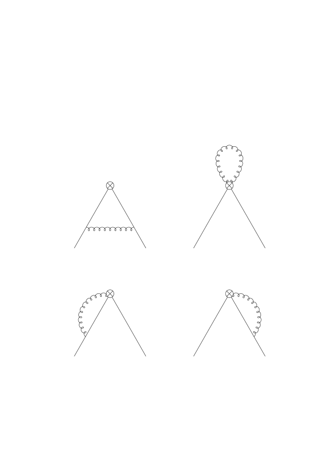
where $S(p,m)$ is the full fermion propagator. The amputation of eq. (65) removes all fermion self-energy diagrams from the perturbative expansion of $\Lambda$. The one-loop Feynman diagrams for $\Lambda$ are shown in Fig. 2.

The improved amputated Green’s function, $\Lambda_{\star}$, is naturally defined by

$$\Lambda^{\mathcal{O}}_{\star}(p,m_{\star})\equiv S_{\star}^{-1}(p,m_{\star})G^{\mathcal{O}}_{\star}(p,m_{\star})S_{\star}^{-1}(p,m_{\star}).$$ (66)

From eq. (64) we obtain the renormalised amputated Green’s function:

$$\Lambda_{R}^{\mathcal{O}}(p,m_{R};\mu^{2})=Z_{2}(\mu^{2})Z_{\mathcal{O}}(\mu^{2};0,\cdots,0)\Lambda_{\star}^{\mathcal{O}}(p,m_{\star}).$$ (67)

Substituting eq. (29) and eq. (4.1) and using eq. (65) we find

$$\Lambda_{\star}^{\mathcal{O}}(p,m_{\star}) = \frac{1+amb_{\psi}}{1+\sum_{k}\zeta_{k}c_{k}}\Big{[}\Lambda^{{\mathcal{O}}^{\rm imp}}(p,m;c_{0},c_{1},\cdots,c_{n})$$ (68)

$$-\frac{a}{2}\lambda_{\mathcal{O}}S^{-1}(p,m)C^{\mathcal{O}}(p,m)S^{-1}(p,m)$$

$$+\frac{a}{2}\lambda_{\psi}\left\{S^{-1}(p,m),\Lambda^{{\mathcal{O}}^{\rm imp}}(p,m;c_{0},c_{1},\cdots,c_{n})\right\}\Big{]}\;.$$

Similarly to what was done in the case of the propagator, one can now expand $\Lambda^{\mathcal{O}}$, $S^{-1}$ and $C^{\mathcal{O}}$ in powers of $a$ and thus obtain a non-linear condition analogous to eq. (27), from which the improvement coefficients can be derived. In the case of the local operators $\bar{\psi}\Gamma_{i}\psi$, the expression eq. (58) for the contact term means that we can write the expression for $\Lambda_{\star}$ in the simpler form

$$\Lambda_{\star}^{\Gamma_{i}}(p,m_{\star})=\frac{1+amb_{\psi}}{1+\zeta_{1}^{\Gamma_{i}}c_{1}^{\Gamma_{i}}}\Big{[}\Lambda^{\Gamma_{i}^{\rm imp}}(p,m;c_{0},c_{1})$$ (69)

$$-\frac{a}{2}\lambda_{\Gamma_{i}}\left\{S^{-1}(p,m),\Gamma_{i}\right\}+\frac{a}{2}\lambda_{\psi}\left\{S^{-1}(p,m),\Lambda^{\Gamma_{i}^{\rm imp}}(p,m;c_{0},c_{1})\right\}\Big{]}\,.$$

From eq. (68) we can see that the two improvement coefficients $\lambda_{\psi}$ and $\lambda_{\mathcal{O}}$ associated with the contact terms are only needed for off-shell improvement, because the inverse propagator $S^{-1}(p,m)$ vanishes on-shell.

4.2 Results for point quark operators

We shall now calculate the matrix elements of all point operators up to $O(g^{2}a)$ including the finite terms. This goes beyond the work of Heatlie et al. [7], who only considered the $g^{2}a\ln a$ terms. Including all $O(g^{2}a)$ terms will enable us to compute the improvement coefficients to $O(g^{2})$.

The calculations are carried out for arbitrary $m^{2}/p^{2}$, not just for $m^{2}\ll p^{2}$ as in our previous papers [16, 18, 19]. We give the results for the amputated Green’s functions.

In this section we show how the improvement coefficients and renormalisation constants are calculated in one particular case, that of the scalar operator

$$\left({\mathcal{O}}^{S}\right)^{\rm imp}=\left(\bar{\psi}\psi\right)^{\rm imp}=(1+a\,m\,c_{0})\bar{\psi}\psi-\frac{1}{2}ac_{1}\bar{\psi}\not{{\mbox{\parbox[b]{0.0pt}{$D$}\raisebox{7.3194pt}{${\,\scriptstyle{\leftrightarrow}}$}}}}\psi.$$ (70)

The Green’s functions and results for the other operators are given in the Appendix. We consider forward matrix elements, therefore we drop the total derivative terms in the improved bases (although in the scalar case this does not make any difference), which now all have the form

$${\mathcal{O}}_{\Gamma}^{\rm imp}=\bar{\psi}\Gamma\psi-\frac{1}{4}ac_{1}^{\Gamma}\bar{\psi}\{\not{{\mbox{\parbox[b]{0.0pt}{$D$}\raisebox{7.3194pt}{${\,\scriptstyle{\leftrightarrow}}$}}}},\Gamma\}\psi+amc_{0}^{\Gamma}\bar{\psi}\Gamma\psi.$$ (71)

The one-loop expression for the amputated scalar Green’s function up to $O(a)$ is:

$$\Lambda^{S}(p,m;0,c_{1}^{S})=1-a\,{\rm i}{\not{p}}\,c_{1}^{S}$$

$$+ \frac{g^{2}C_{F}}{16\,\pi^{2}}\;\,\Big{[}-11.06803+2\,\alpha+9.98679\,c_{\scriptscriptstyle{SW}}+0.01689\,{\,c_{\scriptscriptstyle{SW}}^{2}}$$

$$+\,c_{1}^{S}(-19.17181+13.80068\,c_{\scriptscriptstyle{SW}}-3.53833\,{\,c_{\scriptscriptstyle{SW}}^{2}})$$

$$-(3+\alpha)\,L(ap,am)-3\,(3+\alpha)\,\,T\left(p^{2}/m^{2}\right)\Big{]}$$

$$+ {\rm i}{\not{p}}\,\frac{g^{2}C_{F}}{16\,\pi^{2}}\;\,4\,\alpha\,\frac{m}{p^{2}}\,\Big{[}-1+\,T\left(p^{2}/m^{2}\right)\Big{]}$$

$$+ a\,{\rm i}{\not{p}}\,\frac{g^{2}C_{F}}{16\,\pi^{2}}\;\Big{[}6.34664-0.14375\,\alpha+1.48503\,c_{\scriptscriptstyle{SW}}-1.28605\,{\,c_{\scriptscriptstyle{SW}}^{2}}$$

$$+c_{1}^{S}(11.65102-\alpha-1.41422\,c_{\scriptscriptstyle{SW}}+0.78465\,{\,c_{\scriptscriptstyle{SW}}^{2}})$$

$$+({\frac{3}{2}}+\alpha+\alpha\,c_{1}^{S}+{\frac{3}{2}\,c_{\scriptscriptstyle{SW}}})\,L(ap,am)$$

$$+3\,\left(\alpha+3\,c_{\scriptscriptstyle{SW}}\right)\,T\left(p^{2}/m^{2}\right)-4\,\alpha\,\frac{m^{2}}{m^{2}+p^{2}}$$

$$+\left(\frac{15}{2}+10\,\alpha-3\,\alpha\,c_{1}^{S}-\frac{15}{2}\,c_{\scriptscriptstyle{SW}}\right)\,\frac{m^{2}}{p^{2}}\left(1-\,T\left(p^{2}/m^{2}\right)\right)\Big{]}$$

$$+ a\,m\,\frac{g^{2}C_{F}}{16\,\pi^{2}}\;\Big{[}31.06826-4.14375\,\alpha-33.97148\,c_{\scriptscriptstyle{SW}}+3.04688\,{\,c_{\scriptscriptstyle{SW}}^{2}}$$

$$+c_{1}^{S}(-6.08204+2.20074\,c_{\scriptscriptstyle{SW}}+1.44647\,{\,c_{\scriptscriptstyle{SW}}^{2}})$$

$$+(9+\alpha-6\,c_{\scriptscriptstyle{SW}})\,L(ap,am)-2\,(3+\alpha)\,\frac{m^{2}}{m^{2}+p^{2}}$$

$$+2\,(12+5\,\alpha-3\,c_{1}^{S}-\alpha\,c_{1}^{S}-3\,c_{\scriptscriptstyle{SW}})\,\,T\left(p^{2}/m^{2}\right)\Big{]}.$$

We only need to give the expression for $\Lambda^{S}$ when $c_{0}=0$, since the full expression with non-zero $c_{0}$ can be recovered by using eq. (56).

To improve the Green’s functions, we need to choose the improvement coefficients so that all $O(a)$ terms in the expressions eq. (4.1) or eq. (68) vanish. It is not immediately obvious that this will be possible, because there are many more $O(a)$ terms than there are improvement coefficients, and therefore more equations to be satisfied than there are unknowns. For general $\,c_{\scriptscriptstyle{SW}}$ we can not satisfy all the equations, we can only remove all $O(a)$ effects if $\,c_{\scriptscriptstyle{SW}}=1+O(g^{2})$. In this case we can derive perturbative expressions for the improvement coefficients. The results are

$$c_{0}^{S} = 1-c_{1}^{S}+\frac{g^{2}C_{F}}{16\,\pi^{2}}\;(22.79406-8.45146c_{1}^{S}),$$

$$\lambda_{S} = 1-c_{1}^{S}+\frac{g^{2}C_{F}}{16\,\pi^{2}}\;(16.39210-10.88629c_{1}^{S}),$$

$$\zeta_{1}^{S} = -\frac{g^{2}C_{F}}{16\,\pi^{2}}\;8.90946.$$ (73)

All three improvement coefficients are gauge invariant. There is one free parameter in this system of equations. The improvement coefficient $c_{1}^{S}$ can take any value, but once it is chosen, the values of the other improvement coefficients are fixed. This freedom comes from an equation of motion, which allows us to compensate for a change in one of the improvement coefficients by adjusting the other two coefficients. For example, there is a particularly interesting value of $c_{1}^{S}$ where $\lambda_{S}$ vanishes, which means that the scalar three-point function contains no contact terms, and so even off-shell it is simply renormalised by a multiplicative factor. This value of $c_{1}^{S}$ is

$${\tilde{c}}_{1}^{S}=1+\frac{g^{2}C_{F}}{16\,\pi^{2}}\;5.50582+O(g^{4}).$$ (74)

The improvement coefficients $c_{0}^{S}$ and $\lambda_{S}$ are only defined at $\,c_{\scriptscriptstyle{SW}}=1$, but $\zeta_{1}^{S}$ can also be defined for general $\,c_{\scriptscriptstyle{SW}}$ values. The result is

$$\zeta_{1}^{S}=\frac{g^{2}C_{F}}{16\,\pi^{2}}\;(-19.17181+13.80068\,c_{\scriptscriptstyle{SW}}-3.53833\,c_{\scriptscriptstyle{SW}}^{2}).$$ (75)

All these results are gauge invariant.

	$Z^{\scriptscriptstyle{\overline{{\rm MS}}}}(\mu^{2};0)$
$S$	$1+\frac{g^{2}C_{F}}{16\,\pi^{2}}\;(-12.95241-7.73792\,c_{\scriptscriptstyle{SW}}+1.38038\,c_{\scriptscriptstyle{SW}}^{2}+6\ln a\mu)$
$P$	$1+\frac{g^{2}C_{F}}{16\,\pi^{2}}\;(-22.59544+2.24887\,c_{\scriptscriptstyle{SW}}-2.03602\,c_{\scriptscriptstyle{SW}}^{2}+6\ln a\mu)$
$V$	$1+\frac{g^{2}C_{F}}{16\,\pi^{2}}\;(-20.61780+4.74556\,c_{\scriptscriptstyle{SW}}+0.54317\,c_{\scriptscriptstyle{SW}}^{2})$
$A$	$1+\frac{g^{2}C_{F}}{16\,\pi^{2}}\;(-15.79628-0.24783\,c_{\scriptscriptstyle{SW}}+2.25137\,c_{\scriptscriptstyle{SW}}^{2})$
$H$	$1+\frac{g^{2}C_{F}}{16\,\pi^{2}}\;(-17.01808+3.91333\,c_{\scriptscriptstyle{SW}}+1.97230\,c_{\scriptscriptstyle{SW}}^{2}-2\ln a\mu)$

Table 2: The renormalisation constants $Z^{\scriptscriptstyle{\overline{{\rm MS}}}}$ for the point operators (with no improvement term added, i.e. $c_{1}^{\Gamma}=0$).

	$\zeta_{1}^{\Gamma}$
$S$	$\frac{g^{2}C_{F}}{16\,\pi^{2}}\;(-19.17181+13.80068\,c_{\scriptscriptstyle{SW}}-3.53833\,c_{\scriptscriptstyle{SW}}^{2})$
$V$	$\frac{g^{2}C_{F}}{16\,\pi^{2}}\;(-9.78635+3.41640\,c_{\scriptscriptstyle{SW}}+0.88458\,c_{\scriptscriptstyle{SW}}^{2})$
$A$	$\frac{g^{2}C_{F}}{16\,\pi^{2}}\;(-19.37225+10.31673\,c_{\scriptscriptstyle{SW}}-0.88458\,c_{\scriptscriptstyle{SW}}^{2})$
$H$	$\frac{g^{2}C_{F}}{16\,\pi^{2}}\;(-16.24376+6.85531\,c_{\scriptscriptstyle{SW}}+0.58972\,c_{\scriptscriptstyle{SW}}^{2})$

Table 3: The improvement coefficients $\zeta_{1}^{\Gamma}$. These give the renormalisation constants when $c_{1}^{\Gamma}$ is non-zero, see eq. (61).

	$c_{0}^{\Gamma}$
$S$	$1-c_{1}^{S}+\frac{g^{2}C_{F}}{16\,\pi^{2}}\;(22.79406-8.45146\,c_{1}^{S})$
$V$	$1-c_{1}^{V}+\frac{g^{2}C_{F}}{16\,\pi^{2}}\;(18.14912-6.96476\,c_{1}^{V})$
$A$	$1-c_{1}^{A}+\frac{g^{2}C_{F}}{16\,\pi^{2}}\;(18.02539-13.36028\,c_{1}^{A})$
$H$	$1-\,c_{1}^{H}+\frac{g^{2}C_{F}}{16\,\pi^{2}}\;(16.47708-12.86471\,\,c_{1}^{H})$

Table 4: The improvement coefficients $c_{0}^{\Gamma}$ for general $c_{1}^{\Gamma}$ at $\,c_{\scriptscriptstyle{SW}}=1$.

	$\lambda_{\Gamma}$
$S$	$1-c_{1}^{S}+\frac{g^{2}C_{F}}{16\,\pi^{2}}\;(16.39210-10.88629\,c_{1}^{S})$
$V$	$1-c_{1}^{V}+\frac{g^{2}C_{F}}{16\,\pi^{2}}\;(13.71395-2.29988\,c_{1}^{V})$
$A$	$1-c_{1}^{A}+\frac{g^{2}C_{F}}{16\,\pi^{2}}\;(11.46014-8.37649\,c_{1}^{A})$
$H$	$1-\,c_{1}^{H}+\frac{g^{2}C_{F}}{16\,\pi^{2}}\;(10.56742-5.51435\,\,c_{1}^{H})$

Table 5: The improvement coefficients $\lambda_{\Gamma}$ for general $c_{1}^{\Gamma}$ at $\,c_{\scriptscriptstyle{SW}}=1$.

	${\tilde{c}}_{0}^{\Gamma}$	${\tilde{c}}_{1}^{\Gamma}$
$S$	$\frac{g^{2}C_{F}}{16\,\pi^{2}}\;\,8.83678$	$1+\frac{g^{2}C_{F}}{16\,\pi^{2}}\;\,5.50582$
$P$	$-\frac{g^{2}C_{F}}{16\,\pi^{2}}\;\,5.21443$	–
$V$	$-\frac{g^{2}C_{F}}{16\,\pi^{2}}\;\,0.22971$	$1+\frac{g^{2}C_{F}}{16\,\pi^{2}}\;\,11.41407$
$A$	$\frac{g^{2}C_{F}}{16\,\pi^{2}}\;\,1.58146$	$1+\frac{g^{2}C_{F}}{16\,\pi^{2}}\;\,3.08365$
$H$	$-\frac{g^{2}C_{F}}{16\,\pi^{2}}\;\,1.44071$	$1+\frac{g^{2}C_{F}}{16\,\pi^{2}}\;\,5.05307$

Table 6: The improvement coefficients $c_{0}^{\Gamma}$ and $c_{1}^{\Gamma}$ when the contact term $\lambda_{\Gamma}$ is chosen to be zero.

We calculate the continuum Green’s functions (needed for the $Z^{\scriptscriptstyle{\overline{{\rm MS}}}}$ factors) in the ${\overline{{\rm MS}}}$ (minimal subtraction) scheme. In this paper we use a totally anticommuting $\gamma_{5}$, even when $d\neq 4$. For the scalar Green’s function the result in the ${\overline{{\rm MS}}}$ scheme is

$$\Lambda^{S}_{\scriptscriptstyle{\overline{{\rm MS}}}}(p,m_{\scriptscriptstyle{\overline{{\rm MS}}}}) = 1+\frac{g^{2}C_{F}}{16\,\pi^{2}}\;\,\Big{[}4+2\,\alpha-(3+\alpha)\,\ln\left(\frac{p^{2}+m_{\scriptscriptstyle{\overline{{\rm MS}}}}^{2}}{\mu^{2}}\right)$$ (76)

$$\qquad\qquad-3\,(3+\alpha)\,T\left(p^{2}/m_{\scriptscriptstyle{\overline{{\rm MS}}}}^{2}\right)\Big{]}$$

$$+ {\rm i}\frac{m_{\scriptscriptstyle{\overline{{\rm MS}}}}\,{\not{p}}}{p^{2}}\,\frac{g^{2}C_{F}}{16\,\pi^{2}}\;\,4\,\alpha\,\left[-1+T\left(p^{2}/m_{\scriptscriptstyle{\overline{{\rm MS}}}}^{2}\right)\right].$$

We can now calculate $Z^{\scriptscriptstyle{\overline{{\rm MS}}}}$ which is defined by

$$Z_{2}^{\scriptscriptstyle{\overline{{\rm MS}}}}(\mu^{2})Z_{S}^{\scriptscriptstyle{\overline{{\rm MS}}}}(\mu^{2};c_{1}^{S})\Lambda_{S}(p,m;0,c_{1}^{S})=\Lambda^{\scriptscriptstyle{\overline{{\rm MS}}}}_{S}(p,m_{\scriptscriptstyle{\overline{{\rm MS}}}})\,.$$ (77)

The result is

$$Z_{S}^{\scriptscriptstyle{\overline{{\rm MS}}}}(\mu^{2};c_{1}^{S}) = \frac{1+\frac{g^{2}C_{F}}{16\,\pi^{2}}\;(-12.95241-7.73792\,c_{\scriptscriptstyle{SW}}+1.38038\,c_{\scriptscriptstyle{SW}}^{2}+6\ln a\mu)}{1+\frac{g^{2}C_{F}}{16\,\pi^{2}}\;(-19.17181+13.80068\,c_{\scriptscriptstyle{SW}}-3.53833\,c_{\scriptscriptstyle{SW}}^{2})c_{1}^{S}}$$ (78)

$$= \frac{Z_{S}^{\scriptscriptstyle{\overline{{\rm MS}}}}(\mu^{2};0)}{1+\zeta_{1}^{S}c_{1}^{S}}\;.$$

In the MOM scheme we define the $Z$ for an operator ${\cal O}$ by

$$Z^{\rm MOM}_{2}(M^{2})Z^{\rm MOM}_{\cal O}(M^{2}){\rm Tr}\left[(\Lambda^{\rm Born}_{\cal O}(p))^{\dagger}\Lambda_{\cal O}(p)\right]={\rm Tr}\left[(\Lambda^{\rm Born}_{\cal O}(p))^{\dagger}\Lambda^{\rm Born}_{\cal O}(p)\right]$$ (79)

when $p^{2}=M^{2}$, where $\Lambda^{\rm Born}_{\cal O}$ is the operator’s Born term. Applying this definition to the scalar operator gives

$$Z^{\rm MOM}_{2}(M^{2})Z^{\rm MOM}_{S}(M^{2};0)=\frac{4N_{c}}{{\rm Tr}\left[\Lambda^{S}(p,m;0,0)\right]}$$ (80)

at $p^{2}=M^{2}$, so

$$Z^{\rm MOM}_{S}(M^{2};0)=1 + \frac{g^{2}C_{F}}{16\,\pi^{2}}\;\Big{[}-5.57638-7.73792\,c_{\scriptscriptstyle{SW}}+1.38038\,c_{\scriptscriptstyle{SW}}^{2}$$ (81)

$$-\alpha+3\,L\left(aM,am_{\star}\right)+3\,(3+\alpha)\,T\left(M^{2}/m_{\star}^{2}\right)$$

$$-\alpha\,\frac{m_{\star}^{2}}{M^{2}}\left(1-T\left(M^{2}/m_{\star}^{2}\right)\right)\Big{]}+O(a).$$

The same procedure can be repeated for all the local operators. In Tables 2-6 we give the improvement coefficients and ${\overline{{\rm MS}}}$ renormalisation constants for all point operators. The ${\overline{{\rm MS}}}$ renormalisation constants are defined by equations analogous to eq. (77). The lattice $\Lambda$s and ${\overline{{\rm MS}}}$-scheme $\Lambda$s are all given in the Appendix. In several of the tables there is no entry for the pseudoscalar operator – this is because it has no $c_{1}$ improvement term, so the associated quantities are not defined. The $Z$s in the MOM scheme are given in the Appendix.

The $c_{0}^{\Gamma}$ values in table 4 agree with the values given in [20] for the case $c_{1}^{\Gamma}\equiv 0$.

4.3 Results for one-link quark operators

We consider now the operators in eq. (7). We study the improvement of these operators along the same lines used for the point operators. The expressions for the contact Green’s functions (57) will be more complicated, and are given in the Appendix.

From eqs. (15), (2) and (17), we can see that in forward matrix elements a basis for the improvement is given in the unpolarised case (${\mathcal{O}}_{\mu\nu},\tau_{3}^{(6)}$ and ${\mathcal{O}}_{\mu\nu},\tau_{1}^{(3)}$) by

$$\left({\mathcal{O}}_{\mu\nu}\right)^{\rm imp} = \frac{1}{2}\left(1+a\,m\,c_{0}\right)\bar{\psi}\gamma_{\mu}\mbox{\parbox[b]{0.0pt}{$D$}\raisebox{7.3194pt}{${\,\scriptstyle{\leftrightarrow}}$}}_{\nu}\psi+\frac{1}{8}\,a\,{\rm i}c_{1}\sum_{\lambda}\bar{\psi}\sigma_{\mu\lambda}\left[\mbox{\parbox[b]{0.0pt}{$D$}\raisebox{7.3194pt}{${\,\scriptstyle{\leftrightarrow}}$}}_{\nu},\mbox{\parbox[b]{0.0pt}{$D$}\raisebox{7.3194pt}{${\,\scriptstyle{\leftrightarrow}}$}}_{\lambda}\right]\psi$$ (82)

$$-\frac{1}{8}\,a\,c_{2}\bar{\psi}\left\{\mbox{\parbox[b]{0.0pt}{$D$}\raisebox{7.3194pt}{${\,\scriptstyle{\leftrightarrow}}$}}_{\mu},\mbox{\parbox[b]{0.0pt}{$D$}\raisebox{7.3194pt}{${\,\scriptstyle{\leftrightarrow}}$}}_{\nu}\right\}\psi,$$

in the polarised case with $\mu\neq\nu$ (${\mathcal{O}}_{\mu\nu}^{5},\tau_{4}^{(6)}$) by

$$\left({\mathcal{O}}_{\mu\nu}^{5}\right)^{\rm imp} = \frac{1}{2}\left(1+a\,m\,c_{0}\right)\bar{\psi}\gamma_{\mu}\gamma_{5}\mbox{\parbox[b]{0.0pt}{$D$}\raisebox{7.3194pt}{${\,\scriptstyle{\leftrightarrow}}$}}_{\nu}\psi-\frac{1}{4}\,{\rm i}a\,c_{1}\,\bar{\psi}\sigma_{\mu\nu}\mbox{\parbox[b]{0.0pt}{$D$}\raisebox{7.3194pt}{${\,\scriptstyle{\leftrightarrow}}$}}_{\nu}^{2}\psi$$ (83)

$$-\frac{1}{8}\,a\,{\rm i}\,c_{2}\,\sum_{\lambda\neq\mu,\nu}\bar{\psi}\sigma_{\mu\lambda}\gamma_{5}\left\{\mbox{\parbox[b]{0.0pt}{$D$}\raisebox{7.3194pt}{${\,\scriptstyle{\leftrightarrow}}$}}_{\lambda},\mbox{\parbox[b]{0.0pt}{$D$}\raisebox{7.3194pt}{${\,\scriptstyle{\leftrightarrow}}$}}_{\nu}\right\}\psi,$$

and in the polarised case when $\mu=\nu$ (${\mathcal{O}}_{\mu\nu}^{5},\tau_{4}^{(3)}$) by

$$\left({\mathcal{O}}_{\mu\nu}^{5}\right)^{\rm imp} = \frac{1}{2}\left(1+a\,m\,c_{0}\right)\bar{\psi}\gamma_{\mu}\gamma_{5}\mbox{\parbox[b]{0.0pt}{$D$}\raisebox{7.3194pt}{${\,\scriptstyle{\leftrightarrow}}$}}_{\nu}\psi-\frac{1}{8}\,a\,{\rm i}\,c_{1}\,\bar{\psi}\sigma_{\mu\lambda}\gamma_{5}\left\{\mbox{\parbox[b]{0.0pt}{$D$}\raisebox{7.3194pt}{${\,\scriptstyle{\leftrightarrow}}$}}_{\lambda},\mbox{\parbox[b]{0.0pt}{$D$}\raisebox{7.3194pt}{${\,\scriptstyle{\leftrightarrow}}$}}_{\nu}\right\}\psi.$$ (84)

	$Z^{\scriptscriptstyle{\overline{{\rm MS}}}}(\mu^{2};0,0)$
${\mathcal{O}}_{\mu\nu},\tau_{3}^{(6)}$	$1+\frac{g^{2}C_{F}}{16\,\pi^{2}}\;(-1.27959+3.87297\;\,c_{\scriptscriptstyle{SW}}+0.67826\;\,c_{\scriptscriptstyle{SW}}^{2}-\frac{16}{3}\ln a\mu)$
${\mathcal{O}}_{\mu\nu},\tau_{1}^{(3)}$	$1+\frac{g^{2}C_{F}}{16\,\pi^{2}}\;(-2.56184+3.96980\;\,c_{\scriptscriptstyle{SW}}+1.03973\;\,c_{\scriptscriptstyle{SW}}^{2}-\frac{16}{3}\ln a\mu)$
${\mathcal{O}}_{\mu\nu}^{5},\tau_{4}^{(6)}$	$1+\frac{g^{2}C_{F}}{16\,\pi^{2}}\;(-0.34512+1.35931\;\,c_{\scriptscriptstyle{SW}}+1.89255\;\,c_{\scriptscriptstyle{SW}}^{2}-\frac{16}{3}\ln a\mu)$
${\mathcal{O}}_{\mu\nu}^{5},\tau_{4}^{(3)}$	$1+\frac{g^{2}C_{F}}{16\,\pi^{2}}\;(-0.16738+1.24953\;\,c_{\scriptscriptstyle{SW}}+1.99804\;\,c_{\scriptscriptstyle{SW}}^{2}-\frac{16}{3}\ln a\mu)$

Table 7: The ${\overline{{\rm MS}}}$-scheme renormalisation constants for the one-link operators.

	$\zeta_{1}$
${\mathcal{O}}_{\mu\nu},\tau_{3}^{(6)}$	$\frac{g^{2}C_{F}}{16\,\pi^{2}}\;(-4.27417+1.08793\,c_{\scriptscriptstyle{SW}})$
${\mathcal{O}}_{\mu\nu},\tau_{1}^{(3)}$	$\frac{g^{2}C_{F}}{16\,\pi^{2}}\;(-4.27417+1.08793\,c_{\scriptscriptstyle{SW}})$
${\mathcal{O}}_{\mu\nu}^{5},\tau_{4}^{(6)}$	$\frac{g^{2}C_{F}}{16\,\pi^{2}}\;(-5.61603+4.10778\,c_{\scriptscriptstyle{SW}}-0.26315\,c_{\scriptscriptstyle{SW}}^{2})$
${\mathcal{O}}_{\mu\nu}^{5},\tau_{4}^{(3)}$	$\frac{g^{2}C_{F}}{16\,\pi^{2}}\;(-15.31376+8.54773\;\,c_{\scriptscriptstyle{SW}}-0.26036\;\,c_{\scriptscriptstyle{SW}}^{2})$

Table 8: The improvement coefficients $\zeta_{1}$ for the one-link operators.

	$\zeta_{2}$
${\mathcal{O}}_{\mu\nu},\tau_{3}^{(6)}$	$\frac{g^{2}C_{F}}{16\,\pi^{2}}\;(-9.40584+4.60327\;\,c_{\scriptscriptstyle{SW}}+0.46669\;\,c_{\scriptscriptstyle{SW}}^{2})$
${\mathcal{O}}_{\mu\nu},\tau_{1}^{(3)}$	$\frac{g^{2}C_{F}}{16\,\pi^{2}}\;(-6.67330+4.53710\;\,c_{\scriptscriptstyle{SW}}+0.44621\;\,c_{\scriptscriptstyle{SW}}^{2})$
${\mathcal{O}}_{\mu\nu}^{5},\tau_{4}^{(6)}$	$\frac{g^{2}C_{F}}{16\,\pi^{2}}\;(-8.29791+4.21724\;\,c_{\scriptscriptstyle{SW}}-0.49384\;\,c_{\scriptscriptstyle{SW}}^{2})$
${\mathcal{O}}_{\mu\nu}^{5},\tau_{4}^{(3)}$	$-$

Table 9: The improvement coefficients $\zeta_{2}$ for the one-link operators.

	$c_{0}$
${\mathcal{O}}_{\mu\nu},\tau_{3}^{(6)}$	$1-c_{2}+\frac{g^{2}C_{F}}{16\,\pi^{2}}\;(16.34500-12.24534\,c_{2})$
${\mathcal{O}}_{\mu\nu},\tau_{1}^{(3)}$	$1-c_{2}+\frac{g^{2}C_{F}}{16\,\pi^{2}}\;(17.20377-8.69045\,c_{2})$
${\mathcal{O}}_{\mu\nu}^{5},\tau_{4}^{(6)}$	$1-c_{2}+\frac{g^{2}C_{F}}{16\,\pi^{2}}\;(16.28373-10.73103\,c_{2})$
${\mathcal{O}}_{\mu\nu}^{5},\tau_{4}^{(3)}$	$1-c_{1}+\frac{g^{2}C_{F}}{16\,\pi^{2}}\;(16.95724-11.33434\,c_{1})$

Table 10: The improvement coefficients $c_{0}$ for general $c_{2}$ at $\,c_{\scriptscriptstyle{SW}}=1$ for the one-link operators.

	$c_{1}$
${\mathcal{O}}_{\mu\nu},\tau_{3}^{(6)}$	$c_{2}+O(g^{2})$
${\mathcal{O}}_{\mu\nu},\tau_{1}^{(3)}$	$c_{2}+O(g^{2})$
${\mathcal{O}}_{\mu\nu}^{5},\tau_{4}^{(6)}$	$c_{2}+\frac{g^{2}C_{F}}{16\,\pi^{2}}\;(1.18321+0.84682\,c_{2})$
${\mathcal{O}}_{\mu\nu}^{5},\tau_{4}^{(3)}$	$-$

Table 11: The improvement coefficients $c_{1}$ for general $c_{2}$ at $\,c_{\scriptscriptstyle{SW}}=1$ for the one-link operators.

	$\lambda_{\mathcal{O}}$
${\mathcal{O}}_{\mu\nu},\tau_{3}^{(6)}$	$1-c_{2}+\frac{g^{2}C_{F}}{16\,\pi^{2}}\;(8.13135-3.04784\,c_{2})$
${\mathcal{O}}_{\mu\nu},\tau_{1}^{(3)}$	$1-c_{2}+\frac{g^{2}C_{F}}{16\,\pi^{2}}\;(9.28735-0.52613\,c_{2})$
${\mathcal{O}}_{\mu\nu}^{5},\tau_{4}^{(6)}$	$1-c_{2}+\frac{g^{2}C_{F}}{16\,\pi^{2}}\;(8.48845-1.84428\,c_{2})$
${\mathcal{O}}_{\mu\nu}^{5},\tau_{4}^{(3)}$	$1-c_{1}+\frac{g^{2}C_{F}}{16\,\pi^{2}}\;(7.96628-3.12321\,c_{1})$

Table 12: The improvement coefficients $\lambda_{\mathcal{O}}$ for general $c_{2}$ at $\,c_{\scriptscriptstyle{SW}}=1$ for the one-link operators.

	${\tilde{c}}_{0}$	${\tilde{c}}_{1}$	${\tilde{c}}_{2}$
${\mathcal{O}}_{\mu\nu},\tau_{3}^{(6)}$	$-\frac{g^{2}C_{F}}{16\,\pi^{2}}\;0.98385$	${\tilde{c}}_{2}+O(g^{2})$	$1+\frac{g^{2}C_{F}}{16\,\pi^{2}}\;5.08351$
${\mathcal{O}}_{\mu\nu},\tau_{1}^{(3)}$	$-\frac{g^{2}C_{F}}{16\,\pi^{2}}\;0.24789$	${\tilde{c}}_{2}+O(g^{2})$	$1+\frac{g^{2}C_{F}}{16\,\pi^{2}}\;8.76121$
${\mathcal{O}}_{\mu\nu}^{5},\tau_{4}^{(6)}$	$-\frac{g^{2}C_{F}}{16\,\pi^{2}}\;1.09147$	$1+\frac{g^{2}C_{F}}{16\,\pi^{2}}\;8.67421$	$1+\frac{g^{2}C_{F}}{16\,\pi^{2}}\;6.64417$
${\mathcal{O}}_{\mu\nu}^{5},\tau_{4}^{(3)}$	$+\frac{g^{2}C_{F}}{16\,\pi^{2}}\;0.77983$	$1+\frac{g^{2}C_{F}}{16\,\pi^{2}}\;4.84307$	$-$

Table 13: The values of $c_{0}$, $c_{1}$, $c_{2}$ for which the one-link operators have no contact terms ($\lambda_{\mathcal{O}}=0$).

For the one-link operators, we calculate the Green’s functions in the limit $m^{2}\ll p^{2}$, keeping terms up to first order in $m$. Using the results of our $O(a)$ calculations which we have collected in the Appendix, we can derive the values of the renormalisation constants and improvement coefficients which are given in the Tables 7-13. For each operator there is a particular value of the $c_{i}$s where the coefficient $\lambda_{\mathcal{O}}$ vanishes, and therefore there are no contact terms and even off-shell the operator is simply renormalised by a multiplicative factor. These values are given in Table 13.

Note that in the unpolarised case we can only determine $c_{1}$ to $O(g^{0})$ from our one-loop calculation. This is because $c_{1}$ is the coefficient of an operator which vanishes at tree-level (because it involves $[D_{\nu},D_{\lambda}]$). However, we do still know the improved Green’s function to $O(g^{2})$.

5 Off-shell improvement for Ginsparg-Wilson fermions

Like clover fermions, Ginsparg-Wilson fermions are free of $O(a)$ effects on-shell. So it is instructive to see what happens when our off-shell improvement conditions (28) and (4.1) are applied to Ginsparg-Wilson fermions [21].

The defining Ginsparg-Wilson relation is

$$D_{GW}\,\gamma_{5}+\gamma_{5}\,D_{GW}=aD_{GW}\,\gamma_{5}\,D_{GW}\,,$$ (85)

where $D_{GW}$ is a Ginsparg-Wilson fermion matrix. From this matrix we can (at least in principle) define a related matrix [22]

$$K_{GW}\equiv\left(1-\frac{a}{2}D_{GW}\right)^{-1}D_{GW}.$$ (86)

The eigenvalues of $D_{GW}$ lie on a circle of radius $1/a$ and centre $1/a$, while the eigenvalues of $K_{GW}$ lie on the imaginary axis. From eq. (85) and eq. (86) we find that

$$K_{GW}\,\gamma_{5}+\gamma_{5}\,K_{GW}=0.$$ (87)

The propagator which we would really like to know is the fermion propagator corresponding to $K_{GW}$. It should have the correct chiral properties, and be free from $O(a)$ discretisation errors. However, we cannot work directly from $K_{GW}$, because it is non-local. Therefore, we need to write down a formula for the propagator we would get from $K_{GW}$, but expressed in terms of $D_{GW}$. This propagator will satisfy chirality even at zero distance, so we expect it to be improved off-shell too.

Let us now add mass to the problem in the same way as it is added in the clover case, simply by adding a mass term $m\bar{\psi}\psi$ to the action, giving

$$\bar{\psi}\left[D_{GW}+m\right]\psi$$ (88)

as the fermionic part of the action. Another way to add mass effects would be to use the alternative action

$$\bar{\psi}\left[(1-am_{\star}/2)D_{GW}+m_{\star}\right]\psi,$$ (89)

which has the advantage that there is no mass improvement needed. That is the method we used in [21]. Here we have added the simple mass term, eq.(88), because we want to preserve the analogy with the clover action.

If we reexpress the unimproved massive propagator $(D_{GW}+m)^{-1}$ in terms of $K_{GW}$, we find

$$\left\langle\frac{1}{D_{GW}+m}\right\rangle_{A}$$

$$= \frac{1}{(1+\frac{a}{2}m)^{2}}\left\langle\frac{1}{\left[K_{GW}+m/(1+\frac{a}{2}m)\right]}\right\rangle_{A}+\frac{a}{2+am}\delta(x-y).$$

Fourier transforming, we get

$$S_{GW}(p,m)=\frac{1}{(1+\frac{a}{2}m)^{2}}\;S_{\star}(p,m_{\star})+\frac{a}{2+am}\,,$$ (91)

where

$$m_{\star}\equiv\frac{m}{1+\frac{a}{2}m}$$ (92)

and $S_{\star}$ is the Fourier transform of $\langle(K_{GW}+m_{\star})^{-1}\rangle_{A}$. Eqs. (91) and (92) are the analogues of eqs. (22) and (23) respectively, remembering that terms of $O(a^{2})$ are dropped in Sect. 3.1. Solving eq. (91) for $S_{\star}$ we find

$$S_{\star}(p,m_{\star})=(1+\frac{a}{2}m)^{2}\left[S_{GW}(p,m)-\frac{a}{2+am}\right]\,,$$ (93)

which has the same form as eq. (28). Note that the only matrix we need to invert to calculate this improved propagator is the matrix $(D_{GW}+m)$, which is well-defined, and local (in the sense that its elements decrease exponentially with separation). Comparing these formulae with those in Sect. 3.1 we see that

$$\lambda_{\psi}=1,\ \ \ \ b_{\psi}=-1\ \ \ {\rm and}\ \ \ b_{m}=-\frac{1}{2}\;.$$ (94)

These results are independent of $g^{2}$. These all-order results coincide with the tree-level limit of the clover fermion result eq. (41). The values depend on the fact that in this paper we have added mass term to the Ginsparg-Wilson action in the same way as to the clover action.

Next we want to improve the Green’s function corresponding to a flavour non-singlet operator ${\mathcal{O}}\equiv\bar{\psi}O\psi$, where $O$ includes Dirac structure and covariant derivatives. We want our improved Green’s function $G^{\mathcal{O}}_{\star}(p,m_{\star})$ to be given by

$$G^{\mathcal{O}}_{\star}(p,m_{\star})=\;{\mathcal{F}}\;\left\langle\frac{1}{K_{GW}+m_{\star}}O\frac{1}{K_{GW}+m_{\star}}\right\rangle_{A}\,,$$ (95)

where ${\mathcal{F}}$ denotes the Fourier transform. However, we need to re-express it in a form that involves only $D_{GW}$, not $K_{GW}$. This can be shown to be equivalent to the expression

$$G^{\mathcal{O}}_{\star}(p,m_{\star})=(1+\frac{a}{2}m)^{2}\left[G^{{\mathcal{O}}^{imp}}_{GW}(p,m)-\frac{a}{2}\lambda_{\mathcal{O}}C^{\mathcal{O}}(p,m)\right]\,,$$ (96)

where

$$G^{{\mathcal{O}}^{imp}}_{GW}(p,m) \equiv \;{\mathcal{F}}\;\left\langle\frac{1}{D_{GW}+m}O^{imp}\frac{1}{D_{GW}+m}\right\rangle_{A}\,,$$ (97)

$$O^{imp}\equiv O +\,amc_{0}O-\frac{a}{2}c_{1}(D_{GW}O+O\,D_{GW})+\frac{a^{2}}{4}D_{GW}O\,D_{GW},$$ (98)

$$C^{\mathcal{O}}(p,m) \equiv \;{\mathcal{F}}\;\left\langle O\frac{1}{D_{GW}+m}+\frac{1}{D_{GW}+m}O\right\rangle_{A},$$ (99)

with

$$c_{0} = 1-c_{1}\,,$$ (100)

$$\lambda_{\mathcal{O}} = 1-c_{1}.$$ (101)

Eq. (96) has the same form as eq. (4.1) (up to terms of $O(a^{2})$). A more general form of eq. (96) can be found in [21].

Comparing eqs. (100) and (101) with Tables 4 and 5, we see again that the all-orders Ginsparg-Wilson result is just the tree-level result for clover fermions. A particular point to note is that the Ginsparg-Wilson improvement coefficients are the same for all operators, while the clover action improvement coefficients are operator-dependent. A further simplification in the Ginsparg-Wilson case is that there are no $\zeta$ coefficients needed, they are all zero. This means that the renormalisation constant $Z_{\mathcal{O}}$ is independent of the improvement coefficients $c_{i}$, (see eq.(60)).

6 Tadpole improvement

6.1 Analytic results

It is well known that many results from (naive) lattice perturbation theory are in poor agreement with their counterparts determined from Monte Carlo calculations. One main reason for this is the appearance of gluon tadpoles, which are typical lattice artifacts. They make the bare coupling $g$ into a poor expansion parameter. Therefore, it was proposed [23, 24] that the perturbative series should be rearranged in order to get rid of the numerically large tadpole contributions. This rearrangement will be done by using the variable $u_{0}$, derived from the measured value of the plaquette

$$u_{0}=\left\langle\frac{1}{N_{c}}{\rm Tr}U_{\Box}\right\rangle^{\frac{1}{4}}.$$ (102)

Its value depends on the coupling $g^{2}=6/\beta$ where it has been measured.

There are two main steps involved in tadpole improvement.

Firstly, we know [24] that in the mean field approximation the $Z$ for an operator with $n_{D}$ derivatives is

$$Z_{\mathcal{O}}\approx u_{0}^{1-n_{D}}\,,$$ (103)

so it is reasonable to hope that a perturbative series for $(Z_{\mathcal{O}}u_{0}^{n_{D}-1})$ will converge more rapidly than a series for $Z_{\mathcal{O}}$ itself. Secondly, instead of writing our series in terms of the bare parameters, we reexpress it in terms of the tadpole improved, TI, parameters

$$g_{\scriptscriptstyle{\rm TI}}^{2} \equiv g^{2}\;u_{0}^{-4}\,,$$

$$\,c_{\scriptscriptstyle{SW}}^{{\scriptscriptstyle{\rm TI}}} \equiv \,c_{\scriptscriptstyle{SW}}\;u_{0}^{3}\,,$$

$$c_{i}^{\scriptscriptstyle{\rm TI}} \equiv c_{i}\;u_{0}^{n},$$ (104)

where $n$ is the difference between the number of covariant derivatives in the higher dimensional operator multiplying $c_{i}$ and the number of covariant derivatives in the operator to be improved ($n$ is always 1 for our choice of improvement terms). The new coupling $g_{\scriptscriptstyle{\rm TI}}$ is called the “boosted” coupling constant. Other choices of boosted coupling are possible, for example one could also use the renormalised coupling constant at some scale $\approx 1/a^{2}$. To carry out this rewriting of the series, we simply replace every $g^{2}$ by $[g_{\scriptscriptstyle{\rm TI}}^{2}u_{0}^{4}(g_{\scriptscriptstyle{\rm TI}})]$, where $u_{0}(g_{\scriptscriptstyle{\rm TI}})$ is the perturbative expansion for $u_{0}$:

$$u_{0}(g_{\scriptscriptstyle{\rm TI}})=1-\frac{g_{\scriptscriptstyle{\rm TI}}^{2}}{16\pi^{2}}C_{F}\,\pi^{2}+O(g_{\scriptscriptstyle{\rm TI}}^{4})\,.$$ (105)

Formally, this cannot change the all orders result, but it should improve the rate with which the series converges. The same procedure is followed with the improvement coefficients $\,c_{\scriptscriptstyle{SW}}$ and $c_{i}$, for example $\,c_{\scriptscriptstyle{SW}}$ is to be replaced by $[\,c_{\scriptscriptstyle{SW}}^{\scriptscriptstyle{\rm TI}}u_{0}^{-3}(g_{\scriptscriptstyle{\rm TI}})]$.

In this paper we will look at the tadpole improvement for operators with no anomalous dimension. The interplay between tadpole improvement and the renormalisation group, needed when considering operators with an anomalous dimension, will be considered in a future paper. The result of this procedure is rather simple for the one-loop $Z$ factors. If the original $Z$ is given by

$$Z_{\mathcal{O}}=1+\frac{g^{2}C_{F}}{16\,\pi^{2}}\;B_{\mathcal{O}}(\,c_{\scriptscriptstyle{SW}},c_{i})+O(g^{4})\,,$$ (106)

then the tadpole improved $Z$ is given by

$$Z^{\scriptscriptstyle{\rm TI}}_{\mathcal{O}} = u_{0}^{1-n_{D}}\left[1+\frac{g_{\scriptscriptstyle{\rm TI}}^{2}}{16\pi^{2}}C_{F}\,\left(B_{\mathcal{O}}(\,c_{\scriptscriptstyle{SW}}^{\scriptscriptstyle{\rm TI}},c_{i}^{\scriptscriptstyle{\rm TI}})+(1-n_{D})\pi^{2}\right)+O(g_{\scriptscriptstyle{\rm TI}}^{4})\right]$$ (107)

$$\equiv u_{0}^{1-n_{D}}\left[1+\frac{g_{\scriptscriptstyle{\rm TI}}^{2}}{16\pi^{2}}C_{F}\,B^{\scriptscriptstyle{\rm TI}}_{\mathcal{O}}+O(g_{\scriptscriptstyle{\rm TI}}^{4})\right]\,.$$

For the $V$ and $A$ operators ($n_{D}=0$) in the ${\overline{{\rm MS}}}$ scheme we get the following tadpole improved $B_{\mathcal{O}}$ terms:

$$B^{{\scriptscriptstyle{\rm TI}},{\scriptscriptstyle{\overline{{\rm MS}}}}}_{V} = -10.74819+4.74556\;\,{\,c_{\scriptscriptstyle{SW}}^{\scriptscriptstyle{\rm TI}}}+0.54317\;(\,{\,c_{\scriptscriptstyle{SW}}^{\scriptscriptstyle{\rm TI}}})^{2}$$ (108)

$$+\,c^{\scriptscriptstyle{\rm TI}}_{1}\left(9.78635\;-3.41640\;\,{\,c_{\scriptscriptstyle{SW}}^{\scriptscriptstyle{\rm TI}}}-0.88458\;(\,{\,c_{\scriptscriptstyle{SW}}^{\scriptscriptstyle{\rm TI}}})^{2}\right),$$

$$B^{{\scriptscriptstyle{\rm TI}},{\scriptscriptstyle{\overline{{\rm MS}}}}}_{A} = -5.92668-0.24783\;\,{\,c_{\scriptscriptstyle{SW}}^{\scriptscriptstyle{\rm TI}}}+2.25137\;(\,{\,c_{\scriptscriptstyle{SW}}^{\scriptscriptstyle{\rm TI}}})^{2}$$ (109)

$$+\,c^{\scriptscriptstyle{\rm TI}}_{1}\left(19.37225\;-10.31673\;\,{\,c_{\scriptscriptstyle{SW}}^{\scriptscriptstyle{\rm TI}}}+0.88458\;(\,{\,c_{\scriptscriptstyle{SW}}^{\scriptscriptstyle{\rm TI}}})^{2}\right)\;.$$

Tadpole improvement is not just applicable to renormalisation factors – it can also be used to give improved values for the improvement coefficients. The improvement coefficients for the fermion propagator, eq. (41), become

$$\lambda_{\psi} = u_{0}^{-1}\left[1+\frac{g_{\scriptscriptstyle{\rm TI}}^{2}}{16\pi^{2}}C_{F}\;(1.04124-1.85625\;\alpha)+O(g_{\scriptscriptstyle{\rm TI}}^{4})\right],$$

$$b_{\psi} = -u_{0}^{-1}\left[1+\frac{g_{\scriptscriptstyle{\rm TI}}^{2}}{16\pi^{2}}C_{F}\,\;6.52250+O(g_{\scriptscriptstyle{\rm TI}}^{4})\right],$$

$$b_{m} = -\frac{1}{2}u_{0}^{-1}\left[1+\frac{g_{\scriptscriptstyle{\rm TI}}^{2}}{16\pi^{2}}C_{F}\;12.92445+O(g_{\scriptscriptstyle{\rm TI}}^{4})\right].$$ (110)

An unfortunate ambiguity is that there is of course considerable freedom in the choice of boosted $g$. At one-loop none of the numerical coefficients are affected by this choice, so if one prefers another boosted $g$, all the formulae in this section can still be used, the only change is that every $g_{\scriptscriptstyle{\rm TI}}$ has to be replaced by the alternative boosted $g$.

6.2 Comparison with non-perturbative results

Figure 3: The renormalisation constant $Z_{V}$ and the improvement coefficient $c_{0}^{V}$ as a function of $c_{1}^{V}$. The solid lines are the results of tadpole improved perturbation theory. The dashed lines refer to the non-perturbative results of [27], and the symbols mark the non-perturbative results of [26] (solid circle) and [28] (solid diamond).

To test the validity of tadpole improved perturbation theory, we will now compare our results with known non-perturbative results in the quenched theory. The local vector current is best suited for this purpose, because the renormalisation constant $Z_{V}$ and improvement coefficient $c_{0}^{V}$ are known non-perturbatively for a wide range of values of $c_{1}^{V}$.

Figure 4: The renormalisation constant $Z_{V}$ as a function of $g^{2}$. The solid line is the result of tadpole improved perturbation theory, while the dotted line shows the one-loop perturbative result with no improvement. The dashed line is the non-perturbative result of [26].

The comparison is done at $g^{2}=1$. At this value of the coupling one finds non-perturbatively [25] $c_{SW}=1.769$. We will use this number in both the perturbative formulae and the numerical calculations. For $u_{0}$ we obtain the value $0.8778$. We then get

$$Z_{V}^{\scriptscriptstyle{\rm TI}} = 0.8242+0.0486c_{1}^{V}\,,$$ (111)

$$c_{0}^{\scriptscriptstyle{V},{\scriptscriptstyle{\rm TI}}} = 1.2733-1.0990c_{1}^{V}\;.$$ (112)

In Fig. 3 we show $Z_{V}^{\scriptscriptstyle{\rm TI}}$ and $c_{0}^{\scriptscriptstyle{V},{\scriptscriptstyle{\rm TI}}}$ as a function of $c_{1}^{V}$. We compare the results with the numbers of three independent non-perturbative calculations. The first calculation [27] uses the nucleon matrix element of the local vector current to determine $Z_{V}$ and $c_{0}^{V}$. The second one is based on the Schrödinger functional [26], and the last calculation [28] uses chiral Ward identities to improve the current and renormalisation following [4, 5]. In the latter case we calculated only at the value of $c_{1}^{V}$ where $\lambda_{V}=0$, as in Table 6. It should be noted that the results still have errors of $O(a^{2})$, which can be as large as 10% [15], so that we cannot expect the results to agree completely. For $Z_{V}$ we find good agreement between the tadpole improved perturbative numbers and all the non-perturbative results. For $c_{0}^{V}$ our numbers agree with [27] and [28]. The Schrödinger functional result, on the other hand, lies $\approx 10\%$ above the other numbers. (It is important to remember that different definitions of $Z$ may give results differing by $O(a^{2})$, so both results could be consistent.)

In Fig. 4 we show the renormalisation constant $Z_{V}$ as a function of $g^{2}$. At smaller values of the coupling (higher values of $\beta$) the agreement between tadpole improved perturbation theory and non-perturbative results becomes even closer, as one might expect. In those cases where we could check this, we found the discrepancy to reduce to $\approx 4\%$ at $\beta=6.4$. Thus we may say that the non-perturbative results agree with those of tadpole improved perturbation theory within the expected $O(a^{2})$ and $O(g^{4})$ uncertainties.

7 Conclusion

In this paper we have presented extensive one-loop perturbative calculations of lattice Green’s functions, in which we have kept all $O(a)$ terms. This allows us to investigate operator improvement, firstly to see what sort of improvement terms are needed, and secondly to calculate values of the improvement coefficients.

We find that we can produce off-shell $O(a)$ improved Green’s functions, to all orders in the Ginsparg-Wilson case, and at least to $O(g^{2})$ in the clover case. In our one-loop calculations we find that we only need gauge-invariant improvement terms. No extra improvement terms associated with BRST symmetry are required at this level.

Off-shell improvement doesn’t mean that there are no contact terms. As long as we know the form of the contact terms, we can remove them by using the improvement coefficients $\lambda$. Contact terms, responsible for the off-shellness of the propagators and Green’s functions, can be removed using a well-determined procedure. There are always particular values of the improvement coefficients for which the contact terms vanish, so that one still has a multiplicative renormalisation.

In the Ginsparg-Wilson case improvement is particularly simple, because the improvement coefficients are universal, they do not depend on the operator considered, the coupling constant, or even on which theory we are simulating (we assume that the bosonic sector has no $O(a)$ discretisation errors). This is not so in the clover case, the coefficients depend on the coupling, and are different for each operator.

We have the tadpole improved one-loop values for $Z$ factors calculated at arbitrary $\,c_{\scriptscriptstyle{SW}}$, and for improvement coefficients calculated at $\,c_{\scriptscriptstyle{SW}}=1+O(g^{2})$, which is the only place where $O(a)$ improvement is possible. Numerical test cases show that tadpole improvement works well down to $\beta\approx 6.0$ for operators with no anomalous dimension. We are investigating tadpole improvement in the case of operators with an anomalous dimension.

8 Acknowledgements

S.C. is supported in part by the U. S. Department of Energy (DOE) under cooperative research agreement DE-FC02-94ER40818.

Support by the Deutsche Forschungsgemeinschaft and by the BMBF is also gratefully acknowledged.

Appendix A Appendix

In this Appendix we give the perturbative expressions for the amputated three-point functions (vertex functions) for all the operators we have considered (apart from the scalar density, which is given in Sect. 4.2 of the main text), calculated to $O(a)$, and the values of their improvement coefficients. In order to make transparent the transformation of these numbers into the popular ${\overline{{\rm MS}}}$ scheme the corresponding continuum quantities are also given.

In order to shorten the expressions for the Green’s functions we will use the functions $T$ and $L$ defined in eq. (40).

A.1 Pseudoscalar Vertex

The pseudoscalar operator is simpler than the other operators because there is no $c_{1}$ improvement term possible (and also none needed) for the forward three-point function, because ${\not{{D}}}$ and $\gamma_{5}$ anti-commute. The one-loop expression for this vertex up to $O(a)$ is:

$$\Lambda^{P}(p,m;c_{0}=0) = \gamma_{5}+\gamma_{5}\,\frac{g^{2}C_{F}}{16\,\pi^{2}}\;\Big{[}-1.42500+2\,\alpha+3.43328\,{\,c_{\scriptscriptstyle{SW}}^{2}}$$ (113)

$$-(3+\alpha)\,L(ap,am)-(3+\alpha)\,T\left(p^{2}/m^{2}\right)\Big{]}$$

$$+a\,m\,\gamma_{5}\,\frac{g^{2}C_{F}}{16\,\pi^{2}}\;\Big{[}3.82788-0.14375\,\alpha-2.49670\,{\,c_{\scriptscriptstyle{SW}}^{2}}$$

$$+(3+\alpha)L(ap,am)+2\,(3+\alpha)\,T\left(p^{2}/m^{2}\right)\Big{]}.$$

In the ${\overline{{\rm MS}}}$ scheme we have

$$\Lambda^{P}_{\scriptscriptstyle{\overline{{\rm MS}}}}(p,m_{\scriptscriptstyle{\overline{{\rm MS}}}})=\gamma_{5}+\gamma_{5}\,\frac{g^{2}C_{F}}{16\,\pi^{2}}\;\Big{[} \,4+2\,\alpha-(3+\alpha)\,\ln\left(\frac{p^{2}+m_{\scriptscriptstyle{\overline{{\rm MS}}}}^{2}}{\mu^{2}}\right)$$ (114)

$$-(3+\alpha)T\left(p^{2}/m_{\scriptscriptstyle{\overline{{\rm MS}}}}^{2}\right)\Big{]}.$$

The MOM scheme renormalisation factor is defined by

$$Z^{\rm MOM}_{2}(M^{2})Z^{\rm MOM}_{P}(M^{2})=\frac{4N_{c}}{{\rm Tr}\left[\gamma_{5}\Lambda^{P}(p,m;0)\right]}$$ (115)

at $p^{2}=M^{2}$. The result is

$$Z^{\rm MOM}_{P}(M^{2})=1 + \frac{g^{2}C_{F}}{16\,\pi^{2}}\;\Big{[}-15.21941-\alpha+2.24887\,c_{\scriptscriptstyle{SW}}-2.03602\,c_{\scriptscriptstyle{SW}}^{2}$$ (116)

$$+3\,L\left(aM,am_{\star}\right)+(3+\alpha)\,T\left(M^{2}/m_{\star}^{2}\right)$$

$$-\alpha\,\frac{m_{\star}^{2}}{M^{2}}\left(1-T\left(M^{2}/m_{\star}^{2}\right)\right)\Big{]}+O(a).$$

As well as the lack of a derivative improvement term, another special feature of the pseudoscalar operator is that the improvement terms $am\Lambda^{P}$ and $a\{S^{-1},\gamma_{5}\}$, which appear in eq. (69), have the same functional form to this order, so there is no natural way of determining $c_{0}^{P}$ and $\lambda_{P}$ separately. We choose to improve the operator by setting $\lambda_{P}=0$, and making all the improvement through the mass-dependent term. Then the improvement coefficients are (at $\,c_{\scriptscriptstyle{SW}}=1$)

$$c_{0}^{P} = -\frac{g^{2}C_{F}}{16\,\pi^{2}}\;5.21443\,,$$

$$\lambda_{P} \equiv 0.$$ (117)

A.2 Local Vector

The one-loop expression for the local vector vertex up to $O(a)$ is:

$$\Lambda^{V}_{\mu}(p,m;0,c_{1}^{V})=\gamma_{\mu}-a\,{\rm i}p_{\mu}\,c_{1}^{V}$$

$$+ \gamma_{\mu}\frac{g^{2}C_{F}}{16\,\pi^{2}}\;\Big{[}3.97338+\alpha-2.49670\,c_{\scriptscriptstyle{SW}}+0.85410\,c_{\scriptscriptstyle{SW}}^{2}-c_{1}^{V}(9.78635$$

$$-3.41640\,c_{\scriptscriptstyle{SW}}-0.88458\,{\,c_{\scriptscriptstyle{SW}}^{2}})-\alpha\,L(ap,am)-\alpha\,\frac{m^{2}}{p^{2}}\left(1-T\left(p^{2}/m^{2}\right)\right)\Big{]}$$

$$+ \frac{{\not{p}}\,p_{\mu}}{p^{2}}\,\frac{g^{2}C_{F}}{16\,\pi^{2}}\;\,\Big{[}-2\,\alpha+4\,\alpha\frac{m^{2}}{p^{2}}\left(1-\,T\left(p^{2}/m^{2}\right)\right)\Big{]}$$

$$+ {\rm i}\frac{mp_{\mu}}{p^{2}}\,\frac{g^{2}C_{F}}{16\,\pi^{2}}\;\,\Big{[}2\,(3+\alpha)\left(1-\,T\left(p^{2}/m^{2}\right)\right)\Big{]}$$

$$+ a{\rm i}p_{\mu}\frac{g^{2}C_{F}}{16\,\pi^{2}}\;\Big{[}-8.66505+2.85625\,\alpha+9.52789\,c_{\scriptscriptstyle{SW}}-0.39053\,c_{\scriptscriptstyle{SW}}^{2}$$

$$+c_{1}^{V}(18.59361-\alpha-2.24887\,c_{\scriptscriptstyle{SW}}-0.16098\,c_{\scriptscriptstyle{SW}}^{2})$$

$$-(3-\alpha-\,c_{1}^{V}\,\alpha-3\,c_{\scriptscriptstyle{SW}})L(ap,am)+2(3+\alpha)\frac{m^{2}}{m^{2}+p^{2}}$$

$$-(18+8\,\alpha-6\,c_{1}^{V}-3\,\alpha c_{1}^{V}-3\,c_{\scriptscriptstyle{SW}})\,\frac{m^{2}}{p^{2}}\left(1-T\left(p^{2}/m^{2}\right)\right)\Big{]}$$

$$+ am\gamma_{\mu}\,\frac{g^{2}C_{F}}{16\,\pi^{2}}\;\,\Big{[}-7.64168+0.85625\,\alpha+7.74287\,c_{\scriptscriptstyle{SW}}-1.38589\,c_{\scriptscriptstyle{SW}}^{2}$$

$$+c_{1}^{V}(13.96523-\alpha-5.54358\,c_{\scriptscriptstyle{SW}}-0.36162\,c_{\scriptscriptstyle{SW}}^{2})$$

$$-{\textstyle\frac{1}{2}}\left(3-6\,c_{1}^{V}-2\,\alpha-3\,c_{\scriptscriptstyle{SW}}\right)\,L(ap,am)$$

$$-(3-3\,c_{\scriptscriptstyle{SW}}-3\,c_{1}^{V}-\alpha\,c_{1}^{V})\,T\left(p^{2}/m^{2}\right)$$

$$+{\textstyle\frac{1}{2}}\left(3+6\,\alpha-3\,c_{\scriptscriptstyle{SW}}-2\,\alpha\,c_{1}^{V}\right)\,\frac{m^{2}}{p^{2}}\left(1-T\left(p^{2}/m^{2}\right)\right)\Big{]}$$

$$+ a\frac{m{\not{p}}\,p_{\mu}}{p^{2}}\frac{g^{2}C_{F}}{16\,\pi^{2}}\;\Big{[}3+4\,\alpha-2\,c_{1}^{V}\,\alpha+3\,c_{\scriptscriptstyle{SW}}-2(\alpha+3\,c_{\scriptscriptstyle{SW}})\,T\left(p^{2}/m^{2}\right)$$

$$+4\,\alpha\frac{m^{2}}{m^{2}+p^{2}}-\Big{(}6+12\,\alpha-4\,c_{1}^{V}\,\alpha-6\,c_{\scriptscriptstyle{SW}}\Big{)}\,\frac{m^{2}}{p^{2}}\left(1-T\left(p^{2}/m^{2}\right)\right)\Big{]}.$$

In the ${\overline{{\rm MS}}}$ scheme we have

$$\Lambda^{V}_{\scriptscriptstyle{\overline{{\rm MS}}}}(p,m_{\scriptscriptstyle{\overline{{\rm MS}}}}) = \gamma_{\mu}+\gamma_{\mu}\frac{g^{2}C_{F}}{16\,\pi^{2}}\;\left[\alpha-\alpha\,\ln\left(\frac{p^{2}+m_{\scriptscriptstyle{\overline{{\rm MS}}}}^{2}}{\mu^{2}}\right)\right.$$ (119)

$$\qquad\qquad\left.-\alpha\,\frac{m_{\scriptscriptstyle{\overline{{\rm MS}}}}^{2}}{p^{2}}\left(1-T\left(p^{2}/m_{\scriptscriptstyle{\overline{{\rm MS}}}}^{2}\right)\right)\right]$$

$$+ \frac{{\not{p}}\,p_{\mu}}{p^{2}}\,\frac{g^{2}C_{F}}{16\,\pi^{2}}\;\,\Big{[}-2\,\alpha+4\,\alpha\,\frac{m_{\scriptscriptstyle{\overline{{\rm MS}}}}^{2}}{p^{2}}\left(1-T\left(p^{2}/m_{\scriptscriptstyle{\overline{{\rm MS}}}}^{2}\right)\right)\Big{]}$$

$$+ {\rm i}\frac{mp_{\mu}}{p^{2}}\,\frac{g^{2}C_{F}}{16\,\pi^{2}}\;\,\Big{[}2\,(3+\alpha)\left(1-T\left(p^{2}/m_{\scriptscriptstyle{\overline{{\rm MS}}}}^{2}\right)\right)\Big{]}.$$

We consider two ways to define $Z^{\rm MOM}$ for the vector,

$$\frac{1}{3}\sum_{\mu\nu}\left(\delta_{\mu\nu}-\frac{p_{\mu}p_{\nu}}{p^{2}}\right)\frac{1}{4N_{c}}{\rm Tr}\left[\gamma_{\mu}\Lambda^{\star}_{\nu}\right] \equiv \frac{1}{Z_{2}^{\rm MOM}Z^{\rm MOM}_{V_{\rm trans}}},$$ (120)

$$\sum_{\mu}\frac{p_{\mu}}{p^{2}}\frac{1}{4N_{c}}{\rm Tr}\left[{\not{p}}\Lambda^{\star}_{\mu}\right] \equiv \frac{1}{Z_{2}^{\rm MOM}Z^{\rm MOM}_{V_{\rm long}}},$$ (121)

so that

$$Z^{\rm MOM}_{V_{\rm trans}}(M^{2};0)\mkern 40.0mu$$ (122)

$$=1+\frac{g^{2}C_{F}}{16\,\pi^{2}}\;\big{[} - 20.61780+4.74556\,c_{\scriptscriptstyle{SW}}+0.54317\,c_{\scriptscriptstyle{SW}}^{2}\big{]}+O(a),$$

$$Z^{\rm MOM}_{V_{\rm long}}(M^{2};0)=1 + \frac{g^{2}C_{F}}{16\,\pi^{2}}\;\Big{[}-20.61780+2\,\alpha+4.74556\,c_{\scriptscriptstyle{SW}}$$

$$+0.54317\,c_{\scriptscriptstyle{SW}}^{2}-4\alpha\,\frac{m_{\star}^{2}}{M^{2}}\left(1-T\left(M^{2}/m_{\star}^{2}\right)\right)\Big{]}+O(a).$$

A.3 Conserved Vector

The one-loop expression for the conserved vector vertex up to $O(a)$ is:

$$\Lambda^{J}_{\mu}(p,m) = \gamma_{\mu}-a\,{\rm i}\,p_{\mu}$$

$$+ \gamma_{\mu}\,\frac{g^{2}C_{F}}{16\,\pi^{2}}\;\Big{[}-16.64441+\alpha+2.24887\,c_{\scriptscriptstyle{SW}}+1.39727\,c_{\scriptscriptstyle{SW}}^{2}$$

$$-\alpha\,L(ap,am)-\alpha\,\frac{m^{2}}{p^{2}}\left(1-T\left(p^{2}/m^{2}\right)\right)\Big{]}$$

$$+ \frac{{\not{p}}\,p_{\mu}}{p^{2}}\,\frac{g^{2}C_{F}}{16\,\pi^{2}}\;\,\Big{[}-2\,\alpha+4\,\alpha\frac{m^{2}}{p^{2}}\left(1-\,T\left(p^{2}/m^{2}\right)\right)\Big{]}$$

$$+ {\rm i}\frac{mp_{\mu}}{p^{2}}\,\frac{g^{2}C_{F}}{16\,\pi^{2}}\;\,\Big{[}2\,(3+\alpha)\left(1-\,T\left(p^{2}/m^{2}\right)\right)\Big{]}$$

$$+ a{\rm i}p_{\mu}\frac{g^{2}C_{F}}{16\,\pi^{2}}\;\Big{[}11.27782+1.85625\,\alpha+3.97134\,c_{\scriptscriptstyle{SW}}-0.16345\,c_{\scriptscriptstyle{SW}}^{2}$$

$$-(3-2\,\alpha-3\,c_{\scriptscriptstyle{SW}})L(ap,am)+2(3+\alpha)\frac{m^{2}}{m^{2}+p^{2}}$$

$$-(12+5\,\alpha-3\,c_{\scriptscriptstyle{SW}})\,\frac{m^{2}}{p^{2}}\left(1-T\left(p^{2}/m^{2}\right)\right)\Big{]}$$

$$+ am\gamma_{\mu}\,\frac{g^{2}C_{F}}{16\,\pi^{2}}\;\,\Big{[}6.34664-0.14375\,\alpha+1.48503\,c_{\scriptscriptstyle{SW}}-1.28605\,c_{\scriptscriptstyle{SW}}^{2}$$

$$+{\textstyle\frac{1}{2}}\left(3+2\,\alpha+3\,c_{\scriptscriptstyle{SW}}\right)\,L(ap,am)+(3\,c_{\scriptscriptstyle{SW}}+\alpha)\,T\left(p^{2}/m^{2}\right)$$

$$+{\textstyle\frac{1}{2}}\left(3+4\,\alpha-3\,c_{\scriptscriptstyle{SW}}\right)\,\frac{m^{2}}{p^{2}}\left(1-T\left(p^{2}/m^{2}\right)\right)\Big{]}$$

$$+ a\frac{m{\not{p}}\,p_{\mu}}{p^{2}}\frac{g^{2}C_{F}}{16\,\pi^{2}}\;\Big{[}3+2\,\alpha+3\,c_{\scriptscriptstyle{SW}}-2(\alpha+3\,c_{\scriptscriptstyle{SW}})\,T\left(p^{2}/m^{2}\right)$$

$$+4\,\alpha\frac{m^{2}}{m^{2}+p^{2}}-\Big{(}6+8\,\alpha-6\,c_{\scriptscriptstyle{SW}}\Big{)}\,\frac{m^{2}}{p^{2}}\left(1-T\left(p^{2}/m^{2}\right)\right)\Big{]}.$$

In the ${\overline{{\rm MS}}}$ scheme we have

$$\Lambda^{J}_{\scriptscriptstyle{\overline{{\rm MS}}}}(p,m_{\scriptscriptstyle{\overline{{\rm MS}}}}) = \gamma_{\mu}+\gamma_{\mu}\frac{g^{2}C_{F}}{16\,\pi^{2}}\;\left[\alpha-\alpha\,\ln\left(\frac{p^{2}+m_{\scriptscriptstyle{\overline{{\rm MS}}}}^{2}}{\mu^{2}}\right)\right.$$ (125)

$$\qquad\qquad\left.-\alpha\,\frac{m_{\scriptscriptstyle{\overline{{\rm MS}}}}^{2}}{p^{2}}\left(1-T\left(p^{2}/m_{\scriptscriptstyle{\overline{{\rm MS}}}}^{2}\right)\right)\right]$$

$$+ \frac{{\not{p}}\,p_{\mu}}{p^{2}}\,\frac{g^{2}C_{F}}{16\,\pi^{2}}\;\,\Big{[}-2\,\alpha+4\,\alpha\,\frac{m_{\scriptscriptstyle{\overline{{\rm MS}}}}^{2}}{p^{2}}\left(1-T\left(p^{2}/m_{\scriptscriptstyle{\overline{{\rm MS}}}}^{2}\right)\right)\Big{]}$$

$$+ {\rm i}\frac{mp_{\mu}}{p^{2}}\,\frac{g^{2}C_{F}}{16\,\pi^{2}}\;\,\Big{[}2\,(3+\alpha)\left(1-T\left(p^{2}/m_{\scriptscriptstyle{\overline{{\rm MS}}}}^{2}\right)\right)\Big{]}.$$

We can define longitudinal and transverse $Z^{\rm MOM}$ according to eqs. (120) and (121), giving us

$$Z^{\rm MOM}_{J_{\rm trans}}(M^{2}) = 1+O(a)$$ (126)

$$Z^{\rm MOM}_{J_{\rm long}}(M^{2}) = 1+\frac{g^{2}C_{F}}{16\,\pi^{2}}\;\left[2\,\alpha-4\alpha\,\frac{m_{\star}^{2}}{M^{2}}\left(1-T\left(M^{2}/m_{\star}^{2}\right)\right)\right]+O(a).$$ (127)

The conserved vector current satisfies eq. (4.1) without any improvement terms, i.e.

$$c_{0}^{J} = 0\,,$$

$$\lambda_{J} = 0.$$ (128)

This is as it should be, the conserved current is already improved for forward matrix elements, and no further improvement terms are needed.

A.4 Axial Vector

The one-loop expression for the axial vector vertex up to $O(a)$ is:

$$\Lambda^{A}_{\mu}(p,m;0,c_{1}^{A})=\gamma_{\mu}\gamma_{5}-a\frac{{\rm i}}{2}({\not{p}}\gamma_{\mu}\gamma_{5}+\gamma_{\mu}\gamma_{5}{\not{p}})c_{1}^{A}$$ (129)

$$+ \gamma_{\mu}\gamma_{5}\frac{g^{2}C_{F}}{16\,\pi^{2}}\;\,\Big{[}-0.84813+\alpha+2.49670\,c_{\scriptscriptstyle{SW}}-0.85410\,c_{\scriptscriptstyle{SW}}^{2}$$

$$-c_{1}^{A}\,(19.37225-10.31673\,c_{\scriptscriptstyle{SW}}+0.88458\,c_{\scriptscriptstyle{SW}}^{2})-\alpha\,L(ap,am)$$

$$-2(1+\alpha)\,\,T\left(p^{2}/m^{2}\right)-(2-\alpha)\,\frac{m^{2}}{p^{2}}\left(1-T\left(p^{2}/m^{2}\right)\right)\Big{]}$$

$$+ \frac{p_{\mu}\,{\not{p}}}{p^{2}}\gamma_{5}\,\frac{g^{2}C_{F}}{16\,\pi^{2}}\;\left[-2\,\alpha-4\,(1-\alpha)\,\,T\left(p^{2}/m^{2}\right)\right.$$

$$\left.+4(2-\alpha)\,\,\frac{m^{2}}{p^{2}}\left(1-T\left(p^{2}/m^{2}\right)\right)\right]$$

$$+ \frac{{\rm i}}{2}({\not{p}}\gamma_{\mu}\gamma_{5}+\gamma_{\mu}\gamma_{5}{\not{p}})\frac{m}{p^{2}}\,\frac{g^{2}C_{F}}{16\,\pi^{2}}\;\left[2\,(1-\alpha)\,\left(1-\,T\left(p^{2}/m^{2}\right)\right)\right]$$

$$+ a\frac{{\rm i}}{2}({\not{p}}\gamma_{\mu}\gamma_{5}+\gamma_{\mu}\gamma_{5}{\not{p}})\frac{g^{2}C_{F}}{16\,\pi^{2}}\;\,\Big{[}1.34275+0.85625\,\alpha-1.71809\,c_{\scriptscriptstyle{SW}}$$

$$+0.13018\,c_{\scriptscriptstyle{SW}}^{2}+c_{1}^{A}\,(13.96522-\alpha+0.54301\,c_{\scriptscriptstyle{SW}}+0.05366\,c_{\scriptscriptstyle{SW}}^{2})$$

$$+\alpha\,(1+c_{1}^{A})\,L(ap,am)$$

$$+2(\alpha+\,c_{\scriptscriptstyle{SW}})\,\,T\left(p^{2}/m^{2}\right)+2\,(1-\alpha)\,\frac{m^{2}}{m^{2}+p^{2}}$$

$$-(1-4\,\alpha-2c_{1}^{A}+\alpha c_{1}^{A}+2\,\,c_{\scriptscriptstyle{SW}})\,\,\frac{m^{2}}{p^{2}}\left(1-T\left(p^{2}/m^{2}\right)\right)\Big{]}$$

$$+ am\gamma_{\mu}\gamma_{5}\frac{g^{2}C_{F}}{16\,\pi^{2}}\;\Big{[}7.47851-1.14375\,\alpha-8.74287\,c_{\scriptscriptstyle{SW}}+1.38589\,c_{\scriptscriptstyle{SW}}^{2}$$

$$+c_{1}^{A}\,(10.92421-\alpha-4.44321\,c_{\scriptscriptstyle{SW}}+0.36162\,c_{\scriptscriptstyle{SW}}^{2})$$

$$+{\textstyle\frac{1}{2}}\left(6\,c_{1}^{A}+3+2\,\alpha-3\,c_{\scriptscriptstyle{SW}}\right)\,L(ap,am)$$

$$+(3+6\,\alpha+(1-\alpha)\,c_{1}^{A}-\,c_{\scriptscriptstyle{SW}})\,\,T\left(p^{2}/m^{2}\right)-4\,\frac{m^{2}}{m^{2}+p^{2}}$$

$$+{\textstyle\frac{1}{2}}\left(13-6\,\alpha-2\,(2-\alpha)\,c_{1}^{A}-\,c_{\scriptscriptstyle{SW}}\right)\,\,\frac{m^{2}}{p^{2}}\left(1-T\left(p^{2}/m^{2}\right)\right)\Big{]}$$

$$+ am\frac{p_{\mu}\,{\not{p}}}{p^{2}}\gamma_{5}\frac{g^{2}C_{F}}{16\,\pi^{2}}\;\,\Big{[}-3+4\,\alpha-2\,\alpha\,c_{1}^{A}+\,c_{\scriptscriptstyle{SW}}+4\,\frac{m^{2}}{m^{2}+p^{2}}$$

$$+2\,(6-5\,\alpha-2\,(1-\alpha)\,c_{1}^{A}-\,c_{\scriptscriptstyle{SW}})\,\,T\left(p^{2}/m^{2}\right)$$

$$-2\,(13-6\,\alpha-2\,(2-\alpha)\,c_{1}^{A}-\,c_{\scriptscriptstyle{SW}})\,\,\frac{m^{2}}{p^{2}}\left(1-T\left(p^{2}/m^{2}\right)\right)\Big{]}.$$

In the ${\overline{{\rm MS}}}$ scheme we have

$$\Lambda^{A}_{\scriptscriptstyle{\overline{{\rm MS}}}}(p,m_{\scriptscriptstyle{\overline{{\rm MS}}}})=\gamma_{\mu}\gamma_{5}+\gamma_{\mu}\gamma_{5}\frac{g^{2}C_{F}}{16\,\pi^{2}}\;\,\Big{[}\alpha-\alpha\,\,\ln\left(\frac{p^{2}+m_{\scriptscriptstyle{\overline{{\rm MS}}}}^{2}}{\mu^{2}}\right)$$ (130)

$$-2\,(1+\alpha)\,\,T\left(p^{2}/m_{\scriptscriptstyle{\overline{{\rm MS}}}}^{2}\right)-(2-\alpha)\,\,\frac{m_{\scriptscriptstyle{\overline{{\rm MS}}}}^{2}}{p^{2}}\left(1-T\left(p^{2}/m_{\scriptscriptstyle{\overline{{\rm MS}}}}^{2}\right)\right)\Big{]}$$

$$+ \frac{p_{\mu}\,{\not{p}}}{p^{2}}\gamma_{5}\,\frac{g^{2}C_{F}}{16\,\pi^{2}}\;\Big{[}-2\,\alpha-4\,(1-\alpha)\,\,T\left(p^{2}/m_{\scriptscriptstyle{\overline{{\rm MS}}}}^{2}\right)$$

$$\qquad\qquad+4\,(2-\alpha)\,\,\frac{m_{\scriptscriptstyle{\overline{{\rm MS}}}}^{2}}{p^{2}}\left(1-T\left(p^{2}/m_{\scriptscriptstyle{\overline{{\rm MS}}}}^{2}\right)\right)\Big{]}$$

$$+ \frac{{\rm i}}{2}({\not{p}}\gamma_{\mu}\gamma_{5}+\gamma_{\mu}\gamma_{5}{\not{p}})\frac{m_{\scriptscriptstyle{\overline{{\rm MS}}}}}{p^{2}}\,\frac{g^{2}C_{F}}{16\,\pi^{2}}\;\Big{[}2\,(1-\alpha)\,\left(1-\,T\left(p^{2}/m_{\scriptscriptstyle{\overline{{\rm MS}}}}^{2}\right)\right)\Big{]}.$$

Again we can define both transverse and longitudinal $Z^{\rm MOM}$,

$$\frac{1}{3}\sum_{\mu\nu}\left(\delta_{\mu\nu}-\frac{p_{\mu}p_{\nu}}{p^{2}}\right)\frac{1}{4N_{c}}{\rm Tr}\left[\gamma_{5}\gamma_{\mu}\Lambda^{\star}_{\nu}\right] \equiv \frac{1}{Z_{2}^{\rm MOM}Z^{\rm MOM}_{A_{\rm trans}}},$$ (131)

$$\sum_{\mu}\frac{p_{\mu}}{p^{2}}\frac{1}{4N_{c}}{\rm Tr}\left[\gamma_{5}{\not{p}}\Lambda^{\star}_{\mu}\right] \equiv \frac{1}{Z_{2}^{\rm MOM}Z^{\rm MOM}_{A_{\rm long}}}.$$ (132)

This gives the MOM scheme renormalisation factors

$$Z^{\rm MOM}_{A_{\rm trans}}(M^{2};0)=1 + \frac{g^{2}C_{F}}{16\,\pi^{2}}\;\Big{[}-15.79628-0.24783\,c_{\scriptscriptstyle{SW}}+2.25137\,c_{\scriptscriptstyle{SW}}^{2}$$ (133)

$$+2\,(1+\alpha)\,T\left(M^{2}/m_{\star}^{2}\right)$$

$$+2\,(1-\alpha)\,\frac{m_{\star}^{2}}{M^{2}}\left(1-T\left(M^{2}/m_{\star}^{2}\right)\right)\Big{]}+O(a),$$

$$Z^{\rm MOM}_{A_{\rm long}}(M^{2};0)=1 + \frac{g^{2}C_{F}}{16\,\pi^{2}}\;\Big{[}-15.79628-0.24783\,c_{\scriptscriptstyle{SW}}+2.25137\,c_{\scriptscriptstyle{SW}}^{2}$$ (134)

$$+2\,\alpha+2\,(3-\alpha)\,T\left(M^{2}/m_{\star}^{2}\right)$$

$$-2\,(3-\alpha)\,\frac{m_{\star}^{2}}{M^{2}}\left(1-T\left(M^{2}/m_{\star}^{2}\right)\right)\Big{]}+O(a).$$

A.5 Tensor vertex

The one-loop expression for the tensor vertex up to $O(a)$ is:

$$\Lambda^{H}_{\mu\nu}(p,m;0,\,c_{1}^{H})=\sigma_{\mu\nu}\gamma_{5}-a\,c_{1}^{H}\frac{{\rm i}}{2}({\not{p}}\sigma_{\mu\nu}\gamma_{5}+\sigma_{\mu\nu}\gamma_{5}{\not{p}})$$ (135)

$$+ \sigma_{\mu\nu}\gamma_{5}\frac{g^{2}C_{F}}{16\,\pi^{2}}\;\Big{[}4.16568-1.66446\,c_{\scriptscriptstyle{SW}}-0.57503\,c_{\scriptscriptstyle{SW}}^{2}$$

$$-\,c_{1}^{H}(16.24376-6.85531\,c_{\scriptscriptstyle{SW}}-0.58972\,c_{\scriptscriptstyle{SW}}^{2})+(1-\alpha)L(ap,am)$$

$$-(1-\alpha)\,T\left(p^{2}/m^{2}\right)+2(1-\alpha)\,\frac{m^{2}}{p^{2}}\left(1-T\left(p^{2}/m^{2}\right)\right)\Big{]}$$

$$+ {\rm i}\,\frac{{\not{p}}}{p^{2}}(\gamma_{\nu}p_{\mu}-\gamma_{\mu}p_{\nu})\gamma_{5}\frac{g^{2}C_{F}}{16\,\pi^{2}}\;\Big{[}2(1-\alpha)\,T\left(p^{2}/m^{2}\right)$$

$$-4(1-\alpha)\,\frac{m^{2}}{p^{2}}\left(1-T\left(p^{2}/m^{2}\right)\right)\Big{]}$$

$$+ \frac{{\rm i}}{2}({\not{p}}\sigma_{\mu\nu}\gamma_{5}+\sigma_{\mu\nu}\gamma_{5}{\not{p}})\frac{m}{p^{2}}\frac{g^{2}C_{F}}{16\,\pi^{2}}\;\Big{[}4\left(1-\,T\left(p^{2}/m^{2}\right)\right)\Big{]}$$

$$+ a\frac{{\rm i}}{2}({\not{p}}\sigma_{\mu\nu}\gamma_{5}+\sigma_{\mu\nu}\gamma_{5}{\not{p}})\frac{g^{2}C_{F}}{16\,\pi^{2}}\;\Big{[}-3.66115+1.85625\alpha+0.96286\,c_{\scriptscriptstyle{SW}}$$

$$+0.42868\,c_{\scriptscriptstyle{SW}}^{2}+\,c_{1}^{H}(16.27942-\alpha+0.26479\,c_{\scriptscriptstyle{SW}}-0.26155\,c_{\scriptscriptstyle{SW}}^{2})$$

$$+{\textstyle\frac{1}{2}}\left(2\,\alpha\,c_{1}^{H}-3+2\,\alpha+\,c_{\scriptscriptstyle{SW}}\right)L(ap,am)+(\alpha-\,c_{\scriptscriptstyle{SW}})\,T\left(p^{2}/m^{2}\right)$$

$$+{\textstyle\frac{1}{2}}\left(2\,(4+\alpha)\,c_{1}^{H}-19-4\,\alpha+3\,c_{\scriptscriptstyle{SW}}\right)\,\frac{m^{2}}{p^{2}}\left(1-T\left(p^{2}/m^{2}\right)\right)$$

$$+4\frac{m^{2}}{m^{2}+p^{2}}\Big{]}$$

$$+ am\sigma_{\mu\nu}\gamma_{5}\frac{g^{2}C_{F}}{16\,\pi^{2}}\;\Big{[}-7.42480+1.85625\alpha+5.16191\,c_{\scriptscriptstyle{SW}}-0.09170\,c_{\scriptscriptstyle{SW}}^{2}$$

$$+\,c_{1}^{H}(17.60663-2\alpha-7.02465\,c_{\scriptscriptstyle{SW}}-0.24108\,c_{\scriptscriptstyle{SW}}^{2})$$

$$-(2-\alpha-4\,c_{1}^{H}-\,c_{\scriptscriptstyle{SW}})L(ap,am)$$

$$+2\,((1+\alpha)\,c_{1}^{H}-\alpha+\,c_{\scriptscriptstyle{SW}}))\,T\left(p^{2}/m^{2}\right)$$

$$-(5-6\alpha-2(1-\alpha)\,c_{1}^{H}+\,c_{\scriptscriptstyle{SW}})\,\frac{m^{2}}{p^{2}}\left(1-T\left(p^{2}/m^{2}\right)\right)\Big{]}$$

$$+ {\rm i}am\frac{{\not{p}}}{p^{2}}(\gamma_{\nu}p_{\mu}-\gamma_{\mu}p_{\nu})\gamma_{5}\frac{g^{2}C_{F}}{16\,\pi^{2}}\;\Big{[}3+\,c_{\scriptscriptstyle{SW}}$$

$$+2\left((1-\alpha)\,c_{1}^{H}-(3-2\alpha+\,c_{\scriptscriptstyle{SW}})\right)\,T\left(p^{2}/m^{2}\right)-2(1-\alpha)\frac{m^{2}}{m^{2}+p^{2}}$$

$$+2\left(-2(1-\alpha)\,c_{1}^{H}+5-6\alpha+\,c_{\scriptscriptstyle{SW}}\right)\,\frac{m^{2}}{p^{2}}\left(1-T\left(p^{2}/m^{2}\right)\right)\Big{]}.$$

In the ${\overline{{\rm MS}}}$ scheme we have

$$\Lambda^{H}_{\scriptscriptstyle{\overline{{\rm MS}}}}(p,m_{\scriptscriptstyle{\overline{{\rm MS}}}})=\sigma_{\mu\nu}\gamma_{5}$$ (136)

$$+\sigma_{\mu\nu}\gamma_{5}\frac{g^{2}C_{F}}{16\,\pi^{2}}\;(1-\alpha)\Big{[}\,\ln\left(\frac{p^{2}+m_{\scriptscriptstyle{\overline{{\rm MS}}}}^{2}}{\mu^{2}}\right)-\,T\left(p^{2}/m_{\scriptscriptstyle{\overline{{\rm MS}}}}^{2}\right)$$

$$\qquad\qquad+2\,\frac{m_{\scriptscriptstyle{\overline{{\rm MS}}}}^{2}}{p^{2}}\left(1-T\left(p^{2}/m_{\scriptscriptstyle{\overline{{\rm MS}}}}^{2}\right)\right)\Big{]}$$

$$+{\rm i}\frac{{\not{p}}}{p^{2}}(\gamma_{\nu}p_{\mu}-\gamma_{\mu}p_{\nu})\gamma_{5}\frac{g^{2}C_{F}}{16\,\pi^{2}}\;(1-\alpha)\Big{[}2\,T\left(p^{2}/m_{\scriptscriptstyle{\overline{{\rm MS}}}}^{2}\right)$$

$$\qquad\qquad\qquad-4\,\frac{m_{\scriptscriptstyle{\overline{{\rm MS}}}}^{2}}{p^{2}}\left(1-T\left(p^{2}/m_{\scriptscriptstyle{\overline{{\rm MS}}}}^{2}\right)\right)\Big{]}$$

$$+\frac{{\rm i}}{2}({\not{p}}\sigma_{\mu\nu}\gamma_{5}+\sigma_{\mu\nu}\gamma_{5}{\not{p}})\frac{g^{2}C_{F}}{16\,\pi^{2}}\;\frac{m_{\scriptscriptstyle{\overline{{\rm MS}}}}}{p^{2}}4\left[1-\,T\left(p^{2}/m_{\scriptscriptstyle{\overline{{\rm MS}}}}^{2}\right)\right].$$

We define $Z^{\rm MOM}$ by

$$\frac{1}{12}\sum_{\mu\nu}\frac{1}{4N_{c}}{\rm Tr}\left[\gamma_{5}\sigma_{\mu\nu}\Lambda^{\star}_{\mu\nu}\right]=\frac{1}{Z_{2}^{\rm MOM}Z_{H}^{\rm MOM}}$$ (137)

at the scale $p^{2}=M^{2}$, which gives

$$Z^{\rm MOM}_{H}(M^{2};0)=1+\frac{g^{2}C_{F}}{16\,\pi^{2}}\;\Big{[}-20.81009+3.91333\,c_{\scriptscriptstyle{SW}}+1.97230\,c_{\scriptscriptstyle{SW}}^{2}$$ (138)

$$\qquad+\,\alpha-\,L\left(aM,am_{\star}\right)-\alpha\,\frac{m_{\star}^{2}}{M^{2}}\left(1-T\left(M^{2}/m_{\star}^{2}\right)\right)\Big{]}+O(a).$$

A.6 First unpolarised moment, off-diagonal ($\mu\neq\nu$), symmetrised

For the one-link operators, we calculate the Green’s functions in the limit $m^{2}\ll p^{2}$, keeping terms up to first order in $m$. This is sufficient to calculate the improvement coefficients.

Our improved operator for the first unpolarised moment in the $\tau_{3}^{(6)}$ representation of the hypercubic group is

$${\mathcal{O}}_{\mu\nu}^{\tau_{3}^{(6)}} = \left(1+a\,m\,c_{0}\right)\frac{1}{2}\;\bar{\psi}\frac{1}{2}\left(\gamma_{\mu}\mbox{\parbox[b]{0.0pt}{$D$}\raisebox{7.3194pt}{${\,\scriptstyle{\leftrightarrow}}$}}_{\nu}+\gamma_{\nu}\mbox{\parbox[b]{0.0pt}{$D$}\raisebox{7.3194pt}{${\,\scriptstyle{\leftrightarrow}}$}}_{\mu}\right)\psi$$ (139)

$$+\frac{1}{8}\,a\,{\rm i}c_{1}\sum_{\lambda}\bar{\psi}\frac{1}{2}\left(\sigma_{\mu\lambda}\left[\mbox{\parbox[b]{0.0pt}{$D$}\raisebox{7.3194pt}{${\,\scriptstyle{\leftrightarrow}}$}}_{\nu},\mbox{\parbox[b]{0.0pt}{$D$}\raisebox{7.3194pt}{${\,\scriptstyle{\leftrightarrow}}$}}_{\lambda}\right]+\sigma_{\nu\lambda}\left[\mbox{\parbox[b]{0.0pt}{$D$}\raisebox{7.3194pt}{${\,\scriptstyle{\leftrightarrow}}$}}_{\mu},\mbox{\parbox[b]{0.0pt}{$D$}\raisebox{7.3194pt}{${\,\scriptstyle{\leftrightarrow}}$}}_{\lambda}\right]\right)\psi$$

$$-\frac{1}{8}\,a\,c_{2}\bar{\psi}\left\{\mbox{\parbox[b]{0.0pt}{$D$}\raisebox{7.3194pt}{${\,\scriptstyle{\leftrightarrow}}$}}_{\mu},\mbox{\parbox[b]{0.0pt}{$D$}\raisebox{7.3194pt}{${\,\scriptstyle{\leftrightarrow}}$}}_{\nu}\right\}\psi\,.$$

The result for the amputated operator Green’s function is:

$$\Lambda^{\tau_{3}^{(6)}}(p,m;0,c_{1},c_{2})={\rm i}\frac{1}{2}(\gamma_{\mu}p_{\nu}+\gamma_{\nu}p_{\mu})+c_{2}ap_{\mu}p_{\nu}$$ (140)

$$+ {\rm i}\frac{1}{2}(\gamma_{\mu}p_{\nu}+\gamma_{\nu}p_{\mu})\frac{g^{2}C_{F}}{16\,\pi^{2}}\;\Big{[}(\frac{8}{3}-\alpha)\ln a^{2}p^{2}-18.80927+3.79201\alpha$$

$$-1.62411\,c_{\scriptscriptstyle{SW}}+0.71900\,c_{\scriptscriptstyle{SW}}^{2}+c_{1}(-4.27417+1.08793\,c_{\scriptscriptstyle{SW}})$$

$$+c_{2}(-9.40584+4.60327\,c_{\scriptscriptstyle{SW}}+0.46669\,c_{\scriptscriptstyle{SW}}^{2})\Big{]}$$

$$+ {\rm i}\frac{p_{\mu}p_{\nu}}{p^{2}}{\not{p}}\frac{g^{2}C_{F}}{16\,\pi^{2}}\;\Big{[}-\frac{1}{3}-\alpha\Big{]}-m\frac{p_{\mu}p_{\nu}}{p^{2}}\frac{g^{2}C_{F}}{16\,\pi^{2}}\;4$$

$$+ ap_{\mu}p_{\nu}\frac{g^{2}C_{F}}{16\,\pi^{2}}\;\Big{[}(3-\alpha-\frac{4}{3}\,c_{\scriptscriptstyle{SW}})\ln a^{2}p^{2}-2.80639+1.43576\alpha$$

$$-0.49196\,c_{\scriptscriptstyle{SW}}+0.10443\,c_{\scriptscriptstyle{SW}}^{2}$$

$$+c_{1}\left(-\frac{1}{3}\ln a^{2}p^{2}+0.86075-0.30348\,c_{\scriptscriptstyle{SW}}\right)$$

$$+c_{2}\left((\frac{4}{3}-\alpha)\ln a^{2}p^{2}-33.31690+4.29201\alpha\right.$$

$$\left.+1.16439\,c_{\scriptscriptstyle{SW}}+0.04840\,c_{\scriptscriptstyle{SW}}^{2}\right)\Big{]}$$

$$+ {\rm i}am\frac{1}{2}(\gamma_{\mu}p_{\nu}+\gamma_{\nu}p_{\mu})\frac{g^{2}C_{F}}{16\,\pi^{2}}\;\Big{[}\left(-\frac{13}{6}+\alpha+\frac{1}{2}\,c_{\scriptscriptstyle{SW}}\right)\ln a^{2}p^{2}$$

$$+1.76784-2.93576\alpha+2.56080\,c_{\scriptscriptstyle{SW}}-0.92094\,c_{\scriptscriptstyle{SW}}^{2}$$

$$+c_{1}\left(\ln a^{2}p^{2}-2.06261-0.62935\,c_{\scriptscriptstyle{SW}}\right)$$

$$+c_{2}\left(\frac{11}{3}\ln a^{2}p^{2}+0.56785-\alpha-4.93253\,c_{\scriptscriptstyle{SW}}-0.19761\,c_{\scriptscriptstyle{SW}}^{2}\right)\Big{]}$$

$$+ am{\rm i}\frac{p_{\mu}p_{\nu}}{p^{2}}{\not{p}}\frac{g^{2}C_{F}}{16\,\pi^{2}}\;\Big{[}\frac{7}{3}+2\alpha+\,c_{\scriptscriptstyle{SW}}+c_{2}(\frac{2}{3}-2\alpha)\Big{]}.$$

The contact Green’s function is given by

$$C^{\mathcal{O}}(p,m)=\Delta^{\mathcal{O}}(p,m)S(p,m)+S(p,m){\overline{\Delta}}^{\mathcal{O}}(p,m)\,,$$ (141)

where

$$\Delta^{\tau_{3}^{(6)}}(p,m)={\rm i}\frac{1}{2}(\gamma_{\mu}p_{\nu}+\gamma_{\nu}p_{\mu})$$ (142)

$$+{\rm i}\frac{1}{2}(\gamma_{\mu}p_{\nu}+\gamma_{\nu}p_{\mu})\frac{g^{2}C_{F}}{16\,\pi^{2}}\;(\ln a^{2}p^{2}-14.27168-\frac{1}{2}\alpha+0.19740\,c_{\scriptscriptstyle{SW}})$$

$$+\frac{m}{p^{2}}\frac{1}{2}(\gamma_{\mu}p_{\nu}+\gamma_{\nu}p_{\mu}){\not{p}}\frac{g^{2}C_{F}}{16\,\pi^{2}}\;\frac{1}{2}(-1+\alpha)$$

$${\overline{\Delta}}^{\tau_{3}^{(6)}}(p,m)={\rm i}\frac{1}{2}(\gamma_{\mu}p_{\nu}+\gamma_{\nu}p_{\mu})$$ (143)

$$+{\rm i}\frac{1}{2}(\gamma_{\mu}p_{\nu}+\gamma_{\nu}p_{\mu})\frac{g^{2}C_{F}}{16\,\pi^{2}}\;(\ln a^{2}p^{2}-14.27168-\frac{1}{2}\alpha+0.19740\,c_{\scriptscriptstyle{SW}})$$

$$+\frac{m}{p^{2}}\frac{1}{2}{\not{p}}(\gamma_{\mu}p_{\nu}+\gamma_{\nu}p_{\mu})\frac{g^{2}C_{F}}{16\,\pi^{2}}\;\frac{1}{2}(-1+\alpha).$$

In the ${\overline{{\rm MS}}}$ scheme we have

$$\Lambda_{\scriptscriptstyle{\overline{{\rm MS}}}}(p,m_{\scriptscriptstyle{\overline{{\rm MS}}}})={\rm i}\frac{1}{2}(\gamma_{\mu}p_{\nu}+\gamma_{\nu}p_{\mu})$$ (144)

$$+{\rm i}\frac{1}{2}(\gamma_{\mu}p_{\nu}+\gamma_{\nu}p_{\mu})\frac{g^{2}C_{F}}{16\,\pi^{2}}\;\Big{[}(\frac{8}{3}-\alpha)\ln\frac{p^{2}}{\mu^{2}}-\frac{31}{9}\Big{]}$$

$$+{\rm i}\frac{p_{\mu}p_{\nu}}{p^{2}}{\not{p}}\frac{g^{2}C_{F}}{16\,\pi^{2}}\;\Big{[}-\frac{1}{3}-\alpha\Big{]}-m\frac{p_{\mu}p_{\nu}}{p^{2}}\frac{g^{2}C_{F}}{16\,\pi^{2}}\;4.$$

A.7 First unpolarised moment, diagonal, traceless

In the $\tau_{1}^{(3)}$ (i.e. diagonal, traceless) representation of the hypercubic group is

$${\mathcal{O}}_{\mu\nu}^{\tau_{1}^{(3)}} = \left(1+a\,m\,c_{0}\right)\frac{1}{2}\;\bar{\psi}\frac{1}{2}\left(\gamma_{\mu}\mbox{\parbox[b]{0.0pt}{$D$}\raisebox{7.3194pt}{${\,\scriptstyle{\leftrightarrow}}$}}_{\mu}-\gamma_{\nu}\mbox{\parbox[b]{0.0pt}{$D$}\raisebox{7.3194pt}{${\,\scriptstyle{\leftrightarrow}}$}}_{\nu}\right)\psi$$ (145)

$$+\frac{1}{8}\,a\,{\rm i}c_{1}\sum_{\lambda}\bar{\psi}\frac{1}{2}\left(\sigma_{\mu\lambda}\left[\mbox{\parbox[b]{0.0pt}{$D$}\raisebox{7.3194pt}{${\,\scriptstyle{\leftrightarrow}}$}}_{\mu},\mbox{\parbox[b]{0.0pt}{$D$}\raisebox{7.3194pt}{${\,\scriptstyle{\leftrightarrow}}$}}_{\lambda}\right]-\sigma_{\nu\lambda}\left[\mbox{\parbox[b]{0.0pt}{$D$}\raisebox{7.3194pt}{${\,\scriptstyle{\leftrightarrow}}$}}_{\nu},\mbox{\parbox[b]{0.0pt}{$D$}\raisebox{7.3194pt}{${\,\scriptstyle{\leftrightarrow}}$}}_{\lambda}\right]\right)\psi$$

$$-\frac{1}{8}\,a\,c_{2}\bar{\psi}\left(\mbox{\parbox[b]{0.0pt}{$D$}\raisebox{7.3194pt}{${\,\scriptstyle{\leftrightarrow}}$}}_{\mu}\mbox{\parbox[b]{0.0pt}{$D$}\raisebox{7.3194pt}{${\,\scriptstyle{\leftrightarrow}}$}}_{\mu}-\mbox{\parbox[b]{0.0pt}{$D$}\raisebox{7.3194pt}{${\,\scriptstyle{\leftrightarrow}}$}}_{\nu}\mbox{\parbox[b]{0.0pt}{$D$}\raisebox{7.3194pt}{${\,\scriptstyle{\leftrightarrow}}$}}_{\nu}\right)\psi\,.$$

In this expression, repeated $\mu$ and $\nu$ indices are not summed over:

$$\Lambda^{\tau_{1}^{(3)}}(p,m;0,c_{1},c_{2})={\rm i}\frac{1}{2}(\gamma_{\mu}p_{\mu}-\gamma_{\nu}p_{\nu})+c_{2}a\frac{1}{2}(p_{\mu}p_{\mu}-p_{\nu}p_{\nu})$$ (146)

$$+ {\rm i}\frac{1}{2}(\gamma_{\mu}p_{\mu}-\gamma_{\nu}p_{\nu})\frac{g^{2}C_{F}}{16\,\pi^{2}}\;\Big{[}(\frac{8}{3}-\alpha)\ln a^{2}p^{2}-17.52702+3.79201\alpha$$

$$-1.72093\,c_{\scriptscriptstyle{SW}}+0.35754\,c_{\scriptscriptstyle{SW}}^{2}+c_{1}(-4.27417+1.08793\,c_{\scriptscriptstyle{SW}})$$

$$+c_{2}(-6.67330+4.53710\,c_{\scriptscriptstyle{SW}}+0.44621\,c_{\scriptscriptstyle{SW}}^{2})\Big{]}$$

$$+ {\rm i}\frac{1}{2}\frac{(p_{\mu}p_{\mu}-p_{\nu}p_{\nu})}{p^{2}}{\not{p}}\frac{g^{2}C_{F}}{16\,\pi^{2}}\;\Big{[}-\frac{1}{3}-\alpha\Big{]}-m\frac{1}{2}\frac{(p_{\mu}p_{\mu}-p_{\nu}p_{\nu})}{p^{2}}\frac{g^{2}C_{F}}{16\,\pi^{2}}\;4$$

$$+ a\frac{1}{2}(p_{\mu}p_{\mu}-p_{\nu}p_{\nu})\frac{g^{2}C_{F}}{16\,\pi^{2}}\;\Big{[}(3-\alpha-\frac{4}{3}\,c_{\scriptscriptstyle{SW}})\ln a^{2}p^{2}$$

$$-4.58870+1.43576\,\alpha+1.14260\,c_{\scriptscriptstyle{SW}}-0.07987\,c_{\scriptscriptstyle{SW}}^{2}$$

$$+c_{1}\left(-\frac{1}{3}\ln a^{2}p^{2}+1.88483+1.45305\,c_{\scriptscriptstyle{SW}}\right)$$

$$+c_{2}\left((\frac{4}{3}-\alpha)\ln a^{2}p^{2}-35.68903+4.29200\,\alpha\right.$$

$$\left.+0.97769\,c_{\scriptscriptstyle{SW}}-0.04918\,c_{\scriptscriptstyle{SW}}^{2}\right)\Big{]}$$

$$+ {\rm i}am\frac{1}{2}(\gamma_{\mu}p_{\mu}-\gamma_{\nu}p_{\nu})\frac{g^{2}C_{F}}{16\,\pi^{2}}\;\Big{[}\left(-\frac{13}{6}+\alpha+\frac{1}{2}\,c_{\scriptscriptstyle{SW}}\right)\ln a^{2}p^{2}$$

$$+1.00108-2.93576\alpha+2.62151\,c_{\scriptscriptstyle{SW}}-0.74162\,c_{\scriptscriptstyle{SW}}^{2}$$

$$+c_{1}\left(\ln a^{2}p^{2}-2.06261-0.62935\,c_{\scriptscriptstyle{SW}}\right)$$

$$+c_{2}\left(\frac{11}{3}\ln a^{2}p^{2}+0.38293-\alpha-4.95277\,c_{\scriptscriptstyle{SW}}-0.20168\,c_{\scriptscriptstyle{SW}}^{2}\right)\Big{]}$$

$$+ am\,{\rm i}\frac{1}{2}\,\frac{(p_{\mu}p_{\mu}-p_{\nu}p_{\nu})}{p^{2}}{\not{p}}\frac{g^{2}C_{F}}{16\,\pi^{2}}\;\Big{[}\frac{7}{3}+2\alpha+\,c_{\scriptscriptstyle{SW}}+c_{2}(\frac{2}{3}-2\alpha)\Big{]}.$$

The contact Green’s function is given by

$$C^{\mathcal{O}}(p,m)=\Delta^{\mathcal{O}}(p,m)S(p,m)+S(p,m){\overline{\Delta}}^{\mathcal{O}}(p,m)\,,$$ (147)

where

$$\Delta^{\tau_{1}^{(3)}}={\rm i}\frac{1}{2}(\gamma_{\mu}p_{\mu}-\gamma_{\nu}p_{\nu})$$ (148)

$$+{\rm i}\frac{1}{2}(\gamma_{\mu}p_{\mu}-\gamma_{\nu}p_{\nu})\frac{g^{2}C_{F}}{16\,\pi^{2}}\;(\ln a^{2}p^{2}-14.27168-\frac{1}{2}\alpha+0.19740\,c_{\scriptscriptstyle{SW}})$$

$$+\frac{m}{p^{2}}(\gamma_{\mu}p_{\mu}-\gamma_{\nu}p_{\nu}){\not{p}}\frac{g^{2}C_{F}}{16\,\pi^{2}}\;\frac{1}{2}(-1+\alpha)$$

$${\overline{\Delta}}^{\tau_{1}^{(3)}}(p,m)={\rm i}\frac{1}{2}(\gamma_{\mu}p_{\mu}-\gamma_{\nu}p_{\nu})$$ (149)

$$+{\rm i}(\gamma_{\mu}p_{\mu}-\gamma_{\nu}p_{\nu})\frac{g^{2}C_{F}}{16\,\pi^{2}}\;(\ln a^{2}p^{2}-14.27168-\frac{1}{2}\alpha+0.19740\,c_{\scriptscriptstyle{SW}})$$

$$+\frac{m}{p^{2}}{\not{p}}\frac{1}{2}(\gamma_{\mu}p_{\mu}-\gamma_{\nu}p_{\nu})\frac{g^{2}C_{F}}{16\,\pi^{2}}\;\frac{1}{2}(-1+\alpha).$$

In the ${\overline{{\rm MS}}}$ scheme we have

$$\Lambda_{\scriptscriptstyle{\overline{{\rm MS}}}}(p,m_{\scriptscriptstyle{\overline{{\rm MS}}}})={\rm i}\frac{1}{2}(\gamma_{\mu}p_{\mu}-\gamma_{\nu}p_{\nu})$$ (150)

$$+{\rm i}\frac{1}{2}(\gamma_{\mu}p_{\mu}-\gamma_{\nu}p_{\nu})\frac{g^{2}C_{F}}{16\,\pi^{2}}\;\Big{[}(\frac{8}{3}-\alpha)\ln\frac{p^{2}}{\mu^{2}}-\frac{31}{9}\Big{]}$$

$$+{\rm i}\,\frac{1}{2}\frac{(p_{\mu}p_{\mu}-p_{\nu}p_{\nu})}{p^{2}}\,{\not{p}}\,\frac{g^{2}C_{F}}{16\,\pi^{2}}\;\Big{[}-\frac{1}{3}-\alpha\Big{]}$$

$$-m\frac{1}{2}\frac{(p_{\mu}p_{\mu}-p_{\nu}p_{\nu})}{p^{2}}\frac{g^{2}C_{F}}{16\,\pi^{2}}\;4.$$

A.8 First polarised moment, off-diagonal ($\mu\neq\nu$), symmetrised

For the $\tau_{4}^{(6)}$ representation we use the operator

$${\mathcal{O}}_{\mu\nu}^{\tau_{4}^{(6)}} = \left(1+a\,m\,c_{0}\right)\frac{1}{2}\;\bar{\psi}\frac{1}{2}\left(\gamma_{\mu}\gamma_{5}\mbox{\parbox[b]{0.0pt}{$D$}\raisebox{7.3194pt}{${\,\scriptstyle{\leftrightarrow}}$}}_{\nu}+\gamma_{\nu}\gamma_{5}\mbox{\parbox[b]{0.0pt}{$D$}\raisebox{7.3194pt}{${\,\scriptstyle{\leftrightarrow}}$}}_{\mu}\right)\psi$$ (151)

$$-\frac{1}{4}\,{\rm i}a\,c_{1}\,\bar{\psi}\sigma_{\mu\nu}\gamma_{5}\frac{1}{2}\left(\mbox{\parbox[b]{0.0pt}{$D$}\raisebox{7.3194pt}{${\,\scriptstyle{\leftrightarrow}}$}}_{\nu}^{2}-\mbox{\parbox[b]{0.0pt}{$D$}\raisebox{7.3194pt}{${\,\scriptstyle{\leftrightarrow}}$}}_{\mu}^{2}\right)\psi$$

$$-\frac{1}{8}\,a\,{\rm i}\,c_{2}\,\sum_{\lambda\neq\mu,\nu}\bar{\psi}\frac{1}{2}\left(\sigma_{\mu\lambda}\gamma_{5}\left\{\mbox{\parbox[b]{0.0pt}{$D$}\raisebox{7.3194pt}{${\,\scriptstyle{\leftrightarrow}}$}}_{\lambda},\mbox{\parbox[b]{0.0pt}{$D$}\raisebox{7.3194pt}{${\,\scriptstyle{\leftrightarrow}}$}}_{\nu}\right\}+\sigma_{\nu\lambda}\gamma_{5}\left\{\mbox{\parbox[b]{0.0pt}{$D$}\raisebox{7.3194pt}{${\,\scriptstyle{\leftrightarrow}}$}}_{\lambda},\mbox{\parbox[b]{0.0pt}{$D$}\raisebox{7.3194pt}{${\,\scriptstyle{\leftrightarrow}}$}}_{\mu}\right\}\right)\psi\;.$$

Repeated $\mu$ or $\nu$ indices are not summed over. The amputated Green’s function is:

$$\Lambda^{\tau_{4}^{(6)}}(p,m;0,c_{1},c_{2})={\rm i}\frac{1}{2}(\gamma_{\mu}\gamma_{5}p_{\nu}+\gamma_{\nu}\gamma_{5}p_{\mu})$$ (152)

$$+ c_{1}a{\rm i}\frac{1}{2}\sigma_{\mu\nu}\gamma_{5}(p_{\nu}p_{\nu}-p_{\mu}p_{\mu})+c_{2}a{\rm i}\frac{1}{2}\sum_{\lambda\neq\mu,\nu}(\sigma_{\mu\lambda}\gamma_{5}p_{\nu}p_{\lambda}+\sigma_{\nu\lambda}\gamma_{5}p_{\mu}p_{\lambda})$$

$$+ {\rm i}\frac{1}{2}(\gamma_{\mu}\gamma_{5}p_{\nu}+\gamma_{\nu}\gamma_{5}p_{\mu})\frac{g^{2}C_{F}}{16\,\pi^{2}}\;\Big{[}(\frac{8}{3}-\alpha)\ln a^{2}p^{2}$$

$$-19.74374+3.79201\,\alpha+0.88956\,c_{\scriptscriptstyle{SW}}-0.49529\,c_{\scriptscriptstyle{SW}}^{2}$$

$$+c_{1}\,(-5.61603+4.10778\,\,c_{\scriptscriptstyle{SW}}-0.26315\,\,c_{\scriptscriptstyle{SW}}^{2})$$

$$+c_{2}\,(-8.29791+4.21724\,\,c_{\scriptscriptstyle{SW}}-0.49384\,\,c_{\scriptscriptstyle{SW}}^{2})\Big{]}$$

$$+ {\rm i}\frac{p_{\mu}p_{\nu}}{p^{2}}{\not{p}}\gamma_{5}\frac{g^{2}C_{F}}{16\,\pi^{2}}\;\Big{[}-\frac{1}{3}-\alpha\Big{]}$$

$$+ a{\rm i}\frac{1}{2}\sigma_{\mu\nu}\gamma_{5}(p_{\nu}p_{\nu}-p_{\mu}p_{\mu})\frac{g^{2}C_{F}}{16\,\pi^{2}}\;\Big{[}(\frac{4}{3}-\alpha+\frac{1}{3}\,c_{\scriptscriptstyle{SW}})\ln a^{2}p^{2}$$

$$-4.96628+2.43576\,\alpha+0.86287\,\,c_{\scriptscriptstyle{SW}}+0.06741\,\,c_{\scriptscriptstyle{SW}}^{2}$$

$$+c_{1}\big{(}(\frac{8}{3}-\alpha)\ln a^{2}p^{2}-34.73952+3.62534\,\alpha$$

$$-0.23227\,c_{\scriptscriptstyle{SW}}+0.01777\,c_{\scriptscriptstyle{SW}}^{2}\big{)}$$

$$+c_{2}\left(-\frac{5}{3}\ln a^{2}p^{2}+2.39179+\frac{2}{3}\alpha+0.14576\,c_{\scriptscriptstyle{SW}}-0.00452\,c_{\scriptscriptstyle{SW}}^{2}\right)\Big{]}$$

$$+ a{\rm i}\frac{1}{2}\sum_{\lambda\neq\mu,\nu}(\sigma_{\mu\lambda}\gamma_{5}p_{\nu}p_{\lambda}+\sigma_{\nu\lambda}\gamma_{5}p_{\mu}p_{\lambda})\frac{g^{2}C_{F}}{16\,\pi^{2}}\;\Big{[}(\frac{4}{3}-\alpha+\frac{1}{3}\,c_{\scriptscriptstyle{SW}})\ln a^{2}p^{2}$$

$$-3.13860+2.43576\alpha+0.28852\,c_{\scriptscriptstyle{SW}}-0.00271\,c_{\scriptscriptstyle{SW}}^{2}$$

$$+c_{1}\left(-\frac{5}{3}\ln a^{2}p^{2}+1.53155+\frac{2}{3}\alpha-0.30307\,c_{\scriptscriptstyle{SW}}+0.01158\,c_{\scriptscriptstyle{SW}}^{2}\right)$$

$$+c_{2}\big{(}(\frac{8}{3}-\alpha)\ln a^{2}p^{2}-32.34394+3.62534\alpha$$

$$-0.43312\,c_{\scriptscriptstyle{SW}}-0.03719\,c_{\scriptscriptstyle{SW}}^{2}\big{)}\Big{]}$$

$$+ {\rm i}\frac{m}{p^{2}}\frac{1}{2}\sum_{\lambda}\left(\sigma_{\mu\lambda}\gamma_{5}p_{\nu}p_{\lambda}+\sigma_{\nu\lambda}\gamma_{5}p_{\mu}p_{\lambda}\right)\frac{g^{2}C_{F}}{16\,\pi^{2}}\;\left[-2+2\alpha\right]$$

$$+ {\rm i}am\frac{1}{2}(\gamma_{\mu}\gamma_{5}p_{\nu}+\gamma_{\nu}\gamma_{5}p_{\mu})\frac{g^{2}C_{F}}{16\,\pi^{2}}\;\Big{[}\left(-\frac{1}{2}+\alpha-\frac{7}{6}\,c_{\scriptscriptstyle{SW}}\right)\ln a^{2}p^{2}$$

$$+4.77328-3.93576\alpha-1.36644\,c_{\scriptscriptstyle{SW}}+1.05432\,c_{\scriptscriptstyle{SW}}^{2}$$

$$+c_{1}\left(\frac{7}{3}\ln a^{2}p^{2}-2.30755-\frac{1}{3}\alpha-2.28022\,c_{\scriptscriptstyle{SW}}+0.07834\,c_{\scriptscriptstyle{SW}}^{2}\right)$$

$$+c_{2}\left(\frac{7}{3}\ln a^{2}p^{2}+0.38901-\frac{5}{3}\alpha-2.29812\,c_{\scriptscriptstyle{SW}}+0.21844\,c_{\scriptscriptstyle{SW}}^{2}\right)\Big{]}$$

$$+ am{\rm i}\frac{p_{\mu}p_{\nu}}{p^{2}}{\not{p}}\gamma_{5}\frac{g^{2}C_{F}}{16\,\pi^{2}}\;\Big{[}-1+2\alpha+\frac{1}{3}\,c_{\scriptscriptstyle{SW}}-\frac{2}{3}(c_{1}+c_{2})\Big{]}$$

$$+ a{\rm i}\frac{1}{2}\frac{m}{p^{2}}\left(\gamma_{\mu}\gamma_{5}p_{\nu}^{3}+\gamma_{\nu}\gamma_{5}p_{\mu}^{3}\right)\frac{g^{2}C_{F}}{16\,\pi^{2}}\;(c_{1}-c_{2})\left[\frac{8}{3}-\frac{4}{3}\alpha\right]\;.$$

The contact Green’s function is given by

$$C^{\mathcal{O}}(p,m)=\Delta^{\mathcal{O}}(p,m)S(p,m)+S(p,m){\overline{\Delta}}^{\mathcal{O}}(p,m)\,,$$ (153)

where

$$\Delta^{\tau_{4}^{(6)}}(p,m)={\rm i}\frac{1}{2}(\gamma_{\mu}\gamma_{5}p_{\nu}+\gamma_{\nu}\gamma_{5}p_{\mu})$$ (154)

$$+{\rm i}\frac{1}{2}(\gamma_{\mu}\gamma_{5}p_{\nu}+\gamma_{\nu}\gamma_{5}p_{\mu})\frac{g^{2}C_{F}}{16\,\pi^{2}}\;(\ln a^{2}p^{2}-14.27168-\frac{1}{2}\alpha+0.19740\,c_{\scriptscriptstyle{SW}})$$

$$+\frac{m}{p^{2}}\frac{1}{2}(\gamma_{\mu}\gamma_{5}p_{\nu}+\gamma_{\nu}\gamma_{5}p_{\mu}){\not{p}}\frac{g^{2}C_{F}}{16\,\pi^{2}}\;\frac{1}{2}(-1+\alpha)\,,$$

$${\overline{\Delta}}^{\tau_{4}^{(6)}}(p,m)={\rm i}\frac{1}{2}(\gamma_{\mu}\gamma_{5}p_{\nu}+\gamma_{\nu}\gamma_{5}p_{\mu})$$ (155)

$$+{\rm i}\frac{1}{2}(\gamma_{\mu}\gamma_{5}p_{\nu}+\gamma_{\nu}\gamma_{5}p_{\mu})\frac{g^{2}C_{F}}{16\,\pi^{2}}\;(\ln a^{2}p^{2}-14.27168-\frac{1}{2}\alpha+0.19740\,c_{\scriptscriptstyle{SW}})$$

$$+\frac{m}{p^{2}}\frac{1}{2}{\not{p}}(\gamma_{\mu}\gamma_{5}p_{\nu}+\gamma_{\nu}\gamma_{5}p_{\mu})\frac{g^{2}C_{F}}{16\,\pi^{2}}\;\frac{1}{2}(-1+\alpha)\,.$$

In the ${\overline{{\rm MS}}}$ scheme we have

$$\Lambda_{\scriptscriptstyle{\overline{{\rm MS}}}}(p,m_{\scriptscriptstyle{\overline{{\rm MS}}}})={\rm i}\frac{1}{2}(\gamma_{\mu}\gamma_{5}p_{\nu}+\gamma_{\nu}\gamma_{5}p_{\mu})$$ (156)

$$+{\rm i}\frac{1}{2}(\gamma_{\mu}\gamma_{5}p_{\nu}+\gamma_{\nu}\gamma_{5}p_{\mu})\frac{g^{2}C_{F}}{16\,\pi^{2}}\;\Big{[}(\frac{8}{3}-\alpha)\ln\frac{p^{2}}{\mu^{2}}-\frac{31}{9}\Big{]}$$

$$+{\rm i}\frac{p_{\mu}p_{\nu}}{p^{2}}{\not{p}}\gamma_{5}\frac{g^{2}C_{F}}{16\,\pi^{2}}\;\Big{[}-\frac{1}{3}-\alpha\Big{]}$$

$$+{\rm i}\frac{1}{2}\frac{m}{p^{2}}\sum_{\lambda}\left(\sigma_{\mu\lambda}\gamma_{5}p_{\nu}p_{\lambda}+\sigma_{\nu\lambda}\gamma_{5}p_{\mu}p_{\lambda}\right)\frac{g^{2}C_{F}}{16\,\pi^{2}}\;\left[-2+2\,\alpha\right]\;.$$

A.9 First polarised moment, diagonal, traceless

For the $\tau_{4}^{(3)}$ representation we use the operator

$${\mathcal{O}}_{\mu\nu}^{\tau_{4}^{(3)}} = \left(1+a\,m\,c_{0}\right)\frac{1}{2}\;\bar{\psi}\frac{1}{2}\left(\gamma_{\mu}\gamma_{5}\mbox{\parbox[b]{0.0pt}{$D$}\raisebox{7.3194pt}{${\,\scriptstyle{\leftrightarrow}}$}}_{\mu}-\gamma_{\nu}\gamma_{5}\mbox{\parbox[b]{0.0pt}{$D$}\raisebox{7.3194pt}{${\,\scriptstyle{\leftrightarrow}}$}}_{\nu}\right)\psi$$ (157)

$$-\frac{1}{8}\,a\,{\rm i}\,c_{1}\,\sum_{\lambda}\bar{\psi}\frac{1}{2}\left(\sigma_{\mu\lambda}\gamma_{5}\left\{\mbox{\parbox[b]{0.0pt}{$D$}\raisebox{7.3194pt}{${\,\scriptstyle{\leftrightarrow}}$}}_{\lambda},\mbox{\parbox[b]{0.0pt}{$D$}\raisebox{7.3194pt}{${\,\scriptstyle{\leftrightarrow}}$}}_{\mu}\right\}-\sigma_{\nu\lambda}\gamma_{5}\left\{\mbox{\parbox[b]{0.0pt}{$D$}\raisebox{7.3194pt}{${\,\scriptstyle{\leftrightarrow}}$}}_{\lambda},\mbox{\parbox[b]{0.0pt}{$D$}\raisebox{7.3194pt}{${\,\scriptstyle{\leftrightarrow}}$}}_{\nu}\right\}\right)\psi\;.$$

Repeated $\mu$ or $\nu$ indices are not summed over. The operator vertex is:

$$\Lambda^{\tau_{4}^{(3)}}(p,m;0,c_{1})={\rm i}\frac{1}{2}(\gamma_{\mu}\gamma_{5}p_{\mu}-\gamma_{\nu}\gamma_{5}p_{\nu})$$ (158)

$$+ c_{1}a{\rm i}\frac{1}{2}\sum_{\lambda}(\sigma_{\mu\lambda}\gamma_{5}p_{\mu}p_{\lambda}-\sigma_{\nu\lambda}\gamma_{5}p_{\nu}p_{\lambda})$$

$$+ {\rm i}\frac{1}{2}(\gamma_{\mu}\gamma_{5}p_{\mu}-\gamma_{\nu}\gamma_{5}p_{\nu})\frac{g^{2}C_{F}}{16\,\pi^{2}}\;\Big{[}(\frac{8}{3}-\alpha)\ln a^{2}p^{2}$$

$$-19.92148+3.79201\,\alpha+0.99934\,c_{\scriptscriptstyle{SW}}-0.60077\,c_{\scriptscriptstyle{SW}}^{2}$$

$$+c_{1}\,(-15.31376+8.54773\,\,c_{\scriptscriptstyle{SW}}-0.26036\,\,c_{\scriptscriptstyle{SW}}^{2})\Big{]}$$

$$+ {\rm i}\frac{1}{2}\frac{(p_{\mu}^{2}-p_{\nu}^{2})}{p^{2}}{\not{p}}\gamma_{5}\frac{g^{2}C_{F}}{16\,\pi^{2}}\;\Big{[}-\frac{1}{3}-\alpha\Big{]}$$

$$+ a{\rm i}\frac{1}{2}\sum_{\lambda}(\sigma_{\mu\lambda}\gamma_{5}p_{\mu}p_{\lambda}-\sigma_{\nu\lambda}\gamma_{5}p_{\nu}p_{\lambda})\frac{g^{2}C_{F}}{16\,\pi^{2}}\;\Big{[}(\frac{4}{3}-\alpha+\frac{1}{3}\,c_{\scriptscriptstyle{SW}})\ln a^{2}p^{2}$$

$$-2.72696+2.43576\,\alpha+0.35052\,\,c_{\scriptscriptstyle{SW}}-0.127617\,\,c_{\scriptscriptstyle{SW}}^{2}$$

$$+c_{1}\big{(}(1-\alpha)\ln a^{2}p^{2}-30.32684+4.29201\,\alpha$$

$$-0.64293\,c_{\scriptscriptstyle{SW}}-0.00597\,c_{\scriptscriptstyle{SW}}^{2}\big{)}\Big{]}$$

$$+ {\rm i}\frac{1}{2}\frac{m}{p^{2}}\sum_{\lambda}\left(\sigma_{\mu\lambda}\gamma_{5}p_{\mu}p_{\lambda}-\sigma_{\nu\lambda}\gamma_{5}p_{\nu}p_{\lambda}\right)\frac{g^{2}C_{F}}{16\,\pi^{2}}\;\left[-2+2\,\alpha\right]$$

$$+ am{\rm i}\frac{1}{2}(\gamma_{\mu}\gamma_{5}p_{\mu}-\gamma_{\nu}\gamma_{5}p_{\nu})\frac{g^{2}C_{F}}{16\,\pi^{2}}\;\Big{[}(-\frac{1}{2}+\alpha-\frac{7}{6}\,c_{\scriptscriptstyle{SW}})\ln a^{2}p^{2}$$

$$+3.94429-3.93576\alpha-1.41190\,c_{\scriptscriptstyle{SW}}+0.90653\,c_{\scriptscriptstyle{SW}}^{2}$$

$$+c_{1}\left(\frac{14}{3}\ln a^{2}p^{2}-2.33015-2\,\alpha-4.68331\,c_{\scriptscriptstyle{SW}}-0.03571\,c_{\scriptscriptstyle{SW}}^{2}\right)\Big{]}$$

$$+ am{\rm i}\frac{1}{2}\frac{(p_{\mu}^{2}-p_{\nu}^{2})}{p^{2}}{\not{p}}\gamma_{5}\frac{g^{2}C_{F}}{16\,\pi^{2}}\;\Big{[}-1+2\alpha+\frac{1}{3}\,c_{\scriptscriptstyle{SW}}-\frac{4}{3}c_{1}\Big{]}\,.$$

The contact Green’s function is given by

$$C^{\mathcal{O}}(p,m)=\Delta^{\mathcal{O}}(p,m)S(p,m)+S(p,m){\overline{\Delta}}^{\mathcal{O}}(p,m)\,,$$ (159)

where

$$\Delta^{\tau_{4}^{(3)}}(p,m)={\rm i}\frac{1}{2}(\gamma_{\mu}\gamma_{5}p_{\mu}-\gamma_{\nu}\gamma_{5}p_{\nu})$$ (160)

$$+{\rm i}\frac{1}{2}(\gamma_{\mu}\gamma_{5}p_{\mu}-\gamma_{\nu}\gamma_{5}p_{\nu})\frac{g^{2}C_{F}}{16\,\pi^{2}}\;(\ln a^{2}p^{2}-14.27168-\frac{1}{2}\alpha+0.19740\,c_{\scriptscriptstyle{SW}})$$

$$+\frac{m}{p^{2}}\frac{1}{2}(\gamma_{\mu}\gamma_{5}p_{\mu}-\gamma_{\nu}\gamma_{5}p_{\nu}){\not{p}}\frac{g^{2}C_{F}}{16\,\pi^{2}}\;\frac{1}{2}(-1+\alpha)\,,$$

$${\overline{\Delta}}^{\tau_{4}^{(3)}}(p,m)={\rm i}\frac{1}{2}(\gamma_{\mu}\gamma_{5}p_{\mu}-\gamma_{\nu}\gamma_{5}p_{\nu})$$ (161)

$$+{\rm i}\frac{1}{2}(\gamma_{\mu}\gamma_{5}p_{\mu}-\gamma_{\nu}\gamma_{5}p_{\nu})\frac{g^{2}C_{F}}{16\,\pi^{2}}\;(\ln a^{2}p^{2}-14.27168-\frac{1}{2}\alpha+0.19740\,c_{\scriptscriptstyle{SW}})$$

$$+\frac{m}{p^{2}}\frac{1}{2}{\not{p}}(\gamma_{\mu}\gamma_{5}p_{\mu}-\gamma_{\nu}\gamma_{5}p_{\nu})\frac{g^{2}C_{F}}{16\,\pi^{2}}\;\frac{1}{2}(-1+\alpha)\,.$$

In the ${\overline{{\rm MS}}}$ scheme we have

$$\Lambda_{\scriptscriptstyle{\overline{{\rm MS}}}}(p,m_{\scriptscriptstyle{\overline{{\rm MS}}}})={\rm i}\frac{1}{2}(\gamma_{\mu}\gamma_{5}p_{\mu}-\gamma_{\nu}\gamma_{5}p_{\nu})$$ (162)

$$+{\rm i}\frac{1}{2}(\gamma_{\mu}\gamma_{5}p_{\mu}-\gamma_{\nu}\gamma_{5}p_{\nu})\frac{g^{2}C_{F}}{16\,\pi^{2}}\;\Big{[}(\frac{8}{3}-\alpha)\ln\frac{p^{2}}{\mu^{2}}-\frac{31}{9}\Big{]}$$

$$+{\rm i}\frac{1}{2}\frac{(p_{\mu}^{2}-p_{\nu}^{2})}{p^{2}}{\not{p}}\gamma_{5}\frac{g^{2}C_{F}}{16\,\pi^{2}}\;\Big{[}-\frac{1}{3}-\alpha\Big{]}$$

$$+{\rm i}\frac{1}{2}\frac{m}{p^{2}}\sum_{\lambda}\left(\sigma_{\mu\lambda}\gamma_{5}p_{\mu}p_{\lambda}-\sigma_{\nu\lambda}\gamma_{5}p_{\nu}p_{\lambda}\right)\frac{g^{2}C_{F}}{16\,\pi^{2}}\;\left[-2+2\,\alpha\right]\;.$$

References

- [1] K. Symanzik, Nucl. Phys. B226 (1983) 187.
- [2] M. Lüscher and P. Weisz, Comm. Math. Phys. 97 (1985) 59.
- [3] B. Sheikholeslami and R. Wohlert, Nucl. Phys. B259 (1985) 572.
- [4] G. Martinelli, C. Pittori, C. T. Sachrajda, M. Testa and A. Vladikas, Nucl. Phys. B445 (1995) 81.
- [5] M. Göckeler, R. Horsley, H. Oelrich, H. Perlt, D. Petters, P. E. L. Rakow, A. Schäfer, G. Schierholz and A. Schiller, Nucl. Phys. B544 (1999) 699.
- [6] M. Göckeler, R. Horsley, E.-M. Ilgenfritz, H. Perlt, P. Rakow, G. Schierholz and A. Schiller, Phys. Rev. D53 (1996) 2317; M. Göckeler, R. Horsley, E.-M. Ilgenfritz, H. Perlt, P. Rakow, G. Schierholz and A. Schiller, Nucl. Phys. B (Proc. Suppl.) 53 (1997) 81.
- [7] G. Heatlie, G. Martinelli, C. Pittori, G. C. Rossi and C. T. Sachrajda, Nucl. Phys. B352 (1991) 266.
- [8] E. Gabrielli, G. Martinelli, C. Pittori, G. Heatlie and C. T. Sachrajda, Nucl. Phys. B362 (1991) 475.
- [9] A. Borrelli, C. Pittori, R. Frezzotti and E. Gabrielli, Nucl. Phys. B409 (1993) 382.
- [10] S. Capitani and G. Rossi, Nucl. Phys. B433 (1995) 351.
- [11] G. Beccarini, M. Bianchi, S. Capitani and G. Rossi, Nucl. Phys. B456 (1995) 271.
- [12] M. Lüscher, S. Sint, R. Sommer and P. Weisz, Nucl. Phys. B478 (1996) 365.
- [13] M. Göckeler, R. Horsley, E.-M. Ilgenfritz, H. Perlt, P. Rakow, G. Schierholz and A. Schiller, Phys. Rev. D54 (1996) 5705; M. Baake, B. Gemünden and R. Oedingen, J. Math. Phys. 23 (1982) 944.
- [14] M. Göckeler, R. Horsley, H. Perlt, P. Rakow, G. Schierholz, A. Schiller and P. Stephenson, Phys. Lett. B391 (1997) 388.
- [15] M. Göckeler, R. Horsley, H. Perlt, P. Rakow, G. Schierholz, A. Schiller and P. Stephenson, Phys. Rev. D57 (1998) 5562.
- [16] S. Capitani, M. Göckeler, R. Horsley, H. Perlt, P. Rakow, G. Schierholz and A. Schiller, Nucl. Phys. B (Proc. Suppl.) 63 (1998) 874.
- [17] A. S. Kronfeld, Phys. Rev. D58 (1998) 051501.
- [18] M. Göckeler, R. Horsley, E.-M. Ilgenfritz, H. Perlt, P. Rakow, G. Schierholz and A. Schiller, Nucl. Phys. B472 (1996) 309, and references therein.
- [19] M. Göckeler, R. Horsley, E.-M. Ilgenfritz, H. Oelrich, H. Perlt, P. Rakow, G. Schierholz, A. Schiller and P. Stephenson, Nucl. Phys. B (Proc. Suppl.) 53 (1997) 896.
- [20] S. Sint and P. Weisz, Nucl. Phys. B (Proc. Suppl.) 63 (1998) 856.
- [21] S. Capitani, M. Göckeler, R. Horsley, P. E. L. Rakow and G. Schierholz, Phys. Lett. B468 (1999) 150.
- [22] T.-W. Chiu, C.-W. Wang and S. V. Zenkin, Phys. Lett. B438 (1998) 321.
- [23] G. Parisi, in : High-Energy Physics - 1980, XX Int. Conf. Madison (1980), eds. L. Durand and L. G. Pondran (American Institute of Physics, New York, 1981).
- [24] G. P. Lepage and P. B. Mackenzie, Phys. Rev. D48 (1993) 2250.
- [25] M. Lüscher, S. Sint, R. Sommer, P. Weisz and U. Wolff, Nucl. Phys. B491 (1997) 323.
- [26] M. Lüscher, S. Sint, R. Sommer and H. Wittig, Nucl. Phys. B491 (1997) 344.
- [27] S. Capitani, M. Göckeler, R. Horsley, H. Oelrich, H. Perlt, D. Pleiter, P. E. L. Rakow, G. Schierholz, A. Schiller and P. Stephenson, Nucl. Phys. B (Proc. Suppl.) 63 (1998) 233.
- [28] S. Capitani, M. Göckeler, R. Horsley, H. Oelrich, H. Perlt, D. Pleiter, P. E. L. Rakow, G. Schierholz, A. Schiller and P. Stephenson, Nucl. Phys. B (Proc. Suppl.) 63 (1998) 871.