Renormalization and O($a$)-improvement of the static axial current

Abstract

A systematic treatment of ${\rm O}(a)$–improvement in lattice theories with static quarks is presented. The Schrödinger functional is discussed and a renormalization condition for the static axial current in the SF-scheme is introduced. Its relation to other schemes is computed to 1-loop order and the 2-loop anomalous dimension is derived. In finite volume renormalization schemes such as the SF-scheme, the renormalization scale dependence of the renormalized quantities is described by the step scaling function which can be computed by MC-simulations. We evaluate its lattice spacing effects in perturbation theory.

1 Introduction

CP-violation in the B-system is the subject of an active experimental programme [1, 2, 3]. The interpretation of experiments in the framework of the Standard Model of particle physics or possible extensions requires substantial theoretical input, in particular some knowledge of hadronic matrix elements. One important piece in this puzzle is the leptonic decay constant of the B-meson, $F_{\rm B}$, which in principle can be computed accurately by means of lattice QCD.

Due to recent progress in this field [4, 5], a precise computation of decay constants of light mesons (e.g. $F_{\rm K}$) is rather straight forward, at least in the quenched approximation [6]. The primary reason is that the renormalization of the axial current and the improvement of action and current are known non-perturbatively [7, 8, 9, 10]. Heavy quarks are more difficult, since their mass is large in comparison to the confinement scale and consequently lattices with a large number of points are necessary to control lattice spacing effects (see e.g. [11, 12] for reviews of this problem). As an alternative to the standard treatment of quarks as relativistic Dirac fields, approximate treatments, such as non-relativistic lattice QCD, have therefore been developed to treat heavy quarks.

On the other hand, in the limit $m_{\rm quark}\to\infty$, the theoretical treatment simplifies, as in this limit quarks can be described by the “static effective field theory”, which is believed to be a local renormalizable quantum field theory [14, 15]. Besides the theoretical interest in this limit of QCD, where new symmetries appear [16, 17, 18], there are relevant phenomenological applications. Computations of quantities such as $F_{\rm B}$ in the static limit provide important checks on the systematic errors made when approximate methods are used. Furthermore, a very useful strategy for the computation of B-meson matrix elements might be an interpolation between the static limit and quark masses of order 1 GeV rather than an extrapolation from light quarks to heavy ones. This approach has been tried in the past in order to compute $F_{\rm B}$ [19, 11, 12], but was limited in precision due to two reasons. First, the renormalization of the current in the static effective field theory was known only perturbatively and second the computation of the matrix element in that limit turned out to be rather difficult. In this paper we assume that the second difficulty can be resolved by the methods of [20] or [21] possibly combined with the ideas of [22]. For the time being, we concentrate on preparing the ground for removing the first obstacle. To this end we introduce a renormalization condition in the Schrödinger functional as an intermediate renormalization scheme. The setup is such that this scheme can be used for a non-perturbative computation of the current renormalization necessary to obtain the renormalization group invariant and scheme independent current, following the strategy described in [23].

A previous attempt to renormalize the static axial current non-perturbatively [24] failed when it was applied numerically [25]. We have checked that our renormalization condition yields good precision when evaluated in Monte Carlo computations [26].

Since a systematic discussion of ${\rm O}(a)$ improvement of action and axial current in the static effective field theory has not been carried out before, we present it in Sect. 2. This discussion has some relevance also in the context of non-relativistic QCD.
In Sect. 3 we introduce the Schrödinger functional for static quarks, discussing the continuum formulation and the lattice formulation as well as the perturbative expansion of certain correlation functions.
In Sect. 4 we then describe the renormalization of the static axial current in various renormalization schemes, introducing in particular the SF-scheme which is suitable for non-perturbative MC computations.
The two-loop anomalous dimension of the current in the SF-scheme is presented in Sect. 5 and lattice spacing effects in the SF-scheme are computed to one-loop order in Sect. 6. After the one-loop computation of $c_{\rm A}^{\rm stat}$ and $b_{\rm A}^{\rm stat}$, coefficients necessary for ${\rm O}(a)$-improvement of the axial current, we finish with a detailed summary of our results. Appendices contain our notations, some details of the perturbative computations and tables with numerical results for certain coefficients in the perturbative expansions.

2 Static quarks on the lattice

In this section we discuss QCD with a number $N_{\rm f}$ of light quarks, which for simplicity are taken to be mass-degenerate, and one additional heavy quark flavour treated in the static effective field theory . Generalizations are straight forward. The theory is formulated on infinite Euclidean space-time, approximated by a hypercubic lattice with spacing $a$. All statements and formulae are unchanged if one considers the theory on a torus, imposing suitable periodic boundary conditions.

In order to present a coherent discussion, we start from the well-known arguments about renormalization of the effective theory and then proceed to analyse what is necessary to achieve ${\rm O}(a)$ improvement.

2.1 Basic formulation

The static effective field theory is defined by a path integral over Grassmann-valued fields $\psi_{\rm h}$ and $\overline{\psi}_{\rm h}$ which are associated to the lattice sites. They carry colour and Dirac indices. For ease of notation they are taken as 4-component spinors, but satisfy the constraint

$$P_{+}\psi_{\rm h}=\psi_{\rm h}\,,\quad\overline{\psi}_{\rm h}P_{+}=\overline{\psi}_{\rm h}\,,\quad P_{+}=\hbox{$1\over 2$}(1+\gamma_{0})\,,$$ (2.1)

leaving us with two degrees of freedom per space-time point (the complementary components are set to zero). We follow [14] and choose

$$S_{\rm h}=a^{4}\hbox{$1\over 1+a\delta m$}\sum_{x}\overline{\psi}_{\rm h}(x)(\nabla\kern-0.5pt\smash{\raise 4.5pt\hbox{$\ast$}}\kern-4.5pt_{0}+\delta m)\psi_{\rm h}(x)\,,$$ (2.2)

as our lattice action. The definition of the backward lattice derivative, $\nabla\kern-0.5pt\smash{\raise 4.5pt\hbox{$\ast$}}\kern-4.5pt_{\mu}$, and other conventions are summarized in App. A. The factor $1/(1+a\delta m)$ is convenient, but irrelevant for physics, since it may be absorbed into the normalization of the static fields. The above Lagrangian describes quarks, which, being treated in the static approximation, propagate only forward in time.

For completeness we also give the action describing the propagation of static anti-quark fields, $\psi_{\bar{\rm h}}$, $\overline{\psi}_{\bar{\rm h}}$:

$$S_{\bar{\rm h}}=a^{4}\hbox{$1\over 1+a\delta m$}\sum_{x}\overline{\psi}_{\bar{\rm h}}(x)({\nabla_{0}}+\delta m)\psi_{\bar{\rm h}}(x)\,$$ (2.3)

with

$$P_{-}\psi_{\bar{\rm h}}=\psi_{\bar{\rm h}}\,,\quad\overline{\psi}_{\bar{\rm h}}P_{-}=\overline{\psi}_{\bar{\rm h}}\,,\quad P_{-}=\hbox{$1\over 2$}(1-\gamma_{0})\,.$$ (2.4)

Since the properties of $\psi_{\bar{\rm h}}$, $\overline{\psi}_{\bar{\rm h}}$ are completely analogous to the ones of $\psi_{\rm h}$, $\overline{\psi}_{\rm h}$ we restrict ourselves to the latter from now on. The dynamics of gauge fields and relativistic quarks is governed by the action $S_{\rm G}+S_{\rm F}$ [27, 7] listed in App. A.

The time component of the axial current composed of a static quark and a relativistic anti-quark field, $\overline{\psi}_{\rm l}$, assumes a form,

$$A^{\rm stat}_{0}(x)=\overline{\psi}_{\rm l}(x)\gamma_{0}\gamma_{5}\psi_{\rm h}(x)\,,$$ (2.5)

familiar from the relativistic case. Observables are defined in the usual way through a path integral with total action

$$S=S_{\rm F}+S_{\rm G}+S_{\rm h}\,.$$ (2.6)

2.2 Extra symmetries

In our discussion of renormalization and ${\rm O}(a)$-improvement we will need two symmetries which are present in the effective field theory, but not in finite mass QCD.
1) The static action, eq. (2.2), (as well as the integration measure) is invariant under the ${\rm SU(2)}$ rotations,

$$\psi_{\rm h}\longrightarrow V\psi_{\rm h},\qquad\overline{\psi}_{\rm h}\longrightarrow\overline{\psi}_{\rm h}V^{-1}\,,$$ (2.7)

$${\rm with}$$ (2.8)

$$V=\exp(-i\phi_{i}\epsilon_{ijk}\sigma_{jk})\,,$$

and transformation parameters $\phi_{i}$. This property is called heavy quark spin symmetry [16, 17, 18].
2) Static quarks propagate only in time. The heavy quark flavour number is therefore conserved locally. Mathematically this may be formulated as the invariance of action and measure under

$$\psi_{\rm h}\longrightarrow{\rm e}^{i\eta({\it\bf x})}\,\psi_{\rm h},\qquad\overline{\psi}_{\rm h}\longrightarrow\overline{\psi}_{\rm h}{\rm e}^{-i\eta({\it\bf x})},$$ (2.9)

with an arbitrary space (but not time) dependent parameter $\eta({\it\bf x})$. The axial current carries a flavour number corresponding to the transformation property

$$A^{\rm stat}_{0}(x)\longrightarrow{\rm e}^{i\eta({\it\bf x})}\,A^{\rm stat}_{0}(x)\,.$$ (2.10)

As a consequence of the invariance of the action under eq. (2.9), the propagator of the static quarks is proportional to a (lattice) $\delta$-function in space (see eq. (2.3), below). We may say that the quarks are “exactly static” for finite lattice spacing.

2.3 Renormalization

Renormalization of the effective theory has been discussed before [15], also in the context of the lattice regularized theory [28, 29, 30, 31]. Using the above symmetries, the discussion is quite simple and may be elevated also to the level of ${\rm O}(a)$-improvement as will be done below.

We point out, however, that one essential assumption has to be made. We assume that both Lagrangian and local composite fields can be made finite by addition of local counterterms of same or lower canonical dimension. This has been shown to be true to all orders of perturbation theory for the relativistic theory [32] but not for the effective theory. Of course this is the assumption that the static limit is described by a local effective field theory. Perturbative computations performed in the past [15, 28, 29, 30, 33] and also the ones presented below, provide non-trivial checks that this assumption is justified.

With this assumption, we note simply that eq. (2.2) contains all local terms with mass dimension $d\leq 4$ which comply with the standard (lattice-) rotational symmetry in the three space dimensions as well as the heavy quark spin symmetry. Apart from $\delta m$, no counterterm is needed.

At first sight, the presence of $\delta m$ is worrying, as – for dimensional reasons – it is linearly divergent, $\delta m\propto 1/a$. Unlike the corresponding mass counter term in the relativistic theory, there is no symmetry which allows a non-perturbative determination of $\delta m$. Indeed, this represents a considerable problem in the determination of the b-quark mass from lattice results in the static approximation [34]. It is therefore important to realize that the dependence of correlation functions on $\delta m$ is known explicitly and one can easily find combinations where $\delta m$ cancels out.

As an example, we consider the correlation function

$$C_{\rm AA}(x_{0})=\sum_{{\it\bf x}}\langle A^{\rm stat}_{0}(x)(A^{\rm stat}_{0})^{\dagger}(0)\rangle$$ (2.11)

with $(A^{\rm stat}_{0})^{\dagger}(x)=\overline{\psi}_{\rm h}(x)\gamma_{0}\gamma_{5}{\psi}_{\rm l}(x)$. Performing the integration over the quark fields (static and relativistic) yields

$$C_{\rm AA}(x_{0})=\sum_{{\it\bf x}}\langle\,\hbox{tr}\,S_{\rm h}(x,0)S^{\dagger}(x,0)\rangle_{\rm G}$$ (2.12)

with a static propagator,

$$S_{\rm h}(x,y) = \theta(x_{0}-y_{0})\,\delta({\it\bf x}-{\it\bf y})$$

$$\qquad\times(1+a\delta m)^{-(x_{0}-y_{0})/a}\,W(y,x)^{-1}P_{+}$$

$$W(x,x) = 1$$ (2.13)

$$W(x,x+R\hat{\mu}) = U(x,\mu)U(x+a\hat{\mu},\mu)\times\ldots$$

$$\qquad\times U(x+(R-a)\hat{\mu},\mu)\;\hbox{ for }\;R>0$$

and a relativistic propagator, $S(x,y)$, satisfying the Dirac equation
$(D+m_{0})S(x,y)=\delta(x-y)$. Here $D$ denotes the Dirac operator, eq. (A.24). The gauge field average $\langle.\rangle_{\rm G}$ is to be performed with action $S_{\rm G}-\log(\det(D+m_{0}))$ and the trace extends over Dirac and colour indices. The functions $\delta,\theta$ are defined in eqs.(A.14,A.15).

If one starts with $\delta m=0$ (and after renormalizing the mass of the relativistic quarks), one discovers that the correlation function eq. (2.11) is linearly divergent. This divergence is due to the well known self energy of a static quark, [29]

$$E_{\rm self}=a^{-1}\left\{e_{1}g_{0}^{2}+{\rm O}(g_{0}^{4})\right\}\,,\quad e_{1}={1\over{12\pi^{2}}}\times 19.95.$$ (2.14)

It has to be cancelled by a proper choice of $\delta m$ to obtain a finite continuum limit of correlation functions in the static effective field theory . The finite part of $\delta m$ is a matter of convention (scheme) as usual. Just to give an example, one could require

$$({\partial_{0}}+\partial\kern-0.5pt\smash{\raise 4.5pt\hbox{$\ast$}}\kern-5.0pt_{0})\log(C_{\rm AA})(x_{0})=0\quad{\rm at}\quad x_{0}=1/\mu$$ (2.15)

for some renormalization scale $\mu$ as a condition to fix $\delta m$. With such a convention

$$(C_{\rm AA})_{\rm R}(x_{0})=(Z_{\rm A}^{\rm stat})^{2}C_{\rm AA}(x_{0})$$ (2.16)

is finite for a suitably chosen renormalization constant $Z_{\rm A}^{\rm stat}$, since there is no other local composite field with dimension $d\leq 3$ and the quantum numbers of $A^{\rm stat}_{0}$ which could induce mixing.

Alternatively we may use the fact that due to eq. (2.3)

$$C_{\rm AA}(x_{0})=C_{\rm AA}(x_{0})|_{\delta m=0}\times(1+a\delta m)^{-x_{0}/a}$$ (2.17)

and form ratios of correlation functions where $\delta m$ cancels. One then avoids a normalization condition such as eq. (2.15). This is quite convenient as also for a determination of $F_{\rm B}$ no knowledge of $\delta m$ is required: it may be determined from $(C_{\rm AA})_{\rm R}(x_{0})\sim_{x_{0}\to\infty}F_{\rm B}^{2}m_{\rm B}\exp(-Ex_{0})$, where $E$ but not $F_{\rm B}$ depends on $\delta m$. We shall adopt this procedure in our definition of $Z_{\rm A}^{\rm stat}$ in the Schrödinger functional in Sect. 3.

2.4 ${\rm O}(a)$ improvement

We now discuss, which terms have to be added to action and current, in order to have a lattice formulation where (renormalized) on-shell observables approach the continuum with a rate proportional to $a^{2}$. Such a formulation is called ${\rm O}(a)$-improved, as the leading lattice spacing corrections proportional to $a$ are removed. We follow the argumentation of [7], where ${\rm O}(a)$-improvement is discussed for the theory with relativistic quarks. We assume that the action $S_{\rm impr}$, eq. (A.25), [27, 7] is chosen for these fields and consider only the modifications necessary in $S_{\rm h}$ and the static currents.

2.4.1 Action

According to Symanzik, the cutoff effects of a lattice theory can be described in terms of an effective continuum theory. One starts [7] from the terms which contribute to Symanzik’s effective action [35]. These may then be cancelled by adding terms to the lattice action, resulting in an improved action.

Symanzik’s action contains the lattice spacing as an explicit parameter. It is written as

$$S_{\rm eff}=S_{0}+aS_{1}$$ (2.18)

to the order in the lattice spacing considered. $S_{0}$ is the standard continuum action and $S_{1}=\int\,{\rm d}^{4}x{\mathcal{L}}_{\rm{1}}(x)$, with ${\mathcal{L}}_{\rm{1}}$ a linear combination of local fields of dimension five with the appropriate symmetries [7]. A basis of such fields is given by

$${\mathcal{O}}_{\rm 1} = \overline{\psi}_{\rm h}D_{0}D_{0}\psi_{\rm h}+\overline{\psi}_{\rm h}\overleftarrow{D}_{0}\overleftarrow{D}_{0}\psi_{\rm h},$$

$${\mathcal{O}}_{\rm 2} = m(\overline{\psi}_{\rm h}D_{0}\psi_{\rm h}-\overline{\psi}_{\rm h}\overleftarrow{D}_{0}\psi_{\rm h}),$$ (2.19)

$${\mathcal{O}}_{\rm 3} = m^{2}\overline{\psi}_{\rm h}\psi_{\rm h},$$

where $D_{\mu}$ denotes the covariant derivative. The mass-parameter, $m$, is the mass of the relativistic quarks. There is no mass in the effective theory ($\delta m$ is a counter term), which could appear here. Furthermore, terms $\overline{\psi}_{\rm h}\sigma_{0j}F_{0j}\psi_{\rm h}$ and $\overline{\psi}_{\rm h}\sigma_{jk}F_{jk}\psi_{\rm h}$ do not appear since $P_{+}\sigma_{0j}P_{+}=0$ and since the latter term is not spin-symmetry invariant. The reader might also miss a term

$$\overline{\psi}_{\rm h}D_{j}D_{j}\psi_{\rm h}+\overline{\psi}_{\rm h}\overleftarrow{D}_{j}\overleftarrow{D}_{j}\psi_{\rm h}$$ (2.20)

in our list. It is not invariant under the symmetry transformation eq. (2.9).

The set of operators, eq. (2.4.1), can further be reduced [36, 7] by using the formal equations of motion,

$$D_{0}\psi_{\rm h}(x)=0\,,\qquad\overline{\psi}_{\rm h}(x)\overleftarrow{D}_{0}=0\,.$$ (2.21)

They yield immediately that both ${\mathcal{O}}_{\rm 1}$ and ${\mathcal{O}}_{\rm 2}$ vanish on-shell. The field ${\mathcal{O}}_{\rm 3}$ contributes a mass-dependence to $\delta m$. Such terms play a rôle in mass-independent renormalization schemes [7].

In order to cancel the ${\rm O}(a)$-effects, it suffices to modify $\delta m$ or equivalently to add a correction term

$$\delta S_{\rm h}=a^{5}\sum_{x}\,b_{\rm h}\,m_{\rm q}^{2}\,\overline{\psi}_{\rm h}(x)\psi_{\rm h}(x)\,,$$ (2.22)

to the lattice action. The coefficient $b_{\rm h}$ is a function of the bare coupling $g_{0}$, only; $m_{\rm q}$ denotes the subtracted bare quark mass [7]. Obviously $b_{\rm h}$ vanishes in the quenched approximation and is of order ${\rm O}(g_{0}^{4})$ in general.

As explained at the end of Sect. 2.3, for many applications one may consider observables where $\delta m$ and therefore also $b_{\rm h}$ drop out.

2.4.2 Axial current

Similarly to the action, renormalized composite lattice fields are described by effective fields in Symanzik’s theory. For the time component of the axial current we find

$$(A^{\rm stat}_{0})_{\rm eff}=A^{\rm stat}_{0}+a\sum_{k=1}^{4}\omega_{k}(\delta A^{\rm stat}_{0})_{k}$$ (2.23)

with some coefficients $\omega_{k}$. A basis for $\left\{(\delta A^{\rm stat}_{0})_{k}\right\}$ is

$$(\delta A^{\rm stat}_{0})_{1} = \overline{\psi}_{\rm l}\overleftarrow{D}_{j}\gamma_{j}\gamma_{5}\psi_{\rm h},$$

$$(\delta A^{\rm stat}_{0})_{2} = \overline{\psi}_{\rm l}\gamma_{5}D_{0}\psi_{\rm h},$$ (2.24)

$$(\delta A^{\rm stat}_{0})_{3} = \overline{\psi}_{\rm l}\overleftarrow{D}_{0}\gamma_{5}\psi_{\rm h},$$

$$(\delta A^{\rm stat}_{0})_{4} = m\overline{\psi}_{\rm l}\gamma_{0}\gamma_{5}\psi_{\rm h}.$$

Terms containing $D_{j}\psi_{\rm h}$ do not need to be taken into account since they violate eq. (2.10). Requiring improvement to hold only on-shell, this set can be reduced: From eq. (2.21) one concludes that $(\delta A^{\rm stat}_{0})_{2}$ vanishes. Due to $\psi_{\rm h}=\gamma_{0}\psi_{\rm h}$, the operators $(\delta A^{\rm stat}_{0})_{1}$, $(\delta A^{\rm stat}_{0})_{3}$ and $(\delta A^{\rm stat}_{0})_{4}$ are connected by the (Dirac) field equation for the relativistic quark. This means that one of these terms can be eliminated. We keep $(\delta A^{\rm stat}_{0})_{1}$ and $(\delta A^{\rm stat}_{0})_{4}$.

In order to achieve a cancellation of the ${\rm O}(a)$ lattice spacing effects, we add a corresponding combination of correction terms to the axial current in the lattice theory. We then write the improved and renormalized current in the form

$$(A^{\rm stat}_{\rm R})_{0} = Z_{\rm A}^{\rm stat}\,(1+b_{\rm A}^{\rm stat}am_{\rm q})(A^{\rm stat}_{\rm I})_{0}$$ (2.25)

$$(A^{\rm stat}_{\rm I})_{0} = A^{\rm stat}_{0}+ac_{\rm A}^{\rm stat}\overline{\psi}_{\rm l}\gamma_{j}\gamma_{5}\hbox{$1\over 2$}({\overleftarrow{\nabla}_{j}}+\overleftarrow{\nabla}\kern-0.5pt\smash{\raise 4.5pt\hbox{$\ast$}}\kern-4.5pt_{j})\psi_{\rm h}\,,$$ (2.26)

with a mass-independent renormalization constant $Z_{\rm A}^{\rm stat}$ and improvement coefficients, $b_{\rm A}^{\rm stat},c_{\rm A}^{\rm stat}$, depending again on $g_{0}$ but not on $m_{\rm q}$.

2.4.3 Vector current

The previous discussion carries over to the time component of the vector current. Its improved and renormalized version may be parameterized as

$$(V^{\rm stat}_{\rm R})_{0} = Z_{\rm V}^{\rm stat}\,(1+b_{\rm V}^{\rm stat}am_{\rm q})(V^{\rm stat}_{\rm I})_{0}$$ (2.27)

$$(V^{\rm stat}_{\rm I})_{0} = \overline{\psi}_{\rm l}\gamma_{0}\psi_{\rm h}+ac_{\rm V}^{\rm stat}\overline{\psi}_{\rm l}\gamma_{j}\hbox{$1\over 2$}({\overleftarrow{\nabla}_{j}}+\overleftarrow{\nabla}\kern-0.5pt\smash{\raise 4.5pt\hbox{$\ast$}}\kern-4.5pt_{j})\psi_{\rm h}\,.$$ (2.28)

The space components of the vector (axial) current are related by the spin symmetry to the time component of the axial (vector) current. Therefore they do not need a separate discussion.

2.4.4 Relation to non-relativistic QCD

The static effective field theory may be considered to be the infinite mass limit of non-relativistic QCD (NRQCD). Also in NRQCD the action is expanded in terms of composite fields of increasing dimension. Conventionally the coefficients are assumed to be proportional to inverse powers of the quark mass times “logarithms”. When one wants to formulate non-relativistic QCD including ${\rm O}(a)$-improvement, additional terms proportional to the lattice spacing are needed. These are just the terms discussed above.

The necessity of a term proportional to $c_{\rm A}^{\rm stat}$ has first been noted by Morningstar and Shigemitsu [37] in a 1-loop calculation in lattice NRQCD. They quote

$$c^{\rm stat}_{\rm A}={c^{\rm stat}_{\rm A}}^{(1)}g_{0}^{2}+{\rm O}(g_{0}^{4}),$$ (2.29)

with

$${c^{\rm stat}_{\rm A}}^{(1)}=-{1\over 4\pi}\times 1.00(1).$$ (2.30)

Our analysis implies that additional terms proportional to the mass of the relativistic quarks are necessary to achieve full ${\rm O}(a)$-improvement when one deals with non-zero quark masses in lattice NRQCD. Phrased in the language which is usually used, the coefficients in the NRQCD Lagrangian (or fields) have to be taken as functions of the NRQCD mass, the bare coupling and $am_{\rm q}$. Since the dependence on $am_{\rm q}$ is needed only in the context of ${\rm O}(a)$-improvement, the NRQCD coefficients may be Taylor-expanded in that variable. Numerically, such terms might be relevant when one deals with the strange quark, since NRQCD is usually applied at rather large lattice spacings.

3 Static quarks in the Schrödinger functional

In this section, we first introduce the Schrödinger functional in the continuum following [38]. As a new element we include static quarks. In Sect. 3.4 we then define the Schrödinger functional on the lattice.

3.1 The Schrödinger functional

The space-time topology of the Schrödinger functional is a finite cylinder with spatial size $L\times L\times L$ and with time extent $T$. In the three space directions, periodic boundary conditions are used for the gauge field, whereas the quark field boundary conditions are given by eq. (A.11). Dirichlet boundary conditions are chosen at the $x_{0}=0$ and $x_{0}=T$ boundaries. In the following, all space integrals run from $0$ to $L$, all time integrals run from $0$ to $T$.

For the gauge field $A_{k}(x)$, boundary fields $C({\it\bf x})$ and $C^{\prime}({\it\bf x})$ are introduced, such that

$$A_{k}(x)|_{x_{0}=0}=C({\it\bf x}),\qquad A_{k}(x)|_{x_{0}=T}=[\mathchoice{\rm I\kern-1.4pt{P}}{\rm I\kern-1.4pt{P}}{\rm I\kern-1.1pt{P}}{\rm I\kern-1.1pt{P}}C^{\prime}]({\it\bf x})\,,$$ (3.1)

where $\mathchoice{\rm I\kern-1.4pt{P}}{\rm I\kern-1.4pt{P}}{\rm I\kern-1.1pt{P}}{\rm I\kern-1.1pt{P}}$ projects onto the gauge invariant content of $C^{\prime}({\it\bf x})$ (see [38]). No boundary conditions are imposed on the time component of the gauge field.

Concerning the light quark field, only half of its components are fixed at the boundaries,

$$P_{+}{\psi}_{\rm l}(x)|_{x_{0}=0}=\rho_{\rm l}({\it\bf x}),\quad P_{-}{\psi}_{\rm l}(x)|_{x_{0}=T}=\rho_{\rm l}\kern 1.0pt^{\prime}({\it\bf x}),$$ (3.2)

and

$$\overline{\psi}_{\rm l}(x)P_{-}|_{x_{0}=0}=\overline{\rho}_{\rm l}({\it\bf x}),\quad\overline{\psi}_{\rm l}(x)P_{+}|_{x_{0}=T}=\overline{\rho}_{\rm l}\kern 1.0pt^{\prime}({\it\bf x}).$$ (3.3)

For consistency, the boundary functions must be such that the complementary components $P_{-}\rho_{\rm l},\ldots,\overline{\rho}_{\rm l}\kern 1.0pt^{\prime}P_{-}$ vanish.

The fermionic action is [39]

$$S_{\rm F}[A,\overline{\psi}_{\rm l},{\psi}_{\rm l}] = \int{\rm d}x_{0}\,\int{\rm d}^{3}{\it\bf x}\,\overline{\psi}_{\rm l}(x)(\gamma_{\mu}D_{\mu}+m){\psi}_{\rm l}(x)$$ (3.4)

$$-\int{\rm d}^{3}{\it\bf x}\,[\overline{\psi}_{\rm l}(x)P_{-}{\psi}_{\rm l}(x)]_{x_{0}=0}$$

$$-\int{\rm d}^{3}{\it\bf x}\,[\overline{\psi}_{\rm l}(x)P_{+}{\psi}_{\rm l}(x)]_{x_{0}=T}.$$

3.2 Including static quarks

As in the case of relativistic quarks, boundary fields $\rho_{\rm h}$ and $\overline{\rho}_{\rm h}\kern 1.0pt^{\prime}$ are defined such that

$$\psi_{\rm h}(x)|_{x_{0}=0}=\rho_{\rm h}({\it\bf x}),\quad\overline{\psi}_{\rm h}(x)|_{x_{0}=T}=\overline{\rho}_{\rm h}\kern 1.0pt^{\prime}({\it\bf x}).$$ (3.5)

Note that no projectors are necessary here because of eq. (2.1). For the same reason, we have $P_{-}\psi_{\rm h}(x)=0$. Spatial boundary conditions do not need to be discussed since the static quarks do not propagate in space.

Corresponding to (3.4), a boundary term has to be added to the action:

$$S_{\rm h}[A,\overline{\psi}_{\rm h},\psi_{\rm h}]=\int{\rm d}x_{0}\,\int{\rm d}^{3}{\it\bf x}\,\overline{\psi}_{\rm h}(x)D_{0}\psi_{\rm h}(x)-\int{\rm d}^{3}{\it\bf x}\,[\overline{\psi}_{\rm h}(x)\psi_{\rm h}(x)]_{x_{0}=T}.$$

The complete action is then

$$S[A,\overline{\psi}_{\rm l},{\psi}_{\rm l},\overline{\psi}_{\rm h},\psi_{\rm h}]=S_{\rm G}[A]+S_{\rm F}[A,\overline{\psi}_{\rm l},{\psi}_{\rm l}]+S_{\rm h}[A,\overline{\psi}_{\rm h},\psi_{\rm h}],$$ (3.7)

and the Schrödinger functional is defined as the partition function

$$\mathcal{Z}[C^{\prime},\overline{\rho}_{\rm l}\kern 1.0pt^{\prime},\rho_{\rm l}\kern 1.0pt^{\prime},\overline{\rho}_{\rm h}\kern 1.0pt^{\prime};C,\overline{\rho}_{\rm l},\rho_{\rm l},\rho_{\rm h}]=$$

$$\qquad\int D[A]\,D[{\psi}_{\rm l}]\,D[\overline{\psi}_{\rm l}]\,D[\psi_{\rm h}]\,D[\overline{\psi}_{\rm h}]\,e^{-S[A,\overline{\psi}_{\rm l},{\psi}_{\rm l},\overline{\psi}_{\rm h},\psi_{\rm h}]},$$ (3.8)

which is a functional of the boundary fields. In order to have simple renormalization properties, expectation values of operators are defined for vanishing boundary gauge fields [7]:

$$\langle\mathcal{O}\rangle = \{{1\over\mathcal{Z}}\int D[A]\,D[{\psi}_{\rm l}]\,D[\overline{\psi}_{\rm l}]\,D[\psi_{\rm h}]\,D[\overline{\psi}_{\rm h}]$$ (3.10)

$$\qquad\mathcal{O}e^{-S[A,\overline{\psi}_{\rm l},{\psi}_{\rm l},\overline{\psi}_{\rm h},\psi_{\rm h}]}\}|_{\overline{\rho}_{\rm l}\kern 1.0pt^{\prime}=\rho_{\rm l}\kern 1.0pt^{\prime}=\overline{\rho}_{\rm h}\kern 1.0pt^{\prime}=\overline{\rho}_{\rm l}=\rho_{\rm l}=\rho_{\rm h}=0}.$$

Here, $\mathcal{O}$ can — apart from the gauge field and the quark and anti-quark fields — contain the light quark “boundary fields”

$$\zeta_{\rm l}({\it\bf x})={\delta\over{\delta\overline{\rho}_{\rm l}({\it\bf x})}}, \overline{\zeta}_{\rm l}({\it\bf x})=-{\delta\over{\delta\rho_{\rm l}({\it\bf x})}},$$ (3.11)

$$\zeta_{\rm l}\kern 1.0pt^{\prime}({\it\bf x})={\delta\over{\delta\overline{\rho}_{\rm l}\kern 1.0pt^{\prime}({\it\bf x})}}, \overline{\zeta}_{\rm l}\kern 1.0pt^{\prime}({\it\bf x})=-{\delta\over{\delta\rho_{\rm l}\kern 1.0pt^{\prime}({\it\bf x})}},$$ (3.12)

and the corresponding heavy ones

$$\zeta_{\rm h}\kern 1.0pt^{\prime}({\it\bf x})={\delta\over{\delta\overline{\rho}_{\rm h}\kern 1.0pt^{\prime}({\it\bf x})}}, \overline{\zeta}_{\rm h}({\it\bf x})=-{\delta\over{\delta\rho_{\rm h}({\it\bf x})}}.$$ (3.13)

3.3 Some observables

For later use, we define the correlation functions

$$f_{\rm A}^{\rm stat}(x_{0})=-{1\over 2}\int{\rm d}^{3}{\it\bf y}\,{\rm d}^{3}{\it\bf z}\,\langle A^{\rm stat}_{0}(x)\overline{\zeta}_{\rm h}({\it\bf y})\gamma_{5}\zeta_{\rm l}({\it\bf z})\rangle$$ (3.14)

and

$$f_{1}^{\rm stat}=-{1\over{2L^{6}}}\int{\rm d}^{3}{\it\bf u}\,{\rm d}^{3}{\it\bf v}\,{\rm d}^{3}{\it\bf y}\,{\rm d}^{3}{\it\bf z}\,\langle\overline{\zeta}_{\rm l}\kern 1.0pt^{\prime}({\it\bf u})\gamma_{5}\zeta_{\rm h}\kern 1.0pt^{\prime}({\it\bf v})\overline{\zeta}_{\rm h}({\it\bf y})\gamma_{5}\zeta_{\rm l}({\it\bf z})\rangle\,,$$ (3.15)

and in particular the ratio

$$X(g_{0},L/a)={{f_{\rm A}^{\rm stat}(T/2)}\over{\sqrt{f_{1}^{\rm stat}}}},$$ (3.16)

which also depends on $T/L$ and $\theta$.

Renormalization.
We assume that the Schrödinger functional is finite after adding local counterterms of dimension $d\leq 4$ to the bulk action, and surface terms of dimension $d\leq 3$. The first part was discussed already in Sect. 2. In complete analogy to the discussion in [40], the surface terms can be shown to be equivalent to a multiplicative renormalization of the fermionic boundary fields $\zeta_{\rm l},\,\ldots,\,\zeta_{\rm h}\kern 1.0pt^{\prime}$, viz.

$${\zeta_{\rm l}}_{\rm R}=Z_{\rm l}\zeta_{\rm l},\ldots,{\zeta_{\rm h}\kern 1.0pt^{\prime}}_{\rm R}=Z_{\rm h}\zeta_{\rm h}\kern 1.0pt^{\prime}\,\,.$$ (3.17)

The mass counterterm ($\delta m$) leads to an overall exponential factor in the renormalized correlation functions $(f_{\rm A}^{\rm stat})_{\rm R}$ and $(f_{1}^{\rm stat})_{\rm R}$, which cancels in the ratio $X$. In this ratio, also the wave function renormalization constants cancel, such that a renormalized ratio $X_{\rm R}$ can be written as

$$X_{\rm R}=Z_{\rm A}^{\rm stat}X.$$ (3.18)

3.4 Lattice regularization

The discretization of the Schrödinger functional with nonzero boundary gauge fields is described in [38, 7]. Here we choose $C=C^{\prime}=0$, leading to the boundary conditions

$$U(x,k)|_{x_{0}=0}=1\,,\quad U(x,k)|_{x_{0}=T}=1$$ (3.19)

for the lattice gauge field. The time components remain unconstrained.

For the quark fields, boundary fields $\rho_{\rm l},\overline{\rho}_{\rm l},\rho_{\rm h}$ and $\rho_{\rm l}\kern 1.0pt^{\prime},\overline{\rho}_{\rm l}\kern 1.0pt^{\prime},\overline{\rho}_{\rm h}\kern 1.0pt^{\prime}$ with the same projection properties as in the continuum are defined on the lattice sites with $x_{0}=0$ and $x_{0}=T$, respectively. The gauge field part of the action, as well as the light quark action, is given in App. A.

Defining

$$\psi_{\rm h}(x)=0\quad\hbox{if $x_{0}<0$ or $x_{0}\geq T$},$$ (3.20)

the lattice action for the heavy quark with Schrödinger functional boundary conditions can be written as

$$S_{\rm h}[U,\overline{\psi}_{\rm h},\psi_{\rm h}]=a^{4}\sum_{x}\overline{\psi}_{\rm h}(x)\nabla\kern-0.5pt\smash{\raise 4.5pt\hbox{$\ast$}}\kern-4.5pt_{0}\psi_{\rm h}(x).$$ (3.21)

With boundary derivatives defined as in (3.11) and (3.13), we can write down a discretized version of our correlation functions,

$$f_{\rm A}^{\rm stat}(x_{0})=-a^{6}\sum_{{\it\bf y},{\it\bf z}}{1\over 2}\langle A^{\rm stat}_{0}(x)\overline{\zeta}_{\rm h}({\it\bf y})\gamma_{5}\zeta_{\rm l}({\it\bf z})\rangle$$ (3.22)

and

$$f_{1}^{\rm stat}=-{{a^{12}}\over{L^{6}}}\sum_{{\it\bf u},{\it\bf v},{\it\bf y},{\it\bf z}}{1\over 2}\langle\overline{\zeta}_{\rm l}\kern 1.0pt^{\prime}({\it\bf u})\gamma_{5}\zeta_{\rm h}\kern 1.0pt^{\prime}({\it\bf v})\overline{\zeta}_{\rm h}({\it\bf y})\gamma_{5}\zeta_{\rm l}({\it\bf z})\rangle.$$ (3.23)

Symanzik improvement.
To cancel ${\rm O}(a)$ effects, local operators of dimension $4$, which are summed over the boundary lattice points at $x_{0}=0$ and $x_{0}=T$, have to be added both to the light quark action [38, 7] and, in principle, to the heavy quark action. Writing down all such operators that are invariant under discrete 3-dimensional Euclidean rotations, it becomes clear that they can be disregarded in the static case, as they are zero either because of eq. (2.1) or by formal application of the field equations eq. (2.21).

To achieve complete $O(a)$ improvement, the axial current improvement term $c_{\rm A}^{\rm stat}f_{\delta\rm A}^{\rm stat}$ with

$$f_{\delta\rm A}^{\rm stat}(x_{0})=-a^{6}\sum_{{\it\bf y},{\it\bf z}}{1\over 2}\langle\overline{\psi}_{\rm l}(x)\gamma_{j}\gamma_{5}\hbox{$1\over 2$}({\overleftarrow{\nabla}_{j}}+\overleftarrow{\nabla}\kern-0.5pt\smash{\raise 4.5pt\hbox{$\ast$}}\kern-4.5pt_{j})\psi_{\rm h}(x)\overline{\zeta}_{\rm h}({\it\bf y})\gamma_{5}\zeta_{\rm l}({\it\bf z})\rangle$$ (3.24)

has to be added to $f_{\rm A}^{\rm stat}$ (see section 2). We therefore define the (improved) ratio,

$$X_{\rm I}(g_{0},L/a)={{f_{\rm A}^{\rm stat}(T/2)+ac_{\rm A}^{\rm stat}f_{\delta\rm A}^{\rm stat}(T/2)}\over{\sqrt{f_{1}^{\rm stat}}}}\,.$$ (3.25)

Note again that the wave function renormalization constants and the heavy quark mass counterterm cancel in this ratio. Apart from its arguments, $X_{\rm I}$ also depends on the ratio $T/L$ and the angle $\theta$.

3.5 Perturbative expansion

First of all, we introduce a gauge vector field $q_{\mu}(x)$, which is the fluctuation around the background gauge field (zero in our case), and write the link variables as

$$U(x,\mu)=\exp\{g_{0}aq_{\mu}(x)\}.$$ (3.26)

We then choose the Feynman gauge by the gauge fixing procedure described in [8], and add a ghost field term to the action, which however does not contribute to our correlation functions at one loop level.

To achieve a perturbative expansion of $X$, the correlation functions $f_{\rm A}^{\rm stat}$ and $f_{1}^{\rm stat}$ are expanded in powers of the bare coupling,

$$f_{\rm A}^{\rm stat}(x_{0})={f_{\rm A}^{\rm stat}}^{(0)}(x_{0})+g_{0}^{2}{f_{\rm A}^{\rm stat}}^{(1)}(x_{0})+O(g_{0}^{4}),$$ (3.27)

and

$$f_{1}^{\rm stat}={f_{1}^{\rm stat}}^{(0)}+g_{0}^{2}{f_{1}^{\rm stat}}^{(1)}+O(g_{0}^{4}).$$ (3.28)

We use the strategy of [8] to compute the expansion coefficients. First the Grassmann integrals over the fermionic variables are carried out, and then the resulting gauge field dependent observables are expanded in powers of $g_{0}$. The result of the first step is conveniently written in terms of the matrices

$$H_{\rm l}(x)=a^{3}\sum_{{\it\bf y}}{{\delta\psi_{\rm l,cl}(x)}\over{\delta\rho_{\rm l}({\it\bf y})}}$$ (3.29)

and

$$K_{\rm l}=\tilde{c}_{t}{{a^{3}}\over{L^{3}}}\sum_{{\it\bf x}}\{P_{+}U(x,0)^{-1}H_{\rm l}(x)\}_{x_{0}=T-a},$$ (3.30)

where $\psi_{\rm l,cl}$ is the classical solution of the Dirac equation, and $\tilde{c}_{t}$ is the coefficient of the boundary $O(a)$ improvement term in the action [7]. Corresponding matrices are defined for the static quark,

$$H_{\rm h}(x)=a^{3}\sum_{{\it\bf y}}{{\delta\psi_{\rm h,cl}(x)}\over{\delta\rho_{\rm h}({\it\bf y})}},$$ (3.31)

and

$$K_{\rm h}={{a^{3}}\over{L^{3}}}\sum_{{\it\bf x}}\{P_{+}U(x,0)^{-1}H_{\rm h}(x)\}_{x_{0}=T-a}.$$ (3.32)

Then the correlation functions can be written as

$$f_{\rm A}^{\rm stat}(x_{0})=-{1\over 2}\langle\,\hbox{tr}\,\{H_{\rm l}(x)^{\dagger}\gamma_{0}H_{\rm h}(x)\}\rangle_{G}$$ (3.33)

and

$$f_{1}^{\rm stat}={1\over 2}\langle\,\hbox{tr}\,\{K_{\rm l}^{\dagger}K_{\rm h}\}\rangle_{G}.$$ (3.34)

In these formulae, the trace is taken over the Dirac and colour indices, and the symbol $\langle\ldots\rangle_{G}$ means the expectation value with the effective gauge field measure (including the fermionic determinant).

The matrices $H_{\rm l}$ and $K_{\rm l}$ are expanded as in [8, 41]. The heavy quark matrices are written as

$$H_{\rm h}(x)=H_{\rm h}^{(0)}(x)+g_{0}H_{\rm h}^{(1)}(x)+g_{0}^{2}H_{\rm h}^{(2)}(x)+O(g_{0}^{3})$$ (3.35)

and

$$K_{\rm h}=K_{\rm h}^{(0)}+g_{0}K_{\rm h}^{(1)}+g_{0}^{2}K_{\rm h}^{(2)}+O(g_{0}^{3})$$ (3.36)

with

$$K_{\rm h}^{(0)}={{a^{3}}\over{L^{3}}}\sum_{{\it\bf x}}P_{+}H_{\rm h}^{(0)}(T-a,{\it\bf x}),$$ (3.37)

$$K_{\rm h}^{(1)}={{a^{3}}\over{L^{3}}}\sum_{{\it\bf x}}P_{+}\{H_{\rm h}^{(1)}(x)-aq_{0}(x)H_{\rm h}^{(0)}(x)\}_{x_{0}=T-a},$$ (3.38)

$$K_{\rm h}^{(2)}={{a^{3}}\over{L^{3}}}\sum_{{\it\bf x}}P_{+}\{H_{\rm h}^{(2)}(x)-aq_{0}(x)H_{\rm h}^{(1)}(x)+\hbox{$1\over 2$}[aq_{0}(x)]^{2}H_{\rm h}^{(0)}(x)\}_{x_{0}=T-a}\,.$$

The exact form of $H_{\rm h}^{(0)}$, $H_{\rm h}^{(1)}$, and $H_{\rm h}^{(2)}$ is given in Appendix B.1. Inserting these expansions up to $O(g_{0}^{2})$ into (3.33) and (3.34), we get the expansion of $f_{\rm A}^{\rm stat}$ and $f_{1}^{\rm stat}$ in terms of one-loop diagrams, which can be found in Appendix B.1.

Using furthermore

$$f_{\delta\rm A}^{\rm stat}=g_{0}^{2}{c_{\rm A}^{\rm stat}}^{(1)}{f_{\delta\rm A}^{\rm stat}}^{(0)}+O(g_{0}^{4}),$$ (3.40)

with ${c_{\rm A}^{\rm stat}}^{(1)}$ taken from (2.30), the expansion coefficients of $X_{\rm I}$, eq. (3.25), defined by

$$X_{\rm I}=X_{\rm I}^{(0)}+g_{0}^{2}X_{\rm I}^{(1)}+O(g_{0}^{4})$$ (3.41)

can be calculated. Their exact form is

$$X_{\rm I}^{(0)}(L/a)={{{f_{\rm A}^{\rm stat}}^{(0)}(T/2)}\over{\sqrt{{f_{1}^{\rm stat}}^{(0)}}}},$$ (3.42)

$$X_{\rm I}^{(1)}(L/a) = {f_{\rm A}^{\rm stat}}^{(1)}(T/2)/\sqrt{{f_{1}^{\rm stat}}^{(0)}}-\hbox{$1\over 2$}{f_{\rm A}^{\rm stat}}^{(0)}(T/2)\,({f_{1}^{\rm stat}}^{(0)})^{-3/2}\,{f_{1}^{\rm stat}}^{(1)}$$ (3.43)

$$+\,a\,{c_{\rm A}^{\rm stat}}^{(1)}{f_{\delta\rm A}^{\rm stat}}^{(0)}(T/2)/\sqrt{{f_{1}^{\rm stat}}^{(0)}}\,.$$

4 The renormalized current in the SF-scheme

We are now prepared to discuss the renormalization of the current in different schemes. In order to separate clearly the dependence on the regularization and the scheme dependence due to different normalization conditions, we first renormalize the current by minimal subtraction on the lattice. The resulting current has finite matrix elements and can be related to the one in $\overline{\rm MS}$-normalization by a finite renormalization. We then introduce the SF-scheme, which in contrast to the other two schemes is defined beyond perturbation theory.

4.1 Lattice minimal subtraction and $\overline{\rm MS}$-normalization

The ratio $X$ can be made finite by a multiplicative renormalization of the coupling, the light quark mass, and the static-light axial current,

$$g_{\rm R} = Z_{\rm g}(1+b_{\rm g}am_{\rm q})g_{0},$$ (4.1)

$$m_{\rm R} = Z_{\rm m}(1+b_{\rm m}am_{\rm q})m_{\rm q},$$ (4.2)

$$X_{\rm R} = Z_{\rm A}^{\rm stat}(1+b_{\rm A}^{\rm stat}am_{\rm q})X.$$ (4.3)

The parameter $m_{\rm q}$ denotes the subtracted mass of the light quark,

$$m_{\rm q}=m_{0}-m_{\rm c},$$ (4.4)

where $m_{0}$ is the bare light quark mass. At finite lattice spacing, different definitions of the critical mass $m_{\rm c}$ are possible, differing by ${\rm O}(a^{2})$ terms. Our choice is to introduce the PCAC mass as defined in [7], and then one can calculate the bare quark mass at which the PCAC mass vanishes. At each order of perturbation theory, this mass can be extrapolated to the continuum limit, and it is this limit that we will use as the critical light quark mass in our calculations. Note that $X$ is only multiplied by the axial current renormalization constant, as the wave function renormalization constants and the mass dependent wave function improvement factors cancel.

In perturbation theory, coupling, mass and static-light axial current are logarithmically divergent when taking the continuum limit. We define the lattice minimal subtraction scheme by requiring that the coefficients of the renormalization constants are polynomials in $\ln(a\mu)$ (without constant parts) at each order of perturbation theory, with some renormalization scale $\mu$.

We chose $m_{0}=m_{\rm c}$, which means that we do not have to take care of the mass renormalization and the mass dependent improvement terms. Expanding the correlation functions up to $g_{0}^{2}$, only the tree level value $Z_{\rm g}=1$ is needed, and we remain with the current renormalization constant, which is

$$Z_{\rm A,lat}^{\rm stat}=1-\gamma_{0}\ln(a\mu)g_{{\rm lat}}^{2}+O(g_{{\rm lat}}^{4}),$$ (4.5)

with the scheme independent one loop anomalous dimension [42, 43]

$$\gamma_{0}=-{1\over{4\pi^{2}}}.$$ (4.6)

The minimally subtracted ratio,

$$X_{\rm I,lat}=Z_{\rm A,lat}^{\rm stat}X_{\rm I}\,,$$ (4.7)

is finite, and its coefficients,

$$X_{\rm I,lat}^{(0)}=X_{\rm I}^{(0)}\,,\quad X_{\rm I,lat}^{(1)}=X_{\rm I}^{(1)}-\gamma_{0}\ln(a\mu)X_{\rm I}^{(0)}$$ (4.8)

can be extrapolated to the continuum limit $a/L\rightarrow 0$. Setting $\mu=1/L$, and using the extrapolation procedure described in [44] we obtained the values listed in Table 1.

$\theta$	$X_{\rm I,lat}^{(0)}$	$X_{\rm I,lat}^{(1)}$	${\chi_{\rm A}^{\rm stat}}^{(1)}$
0.0	$-1$.7320508076	$-0$.110337(3)	0.056(1)
0.5	$-1$.6037987399	$-0$.135646(2)	0.036(1)
1.0	$-1$.4193852065	$-0$.147875(1)	0.016(1)

Table 1: Perturbative coefficients for $T=L$ and various $\theta$ in the continuum limit $a/L=0$.

The lattice minimal subtraction scheme is related to other schemes by finite renormalization. The most widely used scheme is the ${\rm\overline{MS\kern-0.50003pt}\kern 0.50003pt}$ scheme of dimensional regularization. In the present context this means that the renormalized coupling is defined by the ${\rm\overline{MS\kern-0.50003pt}\kern 0.50003pt}$ prescription, but the renormalization of the current in the effective theory is fixed by matching to the current in the full theory (the normalization of the latter is fixed uniquely by current algebra). “Matching” means that matrix elements of the current in the effective theory are equal to those in the full theory up to terms suppressed by inverse powers of the heavy quark mass. For more details we refer the reader to [45, 15]. We denote the current normalized in this way by $(A^{\rm stat}_{\overline{\rm MS}})_{0}$. Its relation to the lattice minimally subtracted current,

$$(A^{\rm stat}_{\rm lat})_{0}=Z_{\rm A,lat}^{\rm stat}A^{\rm stat}_{0}\,,$$ (4.9)

is

$$(A^{\rm stat}_{\overline{\rm MS}})_{0} = (\chi_{\rm A}^{\rm stat})_{{\rm\overline{MS\kern-0.35002pt}\kern 0.35002pt},\rm lat}(A^{\rm stat}_{\rm lat})_{0}\,,$$ (4.10)

$$(\chi_{\rm A}^{\rm stat})_{{\rm\overline{MS\kern-0.35002pt}\kern 0.35002pt},\rm lat} = 1+{(\chi_{\rm A}^{\rm stat})_{{\rm\overline{MS\kern-0.35002pt}\kern 0.35002pt},\rm lat}^{(1)}}\bar{g}_{\rm lat}^{2}+O(\bar{g}_{\rm lat}^{4}).$$

Here and below, all scale-dependent renormalized quantities are taken at the same renormalization scale $\mu$. Borrelli and Pittori have computed $(\chi_{\rm A}^{\rm stat})_{{\rm\overline{MS\kern-0.35002pt}\kern 0.35002pt},\rm lat}^{(1)}$ by considering matrix elements between quark states, and regulating infrared divergences by a gluon mass [33]. Extracting from their results the terms which contribute to the (local) current, eq. (2.5), one finds

$${(\chi_{\rm A}^{\rm stat})_{{\rm\overline{MS\kern-0.35002pt}\kern 0.35002pt},\rm lat}^{(1)}}={1\over 6\pi^{2}}-0.14.$$ (4.11)

In a separate publication we will report on a computation of the matching between effective theory and full theory, in lattice regularization and for infrared finite correlation functions (defined in the Schrödinger functional ) [46]. Here we already quote a result which is directly relevant in the present context,

$${(\chi_{\rm A}^{\rm stat})_{{\rm\overline{MS\kern-0.35002pt}\kern 0.35002pt},\rm lat}^{(1)}}={1\over 6\pi^{2}}-0.137(1)\,.$$ (4.12)

It is in agreement with eq. (4.11). The lattice minimal subtraction scheme does of course depend on the details of the chosen discretization. Eq. (4.12) holds if the improved Wilson action is used for the light quark. Results for the unimproved case can be found in [28, 29].

4.2 The SF-scheme

The SF scheme is a renormalization scheme using observables defined with Schrödinger Functional boundary conditions, and identifying the renormalization scale with the inverse box size $L^{-1}$. First of all, a renormalized coupling

$$\bar{g}_{\rm SF}^{2}(L)$$

is introduced, the definition of which can be found in [47] and the masses of the light quarks are set to zero. We then define the renormalized static axial current in the SF scheme,

$$(A^{\rm stat}_{\rm SF})_{0}(\mu)=Z_{\rm A,SF}^{\rm stat}\,(1+b_{\rm A}^{\rm stat}am_{\rm q})(A^{\rm stat}_{\rm I})_{0}$$ (4.13)

by using the ratio eq. (3.25), imposing the renormalization condition

$$Z_{\rm A,SF}^{\rm stat}(g_{0},L/a)X_{\rm I}(g_{0},L/a)=X^{(0)}(L/a)\;\;{\rm at}\;m_{0}=m_{\rm c}$$ (4.14)

and setting $\mu=1/L$.

Perturbatively, the finite renormalization constant connecting the renormalized currents in the SF and ${\rm\overline{MS\kern-0.50003pt}\kern 0.50003pt}$ schemes can be calculated,

$$(A^{\rm stat}_{\rm SF})_{0}=\chi_{\rm A}^{\rm stat}\,(A^{\rm stat}_{\overline{\rm MS}})_{0},$$ (4.15)

$$\chi_{\rm A}^{\rm stat}=1+\bar{g}_{{\rm\overline{MS\kern-0.35002pt}\kern 0.35002pt}}^{2}{\chi_{\rm A}^{\rm stat}}^{(1)}+O(\bar{g}_{{\rm\overline{MS\kern-0.35002pt}\kern 0.35002pt}}^{4}).$$ (4.16)

Combining eqs. (4.8,4.10,4.14) and eq. (4.15), and expanding in the coupling, we get

$${(\chi_{\rm A}^{\rm stat})^{(1)}}=-{(\chi_{\rm A}^{\rm stat})_{{\rm\overline{MS\kern-0.35002pt}\kern 0.35002pt},\rm lat}^{(1)}}-{{X_{\rm I,lat}^{(1)}}\over{X^{(0)}}},$$ (4.17)

where it is understood that the last term is to be evaluated for $a/L\rightarrow 0$. The results are contained in Table 1.

5 Anomalous dimension in the SF-scheme

To match perturbative and non-perturbative results with sufficient precision, one needs the static-light axial current’s anomalous dimension $\gamma(\bar{g})$, defined by the renormalization group equation

$$\mu{{\partial(A^{\rm stat}_{\rm R})_{0}}\over{\partial\mu}}=\gamma(\bar{g})(A^{\rm stat}_{\rm R})_{0},$$ (5.1)

at two loop order in the SF scheme. We calculate the coefficient $\gamma^{\rm SF}_{1}$ in the expansion

$$\gamma^{\rm SF}(\bar{g}_{\rm SF})=-\bar{g}_{\rm SF}^{2}(\gamma_{0}+\gamma^{\rm SF}_{1}\bar{g}_{\rm SF}^{2}+\ldots)$$ (5.2)

by conversion from the ${\rm\overline{MS\kern-0.50003pt}\kern 0.50003pt}$ scheme to the SF scheme.

The two loop anomalous dimension in the ${\rm\overline{MS\kern-0.50003pt}\kern 0.50003pt}$ scheme is known from [45, 48, 49],

$$\gamma^{\overline{\rm MS}}_{1}=-{1\over 576\pi^{4}}({127\over 2}+28\zeta(2)-5N_{\rm f})\,.$$ (5.3)

Here $\zeta$ is the Riemann zeta function, and $N_{\rm f}$ is the number of relativistic quark flavours.

The renormalized couplings in the two schemes are related by

$$\bar{g}_{\rm SF}^{2}=\chi_{\rm g}\bar{g}_{{\rm\overline{MS\kern-0.35002pt}\kern 0.35002pt}}^{2},\qquad\chi_{\rm g}=1+\chi_{\rm g}^{(1)}\bar{g}_{{\rm\overline{MS\kern-0.35002pt}\kern 0.35002pt}}^{2}+O(\bar{g}_{{\rm\overline{MS\kern-0.35002pt}\kern 0.35002pt}}^{4}),$$ (5.4)

were the 1-loop coefficient is

$$\left.\chi_{\rm g}^{(1)}\right|_{\mu=1/L}=-{1\over 4\pi}(c_{1,0}+c_{1,1}N_{\rm f})$$ (5.5)

with [8, 50]

$$c_{1,0}=1.25563(4),\qquad c_{1,1}=0.039863$$ (5.6)

for the SF-coupling defined at $\theta=\pi/5$. The relation between the currents in the two schemes is known from Table 1.

Analogous to [51], where the discussion is carried through for the anomalous dimension of quark masses, we have

$$\gamma^{\rm SF}_{1}=\gamma^{\overline{\rm MS}}_{1}+2b_{0}\chi_{\rm A}^{{\rm stat}(1)}-\gamma_{0}\chi_{\rm g}^{(1)},$$ (5.7)

where

$$b_{0}={1\over{(4\pi)^{2}}}(11-{2\over 3}N_{\rm f})$$ (5.8)

is the universal one loop coefficient of the $\beta$ function.

From our result for $(\chi_{\rm A}^{\rm stat})^{(1)}$ in the $T=L$ case, Table 1, we get

$$\gamma^{\rm SF}_{1}(\theta=0.0) = {1\over{(4\pi)^{2}}}\{0.52(2)-0.0733(13)N_{\rm f}\},$$ (5.9)

$$\gamma^{\rm SF}_{1}(\theta=0.5) = {1\over{(4\pi)^{2}}}\{0.08(2)-0.0466(13)N_{\rm f}\},$$ (5.10)

$$\gamma^{\rm SF}_{1}(\theta=1.0) = {1\over{(4\pi)^{2}}}\{-0.36(2)-0.0199(13)N_{\rm f}\}\,.$$ (5.11)

For the range of $\theta$ considered, these coefficients are rather small and the perturbative series appears to be well behaved.

6 Lattice spacing effects in the SF-scheme

The renormalization constants at energy scales $1/L$ and $1/(2L)$ are connected by the step scaling function,

$$\Sigma_{\rm A}^{\rm stat}(u,a/L)={{Z_{\rm A,SF}^{\rm stat}(g_{0},2L/a)}\over{Z_{\rm A,SF}^{\rm stat}(g_{0},L/a)}}\qquad{\rm at}\quad\bar{g}_{\rm SF}^{2}(L)=u\,.$$ (6.1)

This lattice step scaling function has a continuum limit $\sigma_{\rm A}^{\rm stat}$,

$$\Sigma_{\rm A}^{\rm stat}(u,a/L)=\sigma_{\rm A}^{\rm stat}(u)+{\rm O}(a/L).$$ (6.2)

With $\sigma_{\rm A}^{\rm stat}$, a non-perturbative renormalization group can be constructed without taking reference to the lattice regularization.

As $\Sigma_{\rm A}^{\rm stat}(u,a/L)$ will be the central object of non-perturbative studies, it is interesting to investigate its discretization errors at the one loop level. As an estimate for these errors, we have calculated

$$\delta(u,a/L) \equiv {\Sigma_{\rm A}^{\rm stat}(u,a/L)-\sigma_{\rm A}^{\rm stat}(u)\over\sigma_{\rm A}^{\rm stat}(u)}=0+\delta^{(1)}(a/L)u+\ldots$$ (6.3)

for three values of $\theta$. The results are displayed in Fig. 1, showing that lattice spacing effects – which are ${\rm O}((a/L)^{2})$ since we use ${\rm O}(a)$ improvement – are moderate at one loop order. Again, we have used $m_{\rm c}$ extrapolated to $a\to 0$ in this exercise. In MC computations one has to use a definition of $m_{\rm c}$ at finite $a/L$ instead. Then lattice spacing errors are somewhat different. We have checked that in the case at hand these differences are tiny when typical choices for $m_{\rm c}$, such as the one in [52], are made.

Figure 1: Discretization errors in the ${\rm O}(a)$ improved step scaling function at one loop order of perturbation theory. Points are for $L/a=4,6,8,\ldots$.

7 The improved axial current at 1-loop order

Throughout our calculations, we have used the value from eq. (2.30) for the current improvement coefficient at one loop order, obtained by Morningstar and Shigemitsu [37] using NRQCD methods. We have also computed this coefficient from our data for $\theta=0.5$ and $\theta=1.0$. First of all, we calculated the ratio $X$ without the current improvement term, and then extracted its ${\rm O}(a)$ part by the fitting procedure described in [44], using the formula given in Appendix B.2. The results are

$${c_{\rm A}^{\rm stat}}^{(1)}=-{1\over{4\pi}}\times 1.01(7)\qquad{\rm at}\quad\theta=0.5$$ (7.1)

and

$${c_{\rm A}^{\rm stat}}^{(1)}=-{1\over{4\pi}}\times 1.01(5)\qquad{\rm at}\quad\theta=1.0,$$ (7.2)

in agreement with eq. (2.30). We note that our values also agree with the more recent and precise calculation of [53],

$${c_{\rm A}^{\rm stat}}^{(1)}=-{1\over{4\pi}}\times 1.0351(1)\,.$$ (7.3)

From a similar analysis of data obtained with a nonzero light quark mass, the coefficient $b_{\rm A}^{\rm stat}$ introduced in Sect. 2.4 can be calculated at one-loop order. Our result, computed from eq. (B.19) for $\theta=0$ and $z\equiv Lm_{\rm lat}=1$, is

$${b_{\rm A}^{\rm stat}}=\hbox{$1\over 2$}+{b_{\rm A}^{\rm stat}}^{(1)}g_{0}^{2}+\ldots,\,\quad{b_{\rm A}^{\rm stat}}^{(1)}=-0.056(7).$$ (7.4)

Here the error is due to the uncertainty in the $a/L\rightarrow 0$ limit. Determinations with other values of $z$ and $\theta$ turned out to be entirely consistent with eq. (7.4).

8 Summary

Our paper covers two main topics. The first one concerns the formulation of the static quark effective theory on the lattice, in particular the question of ${\rm O}(a)$ improvement. The second topic is of a more practical nature and deals with the formulation of a renormalization condition for the static light axial current which can be used to renormalize the current non-perturbatively by MC computations.

I. We have started from the general assumption that the divergence structure of static quark effective field theory can be inferred from simple dimensional counting and that the theory can be made finite by addition of local counterterms.

Clearly it would desirable to have a proof that this assumption is correct to all orders of perturbation theory. In absence of a proof, we may, however, perform checks through perturbative computations as well as finally MC computations. All results of our one loop computations are in agreement with the assumption. Particularly convincing is the agreement of the renormalization factor eq. (4.11) of [33] with our result eq. (4.12), obtained from a completely different quantity. A similar statement holds for the renormalization beyond the leading order, i.e. ${\rm O}(a)$-improvement: the coefficient $c^{\rm stat}_{\rm A}$ from [37, 53] yields ${\rm O}(a)$-improvement for our correlation functions.

In more detail, the following terms are found to be necessary and sufficient for renormalization and improvement of the theory.

• In the Lagrangian only a mass counterterm $\delta m\overline{\psi}_{\rm h}(x)\psi_{\rm h}(x)$ is necessary at the leading order in the lattice spacing (i.e. to obtain a finite continuum limit).

• The static light axial current is renormalized multiplicatively.

• For vanishing light quark masses, the static sector defined with the action of Eichten and Hill, eq. (2.2), is ${\rm O}(a)$-improved. At finite quark mass, a correction term $\delta S_{\rm h}=a^{5}\sum_{x}\,b_{\rm h}\,m_{\rm q}^{2}\,\overline{\psi}_{\rm h}(x)\psi_{\rm h}(x)$ has to be added to achieve ${\rm O}(a)$-improvement. Just like $\delta m$, such a term affects correlation functions only in a trivial manner.

• Improvement of axial and vector current necessitates two improvement terms each. For example the renormalized axial current may be written as

  $$(A^{\rm stat}_{\rm R})_{0}=Z_{\rm A}^{\rm stat}\,(1+b_{\rm A}^{\rm stat}am_{\rm q})\left[A^{\rm stat}_{0}+ac_{\rm A}^{\rm stat}\overline{\psi}_{\rm l}\gamma_{j}\gamma_{5}\hbox{$1\over 2$}({\overleftarrow{\nabla}_{j}}+\overleftarrow{\nabla}\kern-0.5pt\smash{\raise 4.5pt\hbox{$\ast$}}\kern-4.5pt_{j})\psi_{\rm h}\right]\,,$$

  with $Z_{\rm A}^{\rm stat}$ the renormalization constant defined at vanishing quark mass and two improvement constants $c_{\rm A}^{\rm stat},b_{\rm A}^{\rm stat}$. In perturbation theory, we have

  $$b_{\rm A}^{\rm stat} = \hbox{$1\over 2$}+{b_{\rm A}^{\rm stat}}^{(1)}+{\rm O}(g_{0}^{4})$$

  $$c_{\rm A}^{\rm stat} = {c^{\rm stat}_{\rm A}}^{(1)}g_{0}^{2}+{\rm O}(g_{0}^{4})\,.$$ (8.1)

  Indeed, ${c^{\rm stat}_{\rm A}}^{(1)}$ had already been determined in the literature [37, 53] and was confirmed once again by us. It is rather small. The one loop coefficient ${b_{\rm A}^{\rm stat}}^{(1)}$ is given in eq. (7.4).

• Conveniently, the renormalization of the Schrödinger functional with static quarks needs only a multiplicative renormalization of the “boundary fields”. No new ${\rm O}(a)$ (surface-) counterterms appear when the light quark mass is set to zero.

Apart from the special situation of the Schrödinger functional , the renormalization properties of the effective theory have been known already and are included above only for completeness. On the other hand, the general structure of ${\rm O}(a)$-improvement has not been derived before. We remark that terms such as $b_{\rm A}^{\rm stat}$ are necessary also in NRQCD, see end of Sect. 2.

II. We have introduced a renormalization condition for $Z_{\rm A}^{\rm stat}$ in the framework of the Schrödinger functional . This is done such that a non-perturbative computation of the scale dependence as well as the value of $Z_{\rm A}^{\rm stat}$ at a particular value of the renormalization scale are possible, in complete analogy to the case of the QCD quark masses [52].

• In order to be able to follow the strategy of [52], the two loop anomalous dimension has been computed; it is given at the end of Sect. 4.

• Lattice spacing effects in the step scaling function (describing the scale dependence of the current) have been computed to one loop. They are small at this order, promising the possibility of controlled continuum extrapolations of future MC results.

MC computations of the step scaling function are in progress [26].

As a future perspective, one can follow the same kind of strategy also to renormalize the operators responsible for B$\bar{\rm B}$ mixing in the static approximation. While this is very attractive in particular in view of the phenomenological relevance, one should be aware that new difficulties will appear: in this case there is a scale-dependent mixing and more terms will be necessary to achieve ${\rm O}(a)$-improvement.

Acknowledgement. We would like to thank Peter Weisz, Ulli Wolff and Stefan Sint for useful discussions. Particular thanks go to Martin Lüscher who’s FORTRAN programs [8] were the basis for our programs computing the one-loop correlation functions.

Appendix A Notations and action for relativistic quarks and gauge fields

We use the conventions of [7]. Together with a few extensions they are listed here for the readers convenience.

A.1 Index conventions

Lorentz indices $\mu,\nu,\ldots$ are taken from the middle of the Greek alphabet and run from 0 to 3. Latin indices $k,l,\ldots$ run from 1 to 3 and are used to label the components of spatial vectors. For the Dirac indices capital letters $A,B,\ldots$ from the beginning of the alphabet are taken. They run from 1 to 4. Colour vectors in the fundamental representation of SU($N$) carry indices $\alpha,\beta,\ldots$ ranging from 1 to $N$, while for vectors in the adjoint representation, Latin indices $a,b,\ldots$ running from 1 to $N^{2}-1$ are employed.

Repeated indices are always summed over unless otherwise stated and scalar products are taken with euclidean metric.

A.2 Dirac matrices

We choose a chiral representation for the Dirac matrices, where

$$\gamma_{\mu}=\pmatrix{0&e_{\mu}\cr e_{\mu}^{\dagger}&0\cr}.$$ (A.1)

The $2\times 2$ matrices $e_{\mu}$ are taken to be

$$e_{0}=-1,\qquad e_{k}=-i\sigma_{k},$$ (A.2)

with $\sigma_{k}$ the Pauli matrices. It is then easy to check that

$$\gamma_{\mu}\kern-8.55157pt\kern 5.1773pt\smash{\raise 4.5pt\hbox{$\scriptstyle\dagger$}}=\gamma_{\mu},\qquad\{\gamma_{\mu},\gamma_{\nu}\}=2\delta_{\mu\nu}.$$ (A.3)

Furthermore, if we define $\gamma_{5}=\gamma_{0}\gamma_{1}\gamma_{2}\gamma_{3}$, we have

$$\gamma_{5}=\pmatrix{1&0\cr 0&-1\cr}.$$ (A.4)

In particular, $\gamma_{5}=\gamma_{5}\kern-7.97731pt\kern 5.1773pt\smash{\raise 4.5pt\hbox{$\scriptstyle\dagger$}}$ and $\gamma_{5}\kern-7.97731pt\kern 5.1773pt\smash{\raise 4.5pt\hbox{$\scriptstyle 2$}}=1$. The hermitean matrices

$$\sigma_{\mu\nu}={i\over 2}\left[\gamma_{\mu},\gamma_{\nu}\right]$$ (A.5)

are explicitly given by

$$\sigma_{0k}=\pmatrix{\sigma_{k}&0\cr 0&-\sigma_{k}\cr},\qquad\sigma_{ij}=-\epsilon_{ijk}\pmatrix{\sigma_{k}&0\cr 0&\sigma_{k}\cr},$$ (A.6)

where $\epsilon_{ijk}$ is the totally anti-symmetric tensor with $\epsilon_{123}=1$.

A.3 Lattice conventions

Ordinary forward and backward lattice derivatives act on colour singlet functions $f(x)$ and are defined through

$${\partial_{\mu}}f(x) = {1\over a}\bigl{[}f(x+a\hat{\mu})-f(x)\bigr{]},$$

$$\partial\kern-0.5pt\smash{\raise 4.5pt\hbox{$\ast$}}\kern-5.0pt_{\mu}f(x) = {1\over a}\bigl{[}f(x)-f(x-a\hat{\mu})\bigr{]},$$ (A.7)

where $\hat{\mu}$ denotes the unit vector in direction $\mu$. The gauge covariant derivative operators, acting on a quark field $\psi(x)$, are given by

$${\nabla_{\mu}}\psi(x) = {1\over a}\bigl{[}\lambda_{\mu}U(x,\mu)\psi(x+a\hat{\mu})-\psi(x)\bigr{]},$$ (A.8)

$$\nabla\kern-0.5pt\smash{\raise 4.5pt\hbox{$\ast$}}\kern-4.5pt_{\mu}\psi(x) = {1\over a}\bigl{[}\psi(x)-\lambda_{\mu}^{-1}U(x-a\hat{\mu},\mu)^{-1}\psi(x-a\hat{\mu})\bigr{]}.$$ (A.9)

The phase factors

$$\lambda_{\mu}={\rm e}^{ia\theta_{\mu}/L},\qquad\theta_{0}=0,\quad-\pi<\theta_{k}\leq\pi,$$ (A.10)

are equivalent to imposing the generalized periodic boundary conditions

$$\psi(x+L\hat{k})={\rm e}^{i\theta_{k}}\psi(x),\qquad\overline{\psi}(x+L\hat{k})=\overline{\psi}(x){\rm e}^{-i\theta_{k}},$$ (A.11)

They depend on the spatial extent $L$ of the lattice and are all equal to $1$ on the infinite lattice. The left action of the lattice derivative operators is defined by

$$\overline{\psi}(x){\nabla_{\mu}}\kern-11.70763pt\smash{\raise 6.83331pt\hbox{$\raise 1.0pt\hbox{$\scriptstyle\leftarrow$}$}}\kern-9.77773pt\kern 11.70763pt = {1\over a}\left[\,\overline{\psi}(x+a\hat{\mu})U(x,\mu)^{-1}\lambda_{\mu}^{-1}-\overline{\psi}(x)\,\right],$$ (A.12)

$$\overline{\psi}(x)\nabla\kern-0.5pt\smash{\raise 4.5pt\hbox{$\ast$}}\kern-4.5pt_{\mu}\kern-16.70764pt\smash{\raise 9.15279pt\hbox{$\raise 1.0pt\hbox{$\scriptstyle\leftarrow$}$}}\kern-9.77773pt\kern 16.70764pt = {1\over a}\left[\,\overline{\psi}(x)-\overline{\psi}(x-a\hat{\mu})U(x-a\hat{\mu},\mu)\lambda_{\mu}\,\right].$$ (A.13)

Our lattice version of $\delta$-functions are

$$\delta(x_{\mu})=a^{-1}\delta_{x_{\mu}0}\,,\quad\delta({\it\bf x})=\prod_{k=1}^{3}\delta(x_{k})\,,\quad\delta(x)=\prod_{\mu=0}^{3}\delta(x_{\mu})$$ (A.14)

and we use

$$\theta(x_{\mu}) = 1\hbox{ for }x_{\mu}\geq 0$$ (A.15)

$$\theta(x_{\mu}) = 0\hbox{ otherwise }$$

A.4 Continuum gauge fields

An SU($N$) gauge potential in the continuum theory is a vector field $A_{\mu}(x)$ with values in the Lie algebra su($N$). It may thus be written as

$$A_{\mu}(x)=A_{\mu}^{a}(x)T^{a}$$ (A.16)

with real components $A_{\mu}^{a}(x)$ and

$$(T^{a})^{\dagger}=-T^{a},\quad\,\hbox{tr}\,\{T^{a}T^{b}\}=-\hbox{$1\over 2$}\delta^{ab}.$$ (A.17)

The associated field tensor,

$$F_{\mu\nu}(x)=\partial_{\mu}A_{\nu}(x)-\partial_{\nu}A_{\mu}(x)+[A_{\mu}(x),A_{\nu}(x)],$$ (A.18)

may be decomposed similarly and the right and left action of the covariant derivative $D_{\mu}$ is defined by

$$D_{\mu}\psi(x) = ({\partial_{\mu}}+A_{\mu}+i\theta_{\mu}/L)\psi(x),$$ (A.19)

$$\overline{\psi}(x)D_{\mu}\kern-11.93121pt\smash{\raise 6.83331pt\hbox{$\raise 1.0pt\hbox{$\scriptstyle\leftarrow$}$}}\kern-9.77773pt\kern 11.93121pt = \overline{\psi}(x)({\partial_{\mu}}\kern-8.6833pt\smash{\raise 6.94444pt\hbox{$\raise 1.0pt\hbox{$\scriptstyle\leftarrow$}$}}\kern-9.77773pt\kern 8.6833pt-A_{\mu}-i\theta_{\mu}/L).$$ (A.20)

The abelian gauge field $i\theta_{\mu}/L$ appearing here corresponds to the phase factors $\lambda_{\mu}$, eq. (A.10), in the lattice theory.

A.5 Lattice action

Let us first assume that the theory is defined on an infinite lattice. A gauge field $U$ on the lattice is an assignment of a matrix $U(x,\mu)\in{\rm SU}(N)$ to every lattice point $x$ and direction $\mu=0,1,2,3$. Quark and anti-quark fields, $\psi(x)$ and $\overline{\psi}(x)$, reside on the lattice sites and carry Dirac, colour and flavour indices. The (unimproved) lattice action is of the form

$$S[U,\overline{\psi},\psi\,]=S_{\rm G}[U]+S_{\rm F}[U,\overline{\psi},\psi\,],$$ (A.21)

where $S_{\rm G}$ denotes the usual Wilson plaquette action and $S_{\rm F}$ the Wilson quark action. Explicitly we have

$$S_{\rm G}[U]={1\over g_{0}^{2}}\sum_{p}\,\hbox{tr}\,\{1-U(p)\}$$ (A.22)

with $g_{0}$ being the bare gauge coupling and $U(p)$ the parallel transporter around the plaquette $p$. The sum runs over all oriented plaquettes $p$ on the lattice. The quark action,

$$S_{\rm F}[U,\overline{\psi},\psi\,]=a^{4}\sum_{x}\overline{\psi}(x)(D+m_{0})\psi(x),$$ (A.23)

is defined in terms of the Wilson-Dirac operator

$$D=\hbox{$1\over 2$}\left\{\gamma_{\mu}(\nabla\kern-0.5pt\smash{\raise 4.5pt\hbox{$\ast$}}\kern-4.5pt_{\mu}+{\nabla_{\mu}})-a\nabla\kern-0.5pt\smash{\raise 4.5pt\hbox{$\ast$}}\kern-4.5pt_{\mu}{\nabla_{\mu}}\right\},$$ (A.24)

which involves the gauge covariant lattice derivatives ${\nabla_{\mu}}$ and $\nabla\kern-0.5pt\smash{\raise 4.5pt\hbox{$\ast$}}\kern-4.5pt_{\mu}$, eq. (A.7), and the bare quark mass, $m_{0}$.

The improved action is given by [27, 7]

$$S_{\rm impr}[U,\overline{\psi},\psi] = S[U,\overline{\psi},\psi]+\delta S[U,\overline{\psi},\psi],$$ (A.25)

$$\delta S[U,\overline{\psi},\psi] = a^{5}\sum_{x}c_{\rm sw}\,\overline{\psi}(x)\hbox{$i\over 4$}\sigma_{\mu\nu}\widehat{F}_{\mu\nu}(x)\psi(x),$$ (A.26)

with

$$\widehat{F}_{\mu\nu}(x) = {1\over 8a^{2}}\left\{Q_{\mu\nu}(x)-Q_{\nu\mu}(x)\right\},$$ (A.27)

$$Q_{\mu\nu}(x) = \,U(x,\mu)U(x+a\hat{\mu},\nu)U(x+a\hat{\nu},\mu)^{-1}U(x,\nu)^{-1}$$

$$+\,U(x,\nu)U(x-a\hat{\mu}+a\hat{\nu},\mu)^{-1}U(x-a\hat{\mu},\nu)^{-1}U(x-a\hat{\mu},\mu)$$

$$+\,U(x-a\hat{\mu},\mu)^{-1}U(x-a\hat{\mu}-a\hat{\nu},\nu)^{-1}$$

$$\qquad\qquad\qquad\qquad\qquad\quad\times U(x-a\hat{\mu}-a\hat{\nu},\mu)U(x-a\hat{\nu},\nu)$$

$$+\,U(x-a\hat{\nu},\nu)^{-1}U(x-a\hat{\nu},\mu)U(x+a\hat{\mu}-a\hat{\nu},\nu)U(x,\mu)^{-1}.$$

Turning now to the case of Schrödinger functional boundary conditions, the pure gauge action on the lattice is [38]

$$S_{\rm G}[U]={1\over g_{0}^{2}}\sum_{p}w(p)\,\hbox{tr}\,\{1-U(p)\},$$ (A.29)

with a weight $w(p)$ equal to 1 for all $p$ except for the spatial plaquettes at $x_{0}=0$ and $x_{0}=T$, where $w(p)=\hbox{$1\over 2$}$.

The quark action in the Schrödinger functional can be written exactly as in eq. (A.23) when the conventions

$$\psi(x)=0\quad\hbox{if $x_{0}<0$ or $x_{0}>T$}$$ (A.30)

and

$$P_{-}\psi(x)|_{x_{0}=0}=P_{+}\psi(x)|_{x_{0}=T}=0$$ (A.31)

are adopted.

Appendix B Static quarks in perturbation theory

B.1 Heavy quark Feynman rules

Using the lattice action (3.21) for the heavy quark, we get the heavy quark propagator

$$S_{\rm h}(x,y)=U(x-a\hat{0},0)^{-1}\ldots U(y,0)^{-1}\theta(x_{0}-y_{0})\delta({\it\bf x}-{\it\bf y})P_{+},$$ (B.1)

with $\theta(x_{0})$ and $\delta({\it\bf x})$ defined in (A.15,A.14). Its fourier transform $\tilde{S}_{\rm h}$ is defined by

$$S_{\rm h}(x,y)={1\over{L^{3}}}\sum_{{\it\bf p}}e^{i{\it\bf p}({\it\bf x}-{\it\bf y})}\tilde{S}_{\rm h}(x_{0},y_{0};{\it\bf p}).$$ (B.2)

Expanding in terms of $g_{0}$, we find

$$\tilde{S}_{\rm h}^{(0)}(x_{0},y_{0};{\it\bf p})=P_{+}.$$ (B.3)

The classical equation of motion for the heavy quark,

$$\nabla\kern-0.5pt\smash{\raise 4.5pt\hbox{$\ast$}}\kern-4.5pt_{0}\psi_{\rm h,cl}(x)=0,$$ (B.4)

is solved by

$$\psi_{\rm h,cl}(x)=U(x-a\hat{0},0)^{-1}\ldots U(x-x_{0}\hat{0},0)^{-1}\rho_{\rm h}({\it\bf x}),$$ (B.5)

which leads to

$$H_{\rm h}(x)=U(x-a\hat{0},0)^{-1}\ldots U(x-x_{0}\hat{0},0)^{-1}P_{+}.$$ (B.6)

Expanding this in powers of the bare coupling, and writing

$$q_{0}(x)=L^{-3}\sum_{{\it\bf p}}e^{i{\it\bf p}{\it\bf x}}\tilde{q}_{0}(x_{0},{\it\bf p})$$ (B.7)

we get

$$H_{\rm h}^{(0)}(x)=P_{+},$$ (B.8)

$$H_{\rm h}^{(1)}(x)=-{a\over L^{3}}\sum_{{\it\bf p}}\sum_{u_{0}=a}^{T-a}e^{i{\it\bf p}{\it\bf x}}\tilde{S}_{\rm h}(x_{0},u_{0};{\it\bf p})^{(0)}\tilde{q}_{0}(u_{0}-a;{\it\bf p})P_{+},$$ (B.9)

and

$$H_{\rm h}^{(2)}(x)=H_{\rm h}^{(2)}(x)_{1}+H_{\rm h}^{(2)}(x)_{2}$$ (B.10)

with

$$H_{\rm h}^{(2)}(x)_{1} = {{a^{2}}\over{L^{6}}}\sum_{{\it\bf q},{\it\bf p}}\sum_{u_{0}=a}^{T-a}\sum_{v_{0}=a}^{T-a}e^{i({\it\bf q}+{\it\bf p}){\it\bf x}}\tilde{S}_{\rm h}^{(0)}(x_{0},u_{0};{\it\bf q}+{\it\bf p})\tilde{q}_{0}(u_{0}-a;{\it\bf q})$$ (B.12)

$$\times\tilde{S}_{\rm h}^{(0)}(u_{0}-a,v_{0};{\it\bf p})\tilde{q}_{0}(v_{0}-a;{\it\bf p})P_{+}$$

and

$$H_{\rm h}^{(2)}(x)_{1} = {{a^{2}}\over{2L^{6}}}\sum_{{\it\bf q},{\it\bf p}}\sum_{u_{0}=a}^{T-a}e^{i({\it\bf q}+{\it\bf p}){\it\bf x}}\tilde{S}_{\rm h}^{(0)}(x_{0},u_{0};{\it\bf 0})\tilde{q}_{0}(u_{0}-a;{\it\bf q})$$ (B.14)

$$\times\tilde{q}_{0}(v_{0}-a;{\it\bf p})P_{+}.$$

Contracting the gauge field fluctuations $\tilde{q}$ then gives the diagrams in Fig. 2 and Fig. 3.

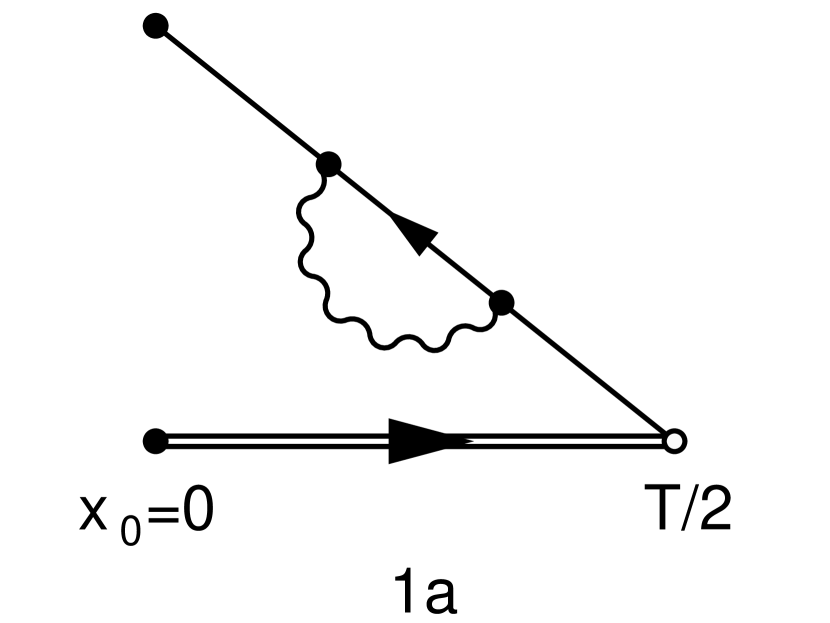
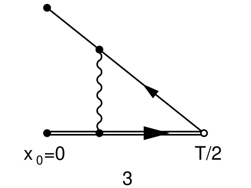
Figure 2: One loop diagrams contributing to $f_{\rm A}^{\rm stat}(T/2)$.

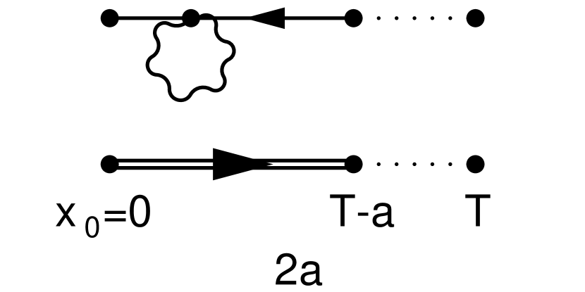
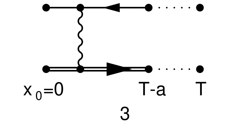
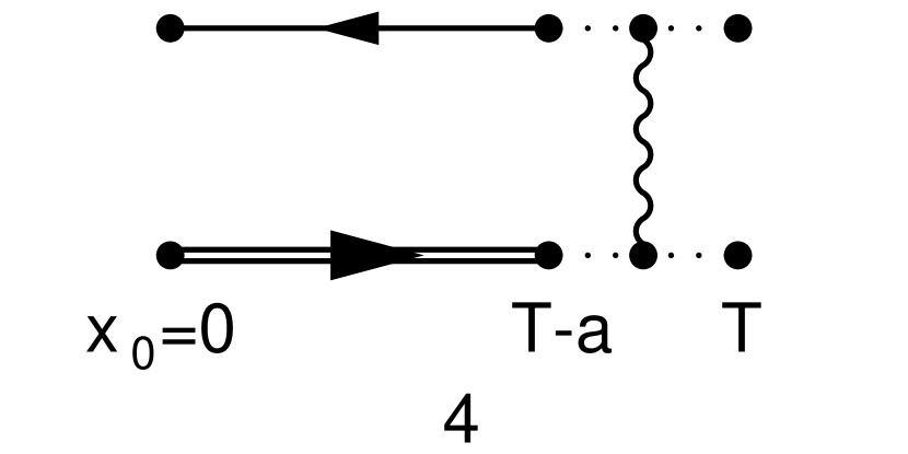
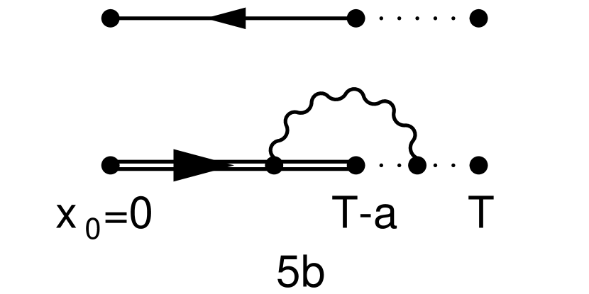
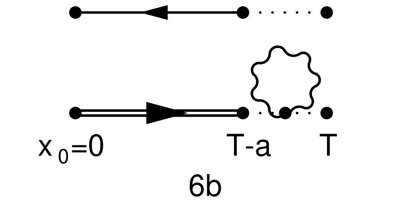
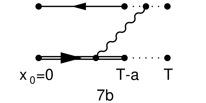
Figure 3: One loop diagrams contributing to $f_{1}^{\rm stat}$. The dotted lines denote the link from $T-a$ to T.

B.2 Calculation of $(c_{\rm A}^{\rm stat})^{(1)}$ and $(b_{\rm A}^{\rm stat})^{(1)}$

For the calculation of $(c_{\rm A}^{\rm stat})^{(1)}$, the one-loop coefficient of the ratio $X_{\rm I}$ is decomposed as

$$X_{\rm I}^{(1)}(L/a)=X^{(1)}(L/a)|_{\tilde{c}_{t}=1}+\tilde{c}_{t}^{(1)}aX_{\rm b}^{(0)}(L/a)+{c_{\rm A}^{\rm stat}}^{(1)}aX_{\delta\rm A}^{(0)}.$$ (B.15)

Defining the derivatives $\partial$ and $\partial^{\ast}$ by

$$\partial f(L/a) = {1\over a}\left\{f\left(\hbox{$L+a\over a$}\right)-f(L/a)\right\}$$ (B.16)

$$\partial^{\ast}f(L/a) = {1\over a}\left\{f(L/a)-f\left(\hbox{$L-a\over a$}\right)\right\},$$ (B.17)

the ${\rm O}(a)$ part of $X_{\rm lat}^{(1)}$ can be extracted to get

$${c_{\rm A}^{\rm stat}}^{(1)}={{\lim_{a/L\rightarrow 0}\hbox{$L^{2}\over 2a$}(\partial+\partial^{\ast})X_{\rm lat}^{(1)}(\hbox{$L\over a$})|_{\tilde{c}_{t}=1}-\lim_{a/L\rightarrow 0}\tilde{c}_{t}^{(1)}LX_{\rm b}^{(1)}(\hbox{$L\over a$})}\over{\lim_{a/L\rightarrow 0}LX_{\delta\rm A}^{(0)}(\hbox{$L\over a$})}}$$ (B.18)

with the light quark mass set to zero.

In a similar way, $(b_{\rm A}^{\rm stat})^{(1)}$ can be calculated,

$${b_{\rm A}^{\rm stat}}^{(1)} = \left\{\lim_{a/L\rightarrow 0}\hbox{$L^{2}\over 2a$}(\partial+\partial^{\ast})\tilde{X}^{(1)}(\hbox{$L\over a$})|_{\tilde{c}_{t}=1}-\lim_{a/L\rightarrow 0}\tilde{c}_{t}^{(1)}LX_{\rm b}^{(1)}(\hbox{$L\over a$})\right.$$ (B.19)

$$\left.\left.-\lim_{a/L\rightarrow 0}{c_{\rm A}^{\rm stat}}^{(1)}LX_{\delta\rm A}^{(0)}(\hbox{$L\over a$})\right\}\right/\left\{\lim_{a/L\rightarrow 0}zX^{(0)}(\hbox{$L\over a$})\right\},$$

where

$$\tilde{X}^{(1)}=(1+{b_{\rm A}^{\rm stat}}^{(0)}am_{\rm q}^{(0)})X^{(1)}+(Z_{\rm A,lat}^{\rm stat(1)}+{b_{\rm A}^{\rm stat}}^{(0)}am_{\rm q}^{(1)})X^{(0)}.$$ (B.20)

The quantity

$$z=Z_{\rm m,lat}(1+b_{\rm m}am_{\rm q})Lm_{\rm q}$$ (B.21)

is kept fixed when taking the limit. The renormalization and improvement constants for the light quark mass are known from [41].

Appendix C Numerical results

The following results were obtained at $T=L$, with the bare light quark mass set to the critical mass

$$m_{\rm c}=m_{\rm c}^{(1)}g_{0}^{2}+O(g_{0}^{4}),$$ (C.1)

with [8]

$$am_{\rm c}^{(1)}=-0.2025565\times C_{\rm F}.$$ (C.2)

The improvement coefficients used are

$$c_{\rm sw}=1,$$ (C.3)

and

$$\tilde{c}_{t}=1+\tilde{c}_{t}^{(1)}g_{0}^{2}+O(g_{0}^{4}),$$ (C.4)

with [41]

$$\tilde{c}_{t}^{(1)}=-0.01346\times C_{\rm F}.$$ (C.5)

The tree level results can be obtained analytically. Using the notation of [8], they are

$${f_{\rm A}^{\rm stat}}^{(0)}(x_{0}) = -{3\over{R(p^{+})}}\{(M(p^{+})-\stackrel{{\scriptstyle\circ}}{{p}}_{0}^{+})e^{-\omega({\it\bf p}^{+})x_{0}}$$ (C.6)

$$-((M(p^{+})+\stackrel{{\scriptstyle\circ}}{{p}}_{0}^{+})e^{-\omega({\it\bf p}^{+})(2L-x_{0})}\}\qquad{\rm at}\quad{\it\bf p}={\it\bf 0},$$

and

$${f_{1}^{\rm stat}}^{(0)} = {3\over{R(p^{+})}}\{(M(p^{+})-\stackrel{{\scriptstyle\circ}}{{p}}_{0}^{+})e^{-\omega({\it\bf p}^{+})(L-a)}$$ (C.7)

$$-((M(p^{+})+\stackrel{{\scriptstyle\circ}}{{p}}_{0}^{+})e^{-\omega({\it\bf p}^{+})(L+a)}\}\qquad{\rm at}\quad{\it\bf p}={\it\bf 0}.$$

Also the axial current improvement term can be calculated analytically at tree level,

$${f_{\delta\rm A}^{\rm stat}}^{(0)}(x_{0})=-{3(\stackrel{{\scriptstyle\circ}}{{{\it\bf p}}}^{+})^{2}\over{R(p^{+})}}\{e^{-\omega({\it\bf p}^{+})x_{0}}-e^{-\omega({\it\bf p}^{+})(2L-x_{0})}\}\qquad{\rm at}\quad{\it\bf p}={\it\bf 0}.$$ (C.8)

The one loop results are given tables (2)– (4). They have been obtained in double precision calculations. Where an error is given, it has been taken from the comparison with the corresponding quadruple precision result.

$L/a$	${f_{\rm A}^{\rm stat}}^{(1)}(L/2)$		${f_{1}^{\rm stat}}^{(1)}$
4	1.	1696384959451731(7)	$-2$.	788717306605536(2)
6	1.	5721721053841535	$-3$.	744847208299456
8	2.	049414037209983(4)	$-4$.	76922384055426(4)
10	2.	543921176114074	$-5$.	80311014058304
12	3.	04401042107373(4)	$-6$.	8365479914505(2)
14	3.	54641935327602	$-7$.	86798061045362
16	4.	04997105269991(6)	$-8$.	897379383110(2)
18	4.	55415464879211	$-9$.	924989104618
20	5.	058717578768(1)	$-10$.	951072803831(9)
22	5.	5635226305105	$-11$.	975859714707
24	6.	0684897524216	$-12$.	999539542806
26	6.	5735695645449	$-14$.	02226731358
28	7.	0787302119581	$-15$.	04416980198
30	7.	583950374904	$-16$.	06535128339
32	8.	089215337913	$-17$.	08589819107
34	8.	594514673902	$-18$.	10588276384
36	9.	099840825103	$-19$.	12536587521
38	9.	60518820413	$-20$.	14439922726
40	10.	11055260756	$-21$.	1630270594
42	10.	61593082380	$-22$.	1812874905
44	11.	12132036473	$-23$.	1992135777
46	11.	62671927843	$-24$.	2168341613
48	12.	1321260162(3)	$-25$.	234174544(1)

Table 2: $f_{\rm A}^{\rm stat}$ and $f_{1}^{\rm stat}$ at one loop order with $\theta=0.0$

$L/a$	${f_{\rm A}^{\rm stat}}^{(1)}(L/2)$	${f_{1}^{\rm stat}}^{(1)}$
4	0.707462157465912(1)	$-1$.	828520866963525(4)
6	1.0665692749675324	$-2$.	53494068630446456
8	1.45264489740883(2)	$-3$.	268670455891038(1)
10	1.845191095078847	$-4$.	0063158459818604
12	2.23966783029017(2)	$-4$.	7434246150126(1)
14	2.634843388684698	$-5$.	47929315793510
16	3.03031175469344(4)	$-6$.	2139336444356(4)
18	3.42591623855986	$-6$.	9474888408264
20	3.82158857585887	$-7$.	6801091376222
22	4.21729615057110	$-8$.	4119266083201
24	4.61302225619736	$-9$.	1430518919882
26	5.00875788592884	$-9$.	8735765450344
28	5.40449800734282	$-10$.	603576331834
30	5.80023974629234	$-11$.	333114250324
32	6.19598144778345	$-12$.	062243035152
34	6.59172216643778	$-12$.	791007154176
36	6.98746137900958	$-13$.	51944438137
38	7.3831988169726	$-14$.	24758703382
40	7.7789343665427	$-14$.	97546294777
42	8.1746680077261	$-15$.	70309625284
44	8.5703997766495	$-16$.	43050799027
46	8.9661297419670	$-17$.	1577166104
48	9.36185799001(1)	$-17$.	8847383757(5)

Table 3: $f_{\rm A}^{\rm stat}$ and $f_{1}^{\rm stat}$ at one loop order with $\theta=0.5$

$L/a$	${f_{\rm A}^{\rm stat}}^{(1)}(L/2)$	${f_{1}^{\rm stat}}^{(1)}$
4	0.3044333805556540(7)	$-0$.869671412347571(1)
6	0.5486322003500290	$-1$.1948835905593809
8	0.793695141003886(4)	$-1$.53524521245116(1)
10	1.038456376564977	$-1$.881017287644124
12	1.28269652915735(3)	$-2$.22894706469196(3)
14	1.52651219643810	$-2$.57783369422662
16	1.77002559881285(11)	$-2$.92715777151496(7)
18	2.01332870498098	$-3$.27666836444461
20	2.2564839354402(4)	$-3$.6262359702708(2)
22	2.4995329275626	$-3$.97579139115074
24	2.7425037517644	$-4$.3252973303331
26	2.9854157215170	$-4$.6747341210386
28	3.2282824349472	$-5$.0240921351849
30	3.4711136865628	$-5$.3733675663630
32	3.7139166829809	$-5$.7225600072263
34	3.9566968307148	$-6$.071671021232
36	4.199458257584	$-6$.420703284271
38	4.442204165276	$-6$.769660062007
40	4.684937072624	$-7$.118544889597
42	4.927658986791	$-7$.467361375608
44	5.170371525823	$-7$.81611308330
46	5.413076007854	$-8$.16480346057
48	5.65577351702(2)	$-8$.51343580067(7)

Table 4: $f_{\rm A}^{\rm stat}$ and $f_{1}^{\rm stat}$ at one loop order with $\theta=1.0$

References

• [1] BaBar Collab., D. Boutigni et al., SLAC-R-457 (1995), Technical Design Report.
• [2] BELLE Collab., M.T. Cheng et al., KEK-Report 95-1 (1995), Technical Design Report.
• [3] HERA-B Collab., E. Hartouni et al., DESY-PRC 95/01 (1995), Technical Design Report.
• [4] M. Lüscher, (1997), hep-ph/9711205.
• [5] H. Wittig, (1999), hep-ph/9911400.
• [6] ALPHA and UKQCD, J. Garden, J. Heitger, R. Sommer and H. Wittig, (1999), hep-lat/9906013.
• [7] M. Lüscher, S. Sint, R. Sommer and P. Weisz, Nucl. Phys. B478 (1996) 365, hep-lat/9605038.
• [8] M. Lüscher and P. Weisz, Nucl. Phys. B479 (1996) 429, hep-lat/9606016.
• [9] M. Lüscher, S. Sint, R. Sommer, P. Weisz and U. Wolff, Nucl. Phys. B491 (1997) 323, hep-lat/9609035.
• [10] M. Lüscher, S. Sint, R. Sommer and H. Wittig, Nucl. Phys. B491 (1997) 344, hep-lat/9611015.
• [11] R. Sommer, Phys. Rept. 275 (1996) 1, hep-lat/9401037.
• [12] H. Wittig, Int. J. Mod. Phys. A12 (1997) 4477, hep-lat/9705034.
• [13] S. Hashimoto, (1999), hep-lat/9909136.
• [14] E. Eichten and B. Hill, Phys. Lett. B234 (1990) 511.
• [15] M. Neubert, Phys. Rept. 245 (1994) 259, hep-ph/9306320, and references therein.
• [16] N. Isgur and M.B. Wise, Phys. Lett. B232 (1989) 113.
• [17] N. Isgur and M.B. Wise, Phys. Lett. B237 (1990) 527.
• [18] H. Georgi, Phys. Lett. B240 (1990) 447.
• [19] C. Alexandrou et al., Z. Phys. C62 (1994) 659, hep-lat/9312051.
• [20] ALPHA, M. Guagnelli, J. Heitger, R. Sommer and H. Wittig, Nucl. Phys. B560 (1999) 465, hep-lat/9903040.
• [21] UKQCD, C. Michael and J. Peisa, (1998), hep-lat/9802015.
• [22] A. Duncan, E. Eichten and H. Thacker, Phys. Lett. B303 (1993) 109.
• [23] M. Kurth and R. Sommer, Nucl. Phys. Proc. Suppl. 83-84 (2000) 857, hep-lat/9908039.
• [24] A. Donini et al., Nucl. Phys. Proc. Suppl. 47 (1996) 489, hep-lat/9509078.
• [25] C.T. Sachrajda, private communications.
• [26] J. Heitger, M. Kurth and R. Sommer, in preparation.
• [27] B. Sheikholeslami and R. Wohlert, Nucl. Phys. B259 (1985) 572.
• [28] P. Boucaud, C.L. Lin and O. Pène, Phys. Rev. D40 (1989) 1529, Erratum Phys. Rev. D41 (1990) 3541.
• [29] E. Eichten and B. Hill, Phys. Lett. B240 (1990) 193.
• [30] P. Boucaud, J.P. Leroy, J. Micheli, O. Pène and G.C. Rossi, Phys. Rev. D47 (1993) 1206.
• [31] L. Maiani, G. Martinelli and C.T. Sachrajda, Nucl. Phys. B368 (1992) 281.
• [32] T. Reisz, Nucl. Phys. B318 (1989) 417.
• [33] A. Borrelli and C. Pittori, Nucl. Phys. B385 (1992) 502.
• [34] G. Martinelli and C.T. Sachrajda, Nucl. Phys. B559 (1999) 429, hep-lat/9812001.
• [35] K. Symanzik, Nucl. Phys. B226 (1983) 205.
• [36] M. Lüscher and P. Weisz, Commun. Math. Phys. 97 (1985) 59.
• [37] C. Morningstar and J. Shigemitsu, Phys. Rev. D57 (1998), hep-lat/9712015.
• [38] M. Lüscher, R. Narayanan, P. Weisz and U. Wolff, Nucl. Phys. B384 (1992) 168, hep-lat/9207009.
• [39] S. Sint, Nucl. Phys. B421 (1994) 135, hep-lat/9312079.
• [40] S. Sint, Nucl. Phys. B451 (1995) 416, hep-lat/9504005.
• [41] S. Sint and P. Weisz, Nucl. Phys. B502 (1997) 251, hep-lat/9704001.
• [42] M.A. Shifman and M.B. Voloshin, Sov. J. Nucl. Phys. 45 (1987) 292.
• [43] H.D. Politzer and M.B. Wise, Phys. Lett. B206 (1988) 681.
• [44] ALPHA, A. Bode, P. Weisz and U. Wolff, Nucl. Phys. B576 (2000) 517, hep-lat/9911018.
• [45] X. Ji and M.J. Musolf, Phys. Lett. B257 (1991) 409.
• [46] M. Kurth and R. Sommer, in preparation.
• [47] M. Lüscher, R. Sommer, P. Weisz and U. Wolff, Nucl. Phys. B413 (1994) 481, hep-lat/9309005.
• [48] D.J. Broadhurst and A.G. Grozin, Phys. Lett. B267 (1991) 105.
• [49] V. Gimenez, Nucl. Phys. B375 (1992) 582.
• [50] S. Sint and R. Sommer, Nucl. Phys. B465 (1996) 71, hep-lat/9508012.
• [51] ALPHA, S. Sint and P. Weisz, Nucl. Phys. B545 (1999) 529, hep-lat/9808013.
• [52] ALPHA, S. Capitani, M. Lüscher, R. Sommer and H. Wittig, Nucl. Phys. B544 (1999) 669, hep-lat/9810063.
• [53] K.I. Ishikawa, T. Onogi and N. Yamada, Nucl. Phys. Proc. Suppl. 83 (2000) 301, hep-lat/9909159.