UTCCP-P-88

June 2000

On the Determination of Nonleptonic Kaon Decays

from $K\to\pi$ Matrix Elements

Maarten Golterman¹

Center for Computational Physics, University of Tsukuba, Tsukuba,

Ibaraki 305-8577, Japan

and

Department of Physics, Washington University, St. Louis, MO 63130, USA^∗

Elisabetta Pallante²

Facultat de Física, Universitat de Barcelona, Diagonal 647, 08028 Barcelona, Spain

Abstract

The coupling constants of the order $p^{2}$ low-energy weak effective lagrangian can be determined from the $K\to\pi$ and $K\to 0$ weak matrix elements, choosing degenerate quark masses for the first of these. However, for typical values of quark masses in Lattice QCD computations, next-to-leading $O(p^{4})$ corrections are too large to be ignored, and will need to be included in future analyses. Here we provide the complete $O(p^{4})$ expressions for these matrix elements obtained from Chiral Perturbation Theory, valid for partially quenched QCD with $N$ degenerate sea quarks. Quenched QCD corresponds to the special case $N=0$. We also discuss the role of the $\eta^{\prime}$ meson in some detail, and we give numerical examples of the size of chiral logarithms.

PACS: 13.25.Es, 12.38.Gc, 12.39.Fe

^∗ permanent address
¹ e-mail: maarten@aapje.wustl.edu
² e-mail: pallante@ecm.ub.es

1 Introduction

The determination of non-leptonic kaon-decay amplitudes from Lattice QCD remains a challenging task. However, recently there have been several developments which may lead to substantial progress in this field, ranging from new ideas on how to cope with chiral symmetry on the lattice to a sizable increase of computer power available for the necessary numerical computations.

Still, there are important theoretical difficulties afflicting the determination of the relevant weak matrix elements, which are a consequence of the fact that the final states contain more than one strongly interacting particle (the pions). This is formalized in what is sometimes called the Maiani–Testa theorem [1], which says that it is not possible to extract the physical matrix elements with the correct kinematics from the asymptotic behavior in time of the euclidean correlation functions accessible to numerical computation.

There are several old and new ideas on the market on how to deal with this situation, which divide into three groups. First, one may determine the matrix elements with a kaon in the initial state and two (or more) pions in the final state for an unphysical choice of external momenta. From the large-time behavior of the euclidean correlation function

$$C(t_{2},t_{1})=\langle 0|\pi_{1}(t_{2})\pi_{2}(t_{2}){\cal O}_{\rm weak}(t_{1})K(0)|0\rangle\;,$$ (1.1)

with the kaon at rest, one obtains the matrix element for ${\vec{p}}\equiv{\vec{p}}_{\pi_{1}}=-{\vec{p}}_{\pi_{2}}=0$ instead of the physical $|{\vec{p}}|=(1/2)\sqrt{m_{K}^{2}-4m_{\pi}^{2}}$, i.e. energy is not conserved [1, 2]. The idea is then to use chiral perturbation theory (ChPT) in order to correct for this unphysical choice of momenta [3]. The most recent computation of the $\Delta I=3/2$ $K\to 2\pi$ matrix element using this method can be found in Ref. [4]. In this computation, all meson masses were taken degenerate and the quenched approximation was used. Adjustments for all these unphysical effects, which also include power-like finite-volume effects coming from pion rescattering diagrams, were made using one-loop ChPT [2]. For recent ideas on choosing $m_{K}=2m_{\pi}$ for the lattice computation (for which ${\vec{p}}=0$ does conserve energy), see Refs. [5, 6].

For the $\Delta I=1/2$ case, the situation is more complicated for a number of reasons. Here we only mention (since this is less well known) that a quenched or partially quenched computation appears to be afflicted by “enhanced finite-volume effects,” which do not occur for the $\Delta I=3/2$ case. This problem appears at one–loop in quenched ChPT [7, 8], but not much is known about this effect beyond one loop. We are investigating this issue. For a nice review of many other issues, see Ref. [5].

A second idea was very recently proposed in Ref. [9], where it was shown how the matrix elements of interest can in principle be determined from finite-volume correlation functions without analytic continuation. The energy-conserving amplitude is obtained by tuning the spatial volume such that the first excited level of the two-pion final state has an energy equal to the kaon mass. With sufficient accuracy to determine the lowest excited levels, the finite-volume matrix element may then be computed on the lattice, and subsequently be converted into the physical infinite-volume amplitude. For this, it is obviously necessary to choose meson masses such that $2m_{\pi}<m_{K}$ (as well as $m_{K}<4m_{\pi}$, so that the final-state pions are in the elastic regime). Again, if such a computation is done in a (partially) quenched setting one might expect that enhanced finite-volume effects could also occur with this method.

A third idea is based on the observation that, if one needs ChPT anyway in order to convert an unphysical matrix element into a physical one, one might as well choose the unphysical matrix element as simple as possible. Chiral symmetry relates the $K\to 2\pi$ matrix elements of interest to the simpler $K\to\pi$ and $K\to$ vacuum ($K\to 0$) matrix elements of the same weak operators which mediate non-leptonic kaon decay [10]. Advantages of this approach are that there are no strongly interacting particles in the final state, and that lattice computations of these simpler matrix elements may be less difficult.

The first advantage is, in a sense, not really an advantage if one wishes to convert the results of a lattice computation into a calculation of the non-leptonic kaon decay rates, because final-state interactions will still have to be taken into account. However, this method does avoid all the unphysical effects, such as power-like or even enhanced finite-volume effects, associated with the multi-pion final state. Formulated in another way, with this method the simplest possible matrix elements (in this case $K\to\pi$ and $K\to 0$) are used to obtain the relevant weak low-energy constants (LECs) of the weak effective lagrangian. Using ChPT, these can then be converted into estimates of the kaon-decay rates.

A key question is which order in ChPT will be needed in order to carry out such a program. At tree level (i.e. $O(p^{2})$), only three LECs come into play, but at one loop (i.e. $O(p^{4})$) many more LECs contribute to all relevant matrix elements [11]. In fact, from the analysis reported in this paper as well as from previous work it is clear that tree-level ChPT is not enough [2, 7, 12]. In addition (as we will demonstrate), not all $O(p^{4})$ LECs needed for $K\to 2\pi$ decays can be obtained from $K\to\pi$ and $K\to 0$ matrix elements. However, as we will advocate in this paper, it may be possible to determine at least the $O(p^{2})$ LECs from a lattice computation, taking one-loop ChPT effects into account. A reliable, first-principle determination of the $O(p^{2})$ octet and 27-plet LECs would clearly be interesting by itself. Moreover, phenomenological estimates of these LECs, based on a one-loop ChPT analysis of experimental data are available [13], making a direct comparison possible.

In this paper we present an analysis of $K\to\pi$ and $K\to 0$ amplitudes in one-loop ChPT, with the above described philosophy in mind. For $K\to\pi$ we choose our valence quark masses to be degenerate, thus conserving energy for this case. The analysis is performed in partially quenched ChPT [14], with an arbitrary number of degenerate sea quarks. We present the results for these matrix elements in terms of the quark masses.

In Sect. 2, we list and discuss all $O(p^{2})$ and $O(p^{4})$ operators needed for our calculation, including those containing the $\eta^{\prime}$ meson. In Sect. 3, we discuss the role of the $\eta^{\prime}$ in partially quenched QCD in some more detail than has been done so far in the literature. This section can be skipped if one is only interested in results. In Sect. 4, we give complete one-loop expressions for the octet and 27-plet $K\to\pi$ and $K\to 0$ matrix elements, including contributions from $O(p^{4})$ operators, organized by subsection. In Subsect. 4.1 partially quenched results for $N$ degenerate sea quarks are presented, which are valid also in the case that the meson made out of sea quarks (the “sea meson”) is not light compared to the $\eta^{\prime}$ (a realistic situation in actual lattice computations). In Subsect. 4.2 we specialize to the case that the sea meson is light compared to the $\eta^{\prime}$. Subsect. 4.3 contains the completely quenched results, obtained by setting $N=0$ and keeping the $\eta^{\prime}$. For completeness, we include the fully unquenched results, with non-degenerate sea-quark masses for the $K\to 0$ matrix elements, in Subsect. 4.4. In Sect. 5 we present a detailed discussion of the results, including the role of $O(p^{4})$ operators and numerical examples for typical choices of the parameters. The last section contains our conclusions.

2 Definition of operators

Partially quenched QCD may be defined by separately introducing valence- and sea-quark fields, each with their own mass. The valence quarks are quenched by introducing for each valence quark a “ghost” quark, which has the same mass and quantum numbers, but opposite statistics [14, 15]. This, in effect, removes the valence-quark determinant from the QCD partition function. We will consider a theory with $n$ quarks, of which $N$ are sea quarks, and $n-N\geq 3$ valence quarks. This requires $n-N$ ghost quarks, with masses equal to those of the valence quarks. We will consider valence quarks with arbitrary masses $m_{1},\dots,m_{n-N}$, and degenerate sea quarks, all with mass $m_{S}$. The relevant chiral symmetry group is the graded group SU($n|n-N$)${}_{L}\otimes$SU($n|n-N$)_R [14]. Fully quenched QCD arises as a special case of this construction by taking $N=0$ [16], or equivalently, when the sea quarks are decoupled by taking $m_{S}\to\infty$.

The euclidean low-energy effective lagrangian which mediates non-leptonic weak transitions with $\Delta S=1$ is given by

$${\cal L}_{\Delta S=1}={\cal L}_{2}+{\cal L}_{2}^{\eta^{\prime}}+{\cal L}_{4}+\ldots\;,$$ (2.1)

where the dots denote higher order terms in the chiral expansion. The $O(p^{2})$ lagrangian [10] ${\cal L}_{2}$ contains three terms

$${\cal L}_{2}=-\alpha^{8}_{1}\,{\mbox{str}\,}(\Lambda L_{\mu}L_{\mu})+\alpha^{8}_{2}\,{\mbox{str}\,}(\Lambda X_{+})+\alpha^{27}\,T^{ij}_{kl}(L_{\mu})^{k}_{\ i}(L_{\mu})^{l}_{\ j}+{\mbox{h.c.}}\;,$$ (2.2)

where str  denotes the supertrace in flavor space. Note that the supertraces become normal traces, ${\mbox{str}\,}\to{\mbox{tr}\,}$, in the case $N=n$. The terms with couplings $\alpha^{8}_{1},\alpha^{8}_{2}$ transform as $(8_{L},1_{R})$, while the term with coupling $\alpha^{27}$ transforms as $(27_{L},1_{R})$. The order $p^{2}$ lagrangian ${\cal L}_{2}^{\eta^{\prime}}$ will be discussed toward the end of this section. The $O(p^{4})$ lagrangian can be written as

$${\cal L}_{4}=\frac{1}{(4\pi f)^{2}}\left(\sum_{i}\beta^{8}_{i}\,{\cal O}^{8}_{i}+\sum_{i}{\tilde{\beta}}^{8}_{i}\,{\tilde{\cal O}}^{8}_{i}+\sum_{i}\beta^{27}_{i}\,{\cal O}^{27}_{i}\right)\;,$$ (2.3)

with $(8_{L},1_{R})$ $O(p^{4})$ operators ${\cal O}^{8}_{i}$, ${\tilde{\cal O}}^{8}_{i}$ and $(27_{L},1_{R})$ $O(p^{4})$ operators ${\cal O}^{27}_{i}$ [11, 12, 17]. The operators ${\tilde{\cal O}}^{8}_{i}$ denote total-derivative operators; they do not contribute to energy-momentum conserving matrix elements. However, they do contribute to the $K\to 0$ matrix element, which does not conserve energy for non-degenerate quark masses. Note that there are no 27-plet total-derivative operators that contribute to the matrix elements considered in this paper, to $O(p^{4})$. The fields entering the weak operators are defined as follows

$$L_{\mu} = i\Sigma\partial_{\mu}\Sigma^{\dagger}\;,$$ (2.4)

$$X_{\pm} = 2B_{0}(\Sigma M^{\dagger}\pm M\Sigma^{\dagger})\;,$$

where $B_{0}$ is the parameter $B_{0}$ of Ref. [18] and $B_{0}=4v/f^{2}$ in the notation of Ref. [10]. The unitary field $\Sigma$ is defined in terms of the hermitian field $\Phi$ describing the Goldstone meson multiplet as

$$\Sigma={\mbox{exp}\,}(2i\Phi/f)\;,$$ (2.5)

where $f$ is the bare pion-decay constant, normalized such that $f_{\pi}=132$ MeV. Note that $L_{\mu}$ and $X_{\pm}$ transform as $(8_{L},1_{R})$ under (valence-flavor) SU(3)${}_{L}\otimes$SU(3)_R. The matrix $\Lambda$ in the lagrangian (2.2) picks out the $\Delta S=1$, $\Delta D=-1$ part of the octet operators, all with $\Delta I=1/2$:

$$\Lambda^{i}_{\ j}=\delta^{i3}\delta_{j2}\;,$$ (2.6)

where $i,j=1,2,3\ldots$ (or $u,d,s\ldots$) denote valence flavors. The tensor $T^{ij}_{kl}$ projects onto the $\Delta I=1/2$ part of the $(27_{L},1_{R})$ operator, with nonzero components

$$T^{13}_{12} = T^{31}_{12}=T^{13}_{21}=T^{31}_{21}=\frac{1}{2}\;,$$ (2.7)

$$T^{23}_{22} = T^{32}_{22}=1\;,$$

$$T^{33}_{32} = T^{33}_{23}=-\frac{3}{2}\;,$$

or onto the $\Delta I=3/2$ part, with nonzero components

$$T^{13}_{12} = T^{31}_{12}=T^{13}_{21}=T^{31}_{21}=\frac{1}{2}\;,$$ (2.8)

$$T^{23}_{22} = T^{32}_{22}=-\frac{1}{2}\;.$$

The term with coupling $\alpha^{8}_{2}$ is known as the “weak mass term,” and mediates the $K\to 0$ transition at tree level. Its odd-parity part, which in principle can also contribute to the octet $K\to\pi\pi$ amplitude, is proportional to $m_{s}-m_{d}$. For $m_{s}\neq m_{d}$ the weak mass term is a total derivative [10, 19], and therefore does not contribute to any energy-momentum-conserving physical matrix element, like $K\to\pi\pi$. Instead, the $K\to 0$ and, for $M_{K}\neq M_{\pi}$, $K\to\pi$ matrix elements do not conserve energy, and therefore the weak mass term does contribute to both of them. For $m_{s}=m_{d}$ the weak mass term is not a total derivative, so that it contributes also to the $K\to\pi$ matrix element with $M_{K}=M_{\pi}$. Hence, in order to determine the octet coupling $\alpha^{8}_{1}$ from a computation of the $K\to\pi$ matrix element, another quantity such as the $K\to 0$ matrix element is always needed, in order to eliminate the dependence on $\alpha^{8}_{2}$.

At order $p^{4}$ there are eight $(8_{L},1_{R})$ operators and six $(27_{L},1_{R})$ operators which can contribute to $K\to 0$, $K\to\pi$ and $K\to\pi\pi$ matrix elements. The octet operators can be written as follows

$${\cal O}^{8}_{1} = {\mbox{str}\,}(\Lambda X_{+}X_{+})\;,$$ (2.9)

$${\cal O}^{8}_{2} = {\mbox{str}\,}(\Lambda X_{+})\,{\mbox{str}\,}(X_{+})\;,$$

$${\cal O}^{8}_{3} = {\mbox{str}\,}(\Lambda X_{-}X_{-})\;,$$

$${\cal O}^{8}_{5} = {\mbox{str}\,}(\Lambda[X_{+},X_{-}])\;,$$

$${\cal O}^{8}_{10} = {\mbox{str}\,}(\Lambda\{X_{+},L_{\mu}L_{\mu}\})\;,$$

$${\cal O}^{8}_{11} = {\mbox{str}\,}(\Lambda L_{\mu}X_{+}L_{\mu})\;,$$

$${\cal O}^{8}_{13} = {\mbox{str}\,}(\Lambda X_{+})\,{\mbox{str}\,}(L_{\mu}L_{\mu})\;,$$

$${\cal O}^{8}_{15} = {\mbox{str}\,}(\Lambda[X_{-},L_{\mu}L_{\mu}])\;,$$

while the 27-plet operators are

$${\cal O}^{27}_{1} = T^{ij}_{kl}(X_{+})^{k}_{\ i}(X_{+})^{l}_{\ j}\;,$$ (2.10)

$${\cal O}^{27}_{2} = T^{ij}_{kl}(X_{-})^{k}_{\ i}(X_{-})^{l}_{\ j}\;,$$

$${\cal O}^{27}_{4} = T^{ij}_{kl}(L_{\mu})^{k}_{\ i}(\{L_{\mu},X_{+}\})^{l}_{\ j}\;,$$

$${\cal O}^{27}_{5} = T^{ij}_{kl}(L_{\mu})^{k}_{\ i}([L_{\mu},X_{-}])^{l}_{\ j}\;,$$

$${\cal O}^{27}_{6} = T^{ij}_{kl}(X_{+})^{k}_{\ i}(L_{\mu}L_{\mu})^{l}_{\ j}\;,$$

$${\cal O}^{27}_{7} = T^{ij}_{kl}(L_{\mu})^{k}_{\ i}(L_{\mu})^{l}_{\ j}\,{\mbox{str}\,}(X_{+})\;.$$

These operators are the same as those in Ref. [19], apart from the replacement ${\mbox{tr}\,}\to{\mbox{str}\,}$. For the energy-momentum non-conserving matrix elements the only total-derivative term that is needed is

$${\tilde{\cal O}}^{8}_{1}=i\partial_{\mu}\,{\mbox{str}\,}(\Lambda[L_{\mu},X_{+}])\;.$$ (2.11)

In general, in the (partially) quenched formulation of the effective theory one needs to keep the $\eta^{\prime}$ [16, 20, 21, 22], defined as the SU($n|n-N$)${}_{L}\otimes$SU($n|n-N$)_R invariant [14]

$$\eta^{\prime}={\mbox{str}\,}(\Phi)\;.$$ (2.12)

Note that this normalization differs from the one in Ref. [14], but is more convenient in keeping track of $N$ dependence. The presence of the $\eta^{\prime}$ leads to new operators in the strong [16, 18] and weak effective lagrangians. Under CPS symmetry [10] all operators in ${\cal L}_{2,4}$ of Eq. (2.1) are even, and, since $\eta^{\prime}$ is CPS odd, new weak operators can be constructed by multiplying ${\cal L}_{2,4}$ by even powers of $\eta^{\prime}$. It turns out that such operators do not contribute to the quantities of interest in this paper. However, other new weak operators arise from multiplying CPS-odd weak operators by odd powers of $\eta^{\prime}$. There are two operators of interest at order $p^{2}$, so that ${\cal L}_{2}^{\eta^{\prime}}$ is given by

$${\cal L}_{2}^{\eta^{\prime}}=\gamma^{8}_{1}\,\partial_{\mu}(\eta^{\prime}/f){\mbox{str}\,}(\Lambda L_{\mu})+i\gamma^{8}_{2}\,(\eta^{\prime}/f){\mbox{str}\,}(\Lambda X_{-})\;.$$ (2.13)

Since we are not interested in processes with external $\eta^{\prime}$ lines, we do not consider new operators of order $p^{4}$ containing the $\eta^{\prime}$ field.

For $N=3$ sea quarks the dynamics of the partially quenched theory is precisely that of unquenched QCD with degenerate quark masses [14]. Since all the low-energy constants (LECs) $\alpha^{8}_{i},\,\alpha^{27}$, $\gamma^{8}_{i}$ and $\beta^{8,27}_{i},\,\tilde{\beta}_{i}^{8}$ (together with the strong counterterms) are independent of quark masses, it follows that their $N=3$ partially-quenched values are equal to those of the real world [23]. However, for this equivalence to be valid, the $\eta^{\prime}$ should be treated in the same way in the partially quenched theory as in the real world, so that one has to consider the limit in which the $\eta^{\prime}$ decouples.

3 The role of the $\eta^{\prime}$ in partially quenched ChPT

Before we present our results, we would like to discuss the role of the $\eta^{\prime}$ in a partially quenched theory in more detail. First, define the bare (or tree-level) meson masses

$$M^{2}_{ij}=B_{0}(m_{i}+m_{j})\;,~{}~{}~{}~{}~{}~{}~{}i,j=1,\ldots 2n-N\;,$$ (3.1)

for a light pseudoscalar (pseudo-Goldstone) meson made out of quarks or ghost quarks $i$ and $j$. For degenerate sea quarks, this simplifies to $M^{2}_{SS}=2B_{0}m_{S}$. The two-point function for neutral mesons $\Phi_{ii}$ (in that basis) is given by [14]

$$\langle\Phi_{ii}(x)\Phi_{jj}(0)\rangle = \int\frac{d^{4}p}{(2\pi)^{4}}\,e^{ipx}\,G_{i,j}(p)\;,$$

$$G_{i,j}(p) = \frac{\delta_{ij}\epsilon_{i}}{p^{2}+M^{2}_{ii}}-X_{ij}(p)\;,$$ (3.2)

$$X_{ij}(p) = \frac{1}{3+N\alpha}\;\frac{(m_{0}^{2}+\alpha p^{2})(p^{2}+M^{2}_{SS})}{(p^{2}+M^{2}_{ii})(p^{2}+M^{2}_{jj})(p^{2}+M^{2}_{\eta^{\prime}})}\;,$$

where

$$\epsilon_{i}=\cases{+1,&for $1\leq i\leq n$\cr-1,&for $n+1\leq i\leq 2n-N$\cr}$$

and the $\eta^{\prime}$ mass is given by

$$M^{2}_{\eta^{\prime}}=\frac{M^{2}_{SS}+Nm_{0}^{2}/3}{1+N\alpha/3}\;.$$ (3.3)

The parameters $m_{0}^{2}$ and $\alpha$ (not to be confused with $\alpha^{8,27}_{i}$) come from the strong-lagrangian $O(p^{2})$ operators quadratic in the $\eta^{\prime}$ field, $(Nm_{0}^{2}/6)(\eta^{\prime})^{2}+(N\alpha/6)(\partial_{\mu}\eta^{\prime})^{2}$. The term $X_{ij}(p)$ has a double pole for $M_{ii}=M_{jj}$, unless $M_{SS}=M_{ii}=M_{jj}$. This implies that partially quenched theories suffer from the same “quenched infrared diseases” as the quenched theory unless all valence-quark masses are equal to the sea-quark mass [14]. From Eq. (3.2) it is easily verified that the $\eta^{\prime}$ two-point function is just $(N/(1+N\alpha/3))(p^{2}+M^{2}_{\eta^{\prime}})^{-1}$.

The quantity $X_{ij}(p)$ can also be written as

$$X_{ij}(p) = \frac{1}{3}\left(\frac{A_{ij}}{p^{2}+M^{2}_{ii}}\,-\,\frac{B_{ij}}{p^{2}+M_{\eta^{\prime}}^{2}}+\frac{{\cal M}^{2}_{ij}-A_{ij}M^{2}_{jj}}{(p^{2}+M^{2}_{ii})(p^{2}+M^{2}_{jj})}\right)\;,$$ (3.4)

with

$${\cal M}^{2}_{ij} = \frac{(N/3)(m_{0}^{2}-\alpha M_{ii}^{2})(m_{0}^{2}-\alpha M_{jj}^{2})M_{SS}^{2}+m_{0}^{2}(M_{SS}^{2}-M_{ii}^{2})(M_{SS}^{2}-M_{jj}^{2})}{[(N/3)(m_{0}^{2}-\alpha M_{ii}^{2})+M_{SS}^{2}-M_{ii}^{2}][(N/3)(m_{0}^{2}-\alpha M_{jj}^{2})+M_{SS}^{2}-M_{jj}^{2}]}\;,$$

$$A_{ij} = \frac{(N/3)(m_{0}^{2}-\alpha M_{ii}^{2})(m_{0}^{2}-\alpha M_{jj}^{2})+\alpha(M_{SS}^{2}-M_{ii}^{2})(M_{SS}^{2}-M_{jj}^{2})}{[(N/3)(m_{0}^{2}-\alpha M_{ii}^{2})+M_{SS}^{2}-M_{ii}^{2}][(N/3)(m_{0}^{2}-\alpha M_{jj}^{2})+M_{SS}^{2}-M_{jj}^{2}]}\;,$$

$$B_{ij} = \frac{(N/3)(m_{0}^{2}-\alpha M_{SS}^{2})^{2}/(1+\alpha N/3)}{[(N/3)(m_{0}^{2}-\alpha M_{ii}^{2})+M_{SS}^{2}-M_{ii}^{2}][(N/3)(m_{0}^{2}-\alpha M_{jj}^{2})+M_{SS}^{2}-M_{jj}^{2}]}\;.$$

The coefficients $A_{ij}$, $B_{ij}$ and ${\cal M}^{2}_{ij}$ are complicated functions of the various mass scales in the partially quenched effective theory. We may consider various limits in which these expressions simplify considerably. First, one easily obtains the fully quenched expression by setting $N=0$, or equivalently taking $M_{SS}\to\infty$, finding for all $ij$

$${\cal M}^{2}_{ij}\to m_{0}^{2}\;,\ \ \ A_{ij}\to\alpha\;,\ \ \ B_{ij}\to 0\;.$$ (3.6)

It is clear from these expressions that in the quenched case, the $\eta^{\prime}$ should be kept in the effective theory. Another interesting limit is that in which the $\eta^{\prime}$ decouples [23] (which, as inspection of Eq. (3.3) tells us, is only possible for $N>0$). In this limit, again for all $ij$,

$${\cal M}^{2}_{ij}\to\frac{3}{N}M_{SS}^{2}\;,\ \ \ A_{ij}\to\frac{3}{N}\;,$$ (3.7)

and we drop the $\eta^{\prime}$ pole in Eq. (3.4). The dependence of $X_{ij}$ on the $\eta^{\prime}$ parameters has disappeared in this limit.

As argued in Ref. [20], in actual partially quenched Lattice QCD computations, the sea-meson mass $M_{SS}$ maybe comparable in size to $m_{0}$ so that the full dependence of ${\cal M}^{2}_{ij}$ and $A_{ij}$ on the parameters $m_{0}$, $\alpha$ and $M_{SS}$ should be kept. A third possibility is then given by the limit in which the valence-meson mass is small compared to the $\eta^{\prime}$ mass, i.e. $M_{kk}\ll M_{\eta^{\prime}}$. The expressions for ${\cal M}^{2}_{ij}$, $A_{ij}$ and $B_{ij}$ given in Eq. (LABEL:MAB) reduce to those of Ref. [20] if we expand in $M_{kk}^{2}/M_{\eta^{\prime}}^{2}$ but not in $M_{SS}^{2}/M_{\eta^{\prime}}^{2}$:

$${\cal M}^{2}_{ij} \to {\cal M}^{2}=\frac{m_{0}^{2}M_{SS}^{2}}{(N/3)m_{0}^{2}+M_{SS}^{2}}\left(1+O\left(\frac{M_{kk}^{4}}{M_{\eta^{\prime}}^{4}}\right)\right)\;,$$ (3.8)

$$A_{ij} \to A=\frac{(N/3)m_{0}^{4}+\alpha M_{SS}^{4}}{[(N/3)m_{0}^{2}+M_{SS}^{2}]^{2}}+O\left(\frac{M_{kk}^{2}}{M_{\eta^{\prime}}^{2}}\right)\;,$$

$$B_{ij} \to \frac{(N/3)(m_{0}^{2}-\alpha M_{SS}^{2})^{2}/(1+\alpha N/3)}{[(N/3)m_{0}^{2}+M_{SS}^{2}]^{2}}+O\left(\frac{M_{kk}^{2}}{M_{\eta^{\prime}}^{2}}\right)\;.$$

The (partially) quenched expansion we consider in this paper is systematic if we take ${\cal M}^{2}$ to be of order $p^{2}$, in other words, if we take the parameter $m_{0}^{2}$ to be of the same order as the quark mass, just as in the case of quenched ChPT [16, 20, 24].

It was also shown in Ref. [20] that, for the quantities considered there, simply ignoring one-loop contributions coming from the $\eta^{\prime}$ pole in Eq. (3.4) and then taking the limit $M_{\eta^{\prime}}\to\infty$ in the rest is the same as matching to the limit in which the $\eta^{\prime}$ decouples. In other words, if we ignore these contributions, the LECs appearing in those quantities are the same in the $N=3$ partially quenched world and the real world. In addition, when we take only $M_{\eta^{\prime}}/M_{kk}$ large, but not $M_{\eta^{\prime}}/M_{SS}$, these one-loop contributions are polynomial in the valence-meson masses, and can still be ignored if we are interested in the non-analytic dependence on the valence-meson masses.

The same observations are also true here, even though there are diagrams with a more complicated topology than the simple tadpole diagrams needed in Ref. [20]. For $K\to\pi$, there are contributions of the form depicted in Fig. 1.

Figure 1: A diagram contributing to the $\Delta S=1$ $K\to\pi$ matrix element. A line is a pseudoscalar meson propagator, a dot a strong vertex and a box is a weak vertex.

Taking $M=M_{kk}$ to be the degenerate valence-meson mass running in the loop and abbreviating $B=B_{kk}$, this diagram leads to one-loop integrals such as

$$\int\frac{d^{4}p}{(2\pi)^{4}}\;\frac{1}{p^{2}+M^{2}}\;\frac{B}{p^{2}+M^{2}_{\eta^{\prime}}}=\frac{B}{M_{\eta^{\prime}}^{2}-M^{2}}\int\frac{d^{4}p}{(2\pi)^{4}}\left(\frac{1}{p^{2}+M^{2}}-\frac{1}{p^{2}+M^{2}_{\eta^{\prime}}}\right)\;,$$ (3.9)

multiplied by two powers of $M^{2}$ from the two $O(p^{2})$ vertices in the diagram (there are no contributions from vertices proportional to $M_{SS}^{2}$, so the only dependence on $M_{SS}$ comes through the coefficient $B$). The integral contributes an $\eta^{\prime}$ chiral logarithm, which we drop as above, and a Goldstone chiral logarithm proportional to $BM^{6}/(M_{\eta^{\prime}}^{2}-M^{2})\cdot\log{M^{2}}$. If we do not assume that $M$ is small compared to $M_{\eta^{\prime}}$ this is of order $M^{4}$, but if we expand in $M^{2}/M_{\eta^{\prime}}^{2}$, this constitutes an $O(p^{6})$ contribution.

In all the following calculations, we will assume that valence-meson masses are sufficiently small compared to $M_{\eta^{\prime}}$ to justify the expansion in $M^{2}/M_{\eta^{\prime}}^{2}$. If one would not make this assumption, all contributions from integrals like Eq. (3.9) would have to be kept, since both the Goldstone-meson and the $\eta^{\prime}$ pole give rise to additional non-polynomial $M$ dependence. However, with this assumption, contributions coming from $\eta^{\prime}$ tadpoles or diagrams such as Fig. 1 containing an $\eta^{\prime}$ on the loop are analytic in the valence-meson masses to order $p^{4}$, and we will therefore drop them from consideration.

Finally, we note that the coefficients of chiral logarithms will in general depend in a complicated non-polynomial way on the valence- and sea-meson masses, so that the $O(p^{4})$ LECs cannot be defined in a mass-independent way. The coefficients of chiral logarithms have a polynomial dependence on meson masses only if we expand in both $M^{2}/M_{\eta^{\prime}}^{2}$ and $M_{SS}^{2}/M_{\eta^{\prime}}^{2}$. In that case the LECs of the partially quenched theory without the $\eta^{\prime}$ (and with $N=3$) are the same as those of the real world.

4 $K\to\pi$ and $K\to 0$ matrix elements at $O(p^{4})$

In this section we calculate $K^{0}\to 0$ and $K^{+}\to\pi^{+}$ matrix elements at order $p^{4}$ in the effective theory. Four cases are considered: partially quenched with the valence-meson mass $M\ll M_{\eta^{\prime}}$ but $M_{SS}/M_{\eta^{\prime}}$ arbitrary, partially quenched with also $M_{\eta^{\prime}}/M_{SS}$ large, quenched, and unquenched.

4.1 Partially quenched results

We consider a partially quenched theory with three valence quarks, $u$, $d$ and $s$ and $N$ degenerate sea quarks. The matrix elements to be calculated are defined as

$$[K^{0}\to 0] \equiv \langle 0|{\cal L}_{\Delta S=1}|K^{0}\rangle\;,$$ (4.1)

$${}[K^{+}\to\pi^{+}] \equiv \langle\pi^{+}|{\cal L}_{\Delta S=1}|K^{+}\rangle\;.$$

The first process is calculated for $m_{s}\neq m_{d}$ and $m_{u}=m_{d}$. In the last process we take the valence-quark masses all equal $m_{s}=m_{d}=m_{u}$, so that it conserves energy. In this SU(3) limit, the $K^{0}\to\eta$ matrix element does not contain any extra information.

We have calculated these matrix elements to $O(p^{4})$ in partially quenched ChPT, using dimensional regularization in the $\overline{MS}$ scheme, and including contributions from the $O(p^{4})$ operators (2.9) and (2.10). In the case with degenerate valence quarks, let $M=M_{ii}$ be the physical mass of a meson made out of valence quarks, $M_{SS}$ that of a meson made out of sea quarks, and ${M_{VS}}$ that of a meson made out of a valence and a sea quark. At tree level in ChPT one has

$${M_{VS}}^{2}=\frac{1}{2}(M^{2}+M_{SS}^{2})\;.$$ (4.2)

Define, for any mass M,

$$L(M)=\log\frac{M^{2}}{\Lambda^{2}}\;,$$ (4.3)

where $\Lambda$ is the $\overline{MS}$ scale. In addition, define, for any two masses $M_{1}$ and $M_{2}$,

$$L_{n}(M_{1},M_{2})=\frac{M_{1}^{2n}\log\frac{M_{1}^{2}}{\Lambda^{2}}-M_{2}^{2n}\log\frac{M_{2}^{2}}{\Lambda^{2}}}{M_{1}^{2}-M_{2}^{2}}\;.$$ (4.4)

As discussed in the previous section, we will assume that the valence-meson masses are small compared to $M_{\eta^{\prime}}$ (cf. Eq. (3.3)), but not make the same assumption about $M_{SS}$. At one loop, we then have, for the octet $K\to\pi$ matrix element, using ${\cal M}^{2}$ and $A$ from Eq. (3.8),

$$[K^{+}\to\pi^{+}]_{8}=\frac{4\alpha^{8}_{1}M^{2}}{f^{2}}\left(1-\frac{1}{(4\pi f)^{2}}\Biggl{[}N{M_{VS}}^{2}(L({M_{VS}})-1)\right.$$ (4.5)

$$\hskip 68.28644pt\left.+\,2\left({\cal M}^{2}-\frac{8}{3}AM^{2}\right)L(M)+\frac{2}{3}({\cal M}^{2}+2AM^{2})\Biggr{]}\right)$$

$$\hskip 56.9055pt-\,\frac{4\alpha^{8}_{2}M^{2}}{f^{2}}\left(1-\frac{1}{(4\pi f)^{2}}\left[\frac{2}{3}({\cal M}^{2}-4AM^{2})L(M)+\frac{2}{3}{\cal M}^{2}\right]\right)$$

$$\hskip 28.45274pt+\frac{4(\gamma^{8}_{1}+2\gamma^{8}_{2})M^{2}}{f^{2}(4\pi f)^{2}}\;\Biggl{[}M^{2}(2L(M)-1)-\frac{1}{3}NA\left(L_{2}(M_{SS},M)-M_{SS}^{2}-M^{2}\right)$$

$$\hskip 122.34692pt-\frac{N}{3}\,\frac{{\cal M}^{2}-AM^{2}}{M_{SS}^{2}-M^{2}}\left(2M^{2}L(M)-L_{2}(M_{SS},M)+M_{SS}^{2}\right)\Biggr{]}\;,$$

and for the 27-plet $K\to\pi$ matrix element,

$$[K^{+}\to\pi^{+}]_{27}=-\frac{4\alpha^{27}M^{2}}{f^{2}}\left(\!1-\frac{1}{(4\pi f)^{2}}\Biggl{[}2N{M_{VS}}^{2}(L({M_{VS}})-1)+2M^{2}(3L(M)-2)\right.$$

$$\hskip 170.71652pt\left.+\frac{2}{3}({\cal M}^{2}-2AM^{2})L(M)+\frac{2}{3}AM^{2}\Biggr{]}\!\right).$$ (4.6)

In the latter case, the matrix elements for $\Delta I=1/2$ and $\Delta I=3/2$ are the same, because of SU(3) symmetry. The $\eta^{\prime}$ does not contribute directly to the 27-plet matrix elements; the dependence on $m_{0}^{2}$ and $\alpha$ comes from the fact that we expressed all results in terms of bare meson masses, or, equivalently, in terms of quark masses (cf. Eq. (3.1)). The octet matrix element receives instead direct contributions from $\eta^{\prime}$ exchange. Note that the contributions from the two $O(p^{2})$ $\eta^{\prime}$-operators of Eq. (2.13) have the same form. This is explained by the fact that, after a partial integration, the first term in Eq. (2.13), using the equation of motion for $\Sigma$, is proportional to the second term.

For the contributions from the $O(p^{4})$ operators, we find

$$(4\pi f)^{2}[K^{+}\to\pi^{+}]_{8}^{(4)}\!\! = \!\!-\frac{8M^{2}}{f^{2}}\left[(2\beta^{8}_{1}+2\beta^{8}_{3}+2\beta^{8}_{10}+\beta^{8}_{11})M^{2}+\beta^{8}_{2}NM_{SS}^{2}\right.$$

$$\left.+16\alpha^{8}_{1}((\lambda_{4}-\lambda_{6})NM_{SS}^{2}+(\lambda_{5}-\lambda_{8})M^{2})-8\alpha^{8}_{2}(\lambda_{4}NM_{SS}^{2}+\lambda_{5}M^{2})\right]\;,$$

$$(4\pi f)^{2}[K^{+}\to\pi^{+}]_{27}^{(4)}\!\! = \!\!-\frac{8M^{2}}{f^{2}}\left[2(\beta^{27}_{2}+\beta^{27}_{4})M^{2}+\beta^{27}_{7}NM_{SS}^{2}\right.$$

$$\phantom{\!\!-\frac{8M^{2}}{f^{2}}}\left.-16\alpha^{27}((\lambda_{4}-\lambda_{6})NM_{SS}^{2}+(\lambda_{5}-\lambda_{8})M^{2})\right]\;,$$

with again the $\Delta I=1/2$ and $\Delta I=3/2$ results the same for the 27-plet. The $\lambda_{i}$ are the strong $O(p^{4})$ LECs; they are related to the Gasser–Leutwyler $L_{i}$ [18] by

$$\lambda_{i}=16\pi^{2}L_{i}\;.$$ (4.9)

We see an example here of the fact that a partially quenched simulation, with $M\neq M_{SS}$, would in principle yield more information about the $O(p^{4})$ LECs than an unquenched simulation in which $M=M_{SS}$.

For the $K\to 0$ matrix elements we take non-degenerate valence quarks with $m_{s}\neq m_{d}$ and $m_{d}=m_{u}$, and define

$$M_{33}^{2}=2M_{K}^{2}-M_{\pi}^{2}\;.$$ (4.10)

The pion will be made out of two light valence quarks, and the kaon out of a light and a strange valence quark. We also define $M_{iS}^{2}$ to be the (tree-level) mass of a meson made out of the $i$-th valence quark and a sea quark,

$$M_{iS}^{2}=B_{0}(m_{i}+m_{S})\;,\ \ \ i=u,d,s\;.$$ (4.11)

Of course, $M_{uS}=M_{dS}$. For the octet matrix element we find, at one loop,

$$[K\to 0]_{8}=-\frac{4i\alpha^{8}_{1}}{f(4\pi f)^{2}}\Biggl{[}N(M_{uS}^{4}(L(M_{uS})-1)-M_{sS}^{4}(L(M_{sS})-1))$$ (4.12)

$$\hskip 102.43008pt+\frac{2}{3}{\cal M}^{2}\left(M_{\pi}^{2}(L(M_{\pi})-\frac{1}{2})-M_{33}^{2}(L(M_{33})-\frac{1}{2})\right)$$

$$\hskip 101.00737pt-A\left(M_{\pi}^{4}(L(M_{\pi})-\frac{2}{3})-M_{33}^{4}(L(M_{33})-\frac{2}{3})\right)\Biggr{]}$$

$$\hskip 2.84544pt+\frac{4i\alpha^{8}_{2}(M_{K}^{2}-M_{\pi}^{2})}{f}\left(1+\frac{1}{(4\pi f)^{2}}\left[-\frac{N}{2}\left(M_{uS}^{2}(L(M_{uS})-1)+M_{sS}^{2}(L(M_{sS})-1)\right)\right.\right.$$

$$\hskip 72.55461pt-\frac{1}{6}{\cal M}^{2}\left(L(M_{\pi})+L(M_{33})+2L_{1}(M_{33},M_{\pi})-2\right)$$

$$\hskip 56.9055pt\left.\left.+\frac{1}{6}A\left(2M_{\pi}^{2}L(M_{\pi})+2M_{33}^{2}L(M_{33})+2L_{2}(M_{33},M_{\pi})-3M_{\pi}^{2}-3M_{33}^{2}\right)\right]\right)$$

$$\hskip 2.84544pt+\frac{2i\gamma^{8}_{1}}{f(4\pi f)^{2}}\Biggl{[}M_{\pi}^{4}(L(M_{\pi})-1)-M_{33}^{4}(L(M_{33})-1)$$

$$\hskip 62.59596pt+\frac{N}{3}({\cal M}^{2}-AM_{\pi}^{2})\left(L_{2}(M_{SS},M_{\pi})-M_{SS}^{2}-M_{\pi}^{2}\right)$$

$$\hskip 62.59596pt-\frac{N}{3}({\cal M}^{2}-AM_{33}^{2})\left(L_{2}(M_{SS},M_{33})-M_{SS}^{2}-M_{33}^{2}\right)\Biggr{]}$$

$$-\frac{4i\gamma^{8}_{2}(M_{K}^{2}-M_{\pi}^{2})}{f(4\pi f)^{2}}\left[M_{\pi}^{2}(L(M_{\pi})-1)+M_{33}^{2}(L(M_{33})-1)-\frac{2N}{3}AM_{SS}^{2}(L(M_{SS})-1)\right.$$

$$\hskip 12.80365pt\left.+\frac{N}{3}({\cal M}^{2}-AM_{\pi}^{2})(L_{1}(M_{SS},M_{\pi})-1)+\frac{N}{3}({\cal M}^{2}-AM_{33}^{2})(L_{1}(M_{SS},M_{33})-1)\right].$$

In this case, the leading order $p^{2}$ contribution comes only from the weak mass term proportional to $\alpha_{2}^{8}$. Unlike the case of $K\to\pi$, the contributions from the $O(p^{2})$ $\eta^{\prime}-$operators proportional to $\gamma^{8}_{1}$ and $\gamma^{8}_{2}$ are different in this case. The argument explaining the situation in the $K\to\pi$ case does not work here, because the total derivative in the partial integration cannot be dropped, as the process $K\to 0$ does not conserve energy.

For the 27-plet (both $\Delta I=1/2$ and $\Delta I=3/2$), we obtain

$$[K\to 0]_{27}=\frac{12i\alpha^{27}}{f(4\pi f)^{2}}\Biggl{[}M_{\pi}^{4}(L(M_{\pi})-1)+M_{33}^{4}(L(M_{33})-1)-2M_{K}^{4}(L(M_{K})-1)$$

$$\hskip 38.41139pt+\frac{2}{3}{\cal M}^{2}\left(M_{\pi}^{2}L(M_{\pi})+M_{33}^{2}L(M_{33})-L_{2}(M_{33},M_{\pi})+\frac{1}{2}(M_{\pi}^{2}+M_{33}^{2})\right)$$

$$\hskip 36.98866pt-\frac{1}{3}A\left(L_{3}(M_{33},M_{\pi})-3M_{\pi}^{2}M_{33}^{2}L_{1}(M_{33},M_{\pi})+2M_{\pi}^{2}M_{33}^{2}\right)\Biggr{]}\,.$$ (4.13)

Finally, the $O(p^{4})$ operators of Eqs. (2.9,2.10,2.11) give

$$(4\pi f)^{2}[K\to 0]_{8}^{(4)}\! = \!\frac{8i(M_{K}^{2}-M_{\pi}^{2})}{f}\left[(2\beta^{8}_{1}-2\beta^{8}_{5}+{\tilde{\beta}}^{8}_{1})M_{K}^{2}+\beta^{8}_{2}NM_{SS}^{2}\right.$$ (4.14)

$$\hskip 85.35826pt\left.-4\alpha^{8}_{2}\left(\lambda_{4}NM_{SS}^{2}+\lambda_{5}M_{K}^{2}\right)\right]\;,$$

$$(4\pi f)^{2}[K\to 0]_{27}^{(4)}\! = \!-\frac{12i}{f}\,4\beta^{27}_{1}(M_{K}^{2}-M_{\pi}^{2})^{2}\;.$$ (4.15)

These results hold for an arbitrary number $N$ of degenerate sea quarks. Note the appearance of “quenched chiral logs,” contained in the one-loop logarithms proportional to ${\cal M}^{2}$. Since ${\cal M}^{2}$ does not depend on the valence masses, such terms decrease with decreasing valence quark masses at the same rate as tree-level terms (modulo the logarithms), i.e. typically as $m\log{m}$ instead of $m^{2}\log{m}$.

Our results are presented here in a form somewhat different from that in Ref. [7]. Here, we express the matrix elements in terms of the tree-level meson masses, or equivalently, the quark masses, while in Ref. [7] they were expressed in terms of renormalized masses (also, only the chiral logarithms were given).

These results can be converted into expressions for the matrix elements as a function of the actual meson masses computed on the lattice by using the one-loop expression for the mass of a meson made out of two non-degenerate valence quarks in terms of the tree-level masses, Eq. (3.1). This expression, in $\overline{MS}$, and including $O(p^{4})$ contributions, is

$$\left(M_{K}^{2}\right)^{\rm 1-loop} = M_{K}^{2}\left(1+\frac{1}{(4\pi f)^{2}}\Biggl{[}-\frac{2}{3}{\cal M}^{2}\left(L_{1}(M_{33},M_{\pi})-1\right)\right.$$

$$\phantom{M_{K}^{2}\Bigl{(}1+\frac{1}{(4\pi f)^{2}}\Bigl{[}}+\frac{2}{3}A\left(L_{2}(M_{33},M_{\pi})-M_{33}^{2}-M_{\pi}^{2}\right)$$

$$\phantom{M_{K}^{2}\Bigl{(}1+\frac{1}{(4\pi f)^{2}}\Bigl{[}}\left.+16\left(M_{K}^{2}(2\lambda_{8}-\lambda_{5})+NM_{SS}^{2}(2\lambda_{6}-\lambda_{4})\right)\Biggr{]}\right)\;.$$

For degenerate valence-quark masses, this simplifies to

$$\left(M_{\pi}^{2}\right)^{\rm 1-loop} = M^{2}\left(1+\frac{1}{(4\pi f)^{2}}\Biggl{[}-\frac{2}{3}{\cal M}^{2}L(M)+\frac{2}{3}AM^{2}\left(2L(M)-1\right)\right.$$

$$\phantom{M_{K}^{2}\Bigl{(}1+\frac{1}{(4\pi f)^{2}}\Bigl{[}}\left.+16\left(M^{2}(2\lambda_{8}-\lambda_{5})+NM_{SS}^{2}(2\lambda_{6}-\lambda_{4})\right)\Biggr{]}\right)\;.$$

4.2 Partially quenched results for large $M_{\eta^{\prime}}$

The results presented above simplify when $M_{\eta^{\prime}}$ is taken large compared to both the sea- and valence-meson masses. Taking $M_{\eta^{\prime}}$ large while keeping $M_{ii,jj}$ and $M_{SS}$ fixed in Eq. (3.4) gives

$$X_{ij}(p)=\frac{1}{N}\left(\frac{1}{p^{2}+M^{2}_{ii}}+\frac{M^{2}_{SS}-M^{2}_{jj}}{(p^{2}+M^{2}_{ii})(p^{2}+M^{2}_{jj})}\right)\;,$$ (4.18)

dropping the $\eta^{\prime}$ pole. This expression for $X_{ij}(p)$ leads to the simplified expressions in Eq. (3.7) for ${\cal M}^{2}$ and $A$, where all the $\eta^{\prime}$ parameters have disappeared, and the $\eta^{\prime}$ meson has been decoupled. Thus, for $K\to\pi$, we obtain

$$[K^{+}\to\pi^{+}]_{8} = \frac{4\alpha^{8}_{1}M^{2}}{f^{2}}\left(1-\frac{1}{(4\pi f)^{2}}\Biggl{[}N{M_{VS}}^{2}(L({M_{VS}})-1)\right.$$

$$\phantom{\frac{4\alpha^{8}_{1}M^{2}}{f^{2}}\Bigl{(}}\left.+\frac{2}{N}\left((3M_{SS}^{2}-8M^{2})L(M)+M_{SS}^{2}+2M^{2}\right)\Biggr{]}\right)$$

$$-\,\frac{4\alpha^{8}_{2}M^{2}}{f^{2}}\left(1-\frac{1}{(4\pi f)^{2}}\frac{2}{N}\left[(M_{SS}^{2}-4M^{2})L(M)+M_{SS}^{2}\right]\right)\;,$$

and

$$[K^{+}\to\pi^{+}]_{27} \!\!= \!\!-\frac{4\alpha^{27}M^{2}}{f^{2}}\left(1-\frac{1}{(4\pi f)^{2}}\Biggl{[}2N{M_{VS}}^{2}(L({M_{VS}})-1)\right.$$

$$\phantom{-\frac{\alpha^{27}M}{f^{2}}}\left.+\,2M^{2}(3L(M)-2)+\frac{2}{N}\left((M_{SS}^{2}-2M^{2})L(M)+M^{2}\right)\Biggr{]}\right)\,,$$

while for $K\to 0$, we find

$$[K\to 0]_{8}=-\frac{4i\alpha^{8}_{1}}{f(4\pi f)^{2}}\Biggl{[}N(M_{uS}^{4}(L(M_{uS})-1)-M_{sS}^{4}(L(M_{sS})-1)$$ (4.21)

$$\hskip 102.43008pt+\frac{2}{N}M_{SS}^{2}\left(M_{\pi}^{2}(L(M_{\pi})-\frac{1}{2})-M_{33}^{2}(L(M_{33})-\frac{1}{2})\right)$$

$$\hskip 101.00737pt-\frac{3}{N}\left(M_{\pi}^{4}(L(M_{\pi})-\frac{2}{3})-M_{33}^{4}(L(M_{33})-\frac{2}{3})\Biggr{)}\right]$$

$$\hskip 2.84544pt+\frac{4i\alpha^{8}_{2}(M_{K}^{2}-M_{\pi}^{2})}{f}\left(1+\frac{1}{(4\pi f)^{2}}\left[-\frac{N}{2}\left(M_{uS}^{2}(L(M_{uS})-1)+M_{sS}^{2}(L(M_{sS})-1)\right)\right.\right.$$

$$\hskip 55.48277pt-\frac{1}{2N}M_{SS}^{2}\left(L(M_{\pi})+L(M_{33})+2L_{1}(M_{33},M_{\pi})-2\right)$$

$$\hskip 54.06006pt\left.\left.+\frac{1}{2N}\left(2M_{\pi}^{2}L(M_{\pi})+2M_{33}^{2}L(M_{33})+2L_{2}(M_{33},M_{\pi})-3M_{\pi}^{2}-3M_{33}^{2}\right)\right]\right)$$

for the octet, and

$$[K\to 0]_{27}=\frac{12i\alpha^{27}}{f(4\pi f)^{2}}\Biggl{[}M_{\pi}^{4}(L(M_{\pi})-1)+M_{33}^{4}(L(M_{33})-1)-2M_{K}^{4}(L(M_{K})-1)$$

$$\hskip 38.41139pt+\frac{2}{N}M_{SS}^{2}\left(M_{\pi}^{2}L(M_{\pi})+M_{33}^{2}L(M_{33})-L_{2}(M_{33},M_{\pi})+\frac{1}{2}(M_{\pi}^{2}+M_{33}^{2})\right)$$

$$\hskip 36.98866pt-\frac{1}{N}\left(L_{3}(M_{33},M_{\pi})-3M_{\pi}^{2}M_{33}^{2}L_{1}(M_{33},M_{\pi})+2M_{\pi}^{2}M_{33}^{2}\right)\Biggr{]}$$ (4.22)

for the 27-plet. All the dependence on $\eta^{\prime}$ parameters ($m_{0}^{2}$, $\alpha$, $\gamma^{8}_{1,2}$) has disappeared from these expressions, as expected. The contributions from $O(p^{4})$ operators, given in Eqs. (4.1,4.1) and (4.14,4.15), do not change. Note however, as mentioned before, that only in this limit the corresponding LECs are independent of the quark masses.

4.3 Quenched results

A special case of practical interest is the completely quenched result. In the quenched approximation, there are no sea quarks, and hence, quenched expressions can be obtained by setting $N=0$ in Eqs. (4.5–4.1,4.12,4.13,4.14,4.15), or equivalently, by taking $M_{SS}\to\infty$. In this case, it is not possible to decouple the $\eta^{\prime}$ [21, 16]. The expressions given below maybe rewritten in terms of the parameter $\delta$ (introduced in Ref. [22]), by setting

$$m_{0}^{2}=24\pi^{2}f^{2}\delta\;.$$ (4.23)

The quenched results are

$$[K^{+}\to\pi^{+}]_{8}=\frac{4\alpha^{8}_{1}M^{2}}{f^{2}}\left(1-\frac{1}{(4\pi f)^{2}}\left[2\left(m_{0}^{2}-\frac{8}{3}\alpha M^{2}\right)L(M)+\frac{2}{3}(m_{0}^{2}+2\alpha M^{2})\right]\right)$$

$$\hskip 45.52458pt-\,\frac{4\alpha^{8}_{2}M^{2}}{f^{2}}\left(1-\frac{1}{(4\pi f)^{2}}\left[\frac{2}{3}(m_{0}^{2}-4\alpha M^{2})L(M)+\frac{2}{3}m_{0}^{2}\right]\right)$$ (4.24)

$$\hskip 45.52458pt+\frac{4(\gamma^{8}_{1}+2\gamma^{8}_{2})M^{2}}{f^{2}(4\pi f)^{2}}\;\left[2M^{2}L(M)-M^{2}\right]\;,$$

$$[K^{+}\to\pi^{+}]_{27}=-\frac{4\alpha^{27}M^{2}}{f^{2}}\left(\!1-\frac{1}{(4\pi f)^{2}}\Biggl{[}2M^{2}(3L(M)-2)\right.$$ (4.25)

$$\hskip 28.45274pt\left.+\frac{2}{3}(m_{0}^{2}-2\alpha M^{2})L(M)+\frac{2}{3}\alpha M^{2}\Biggr{]}\right)\;,$$

$$[K\to 0]_{8}=-\frac{4i\alpha^{8}_{1}}{f(4\pi f)^{2}}\left[\frac{2}{3}m_{0}^{2}\left(M_{\pi}^{2}(L(M_{\pi})-\frac{1}{2})-M_{33}^{2}(L(M_{33})-\frac{1}{2})\right)\right.$$ (4.26)

$$\hskip 101.00737pt\left.-\alpha\left(M_{\pi}^{4}(L(M_{\pi})-\frac{2}{3})-M_{33}^{4}(L(M_{33})-\frac{2}{3})\right)\right]$$

$$\hskip 2.84544pt+\frac{4i\alpha^{8}_{2}(M_{K}^{2}-M_{\pi}^{2})}{f}\left(1+\frac{1}{(4\pi f)^{2}}\left[-\frac{1}{6}m_{0}^{2}\left(L(M_{\pi})+L(M_{33})+2L_{1}(M_{33},M_{\pi})-2\right)\right.\right.$$

$$\hskip 56.9055pt\left.\left.+\frac{1}{6}\alpha\left(2M_{\pi}^{2}L(M_{\pi})+2M_{33}^{2}L(M_{33})+2L_{2}(M_{33},M_{\pi})-3M_{\pi}^{2}-3M_{33}^{2}\right)\right]\right)$$

$$\hskip 2.84544pt+\frac{2i\gamma^{8}_{1}}{f(4\pi f)^{2}}\left[M_{\pi}^{4}(L(M_{\pi})-1)-M_{33}^{4}(L(M_{33})-1)\right]$$

$$\hskip 2.84544pt-\frac{4i\gamma^{8}_{2}(M_{K}^{2}-M_{\pi}^{2})}{f(4\pi f)^{2}}\left[M_{\pi}^{2}(L(M_{\pi})-1)+M_{33}^{2}(L(M_{33})-1)\right]\;,$$

$$[K\to 0]_{27}=\frac{12i\alpha^{27}}{f(4\pi f)^{2}}\Biggl{[}M_{\pi}^{4}(L(M_{\pi})-1)+M_{33}^{4}(L(M_{33})-1)-2M_{K}^{4}(L(M_{K})-1)$$

$$\hskip 38.41139pt+\frac{2}{3}m_{0}^{2}\left(M_{\pi}^{2}L(M_{\pi})+M_{33}^{2}L(M_{33})-L_{2}(M_{33},M_{\pi})+\frac{1}{2}(M_{\pi}^{2}+M_{33}^{2})\right)$$

$$\hskip 36.98866pt-\frac{1}{3}\alpha\left(L_{3}(M_{33},M_{\pi})+3M_{\pi}^{2}M_{33}^{2}L_{1}(M_{33},M_{\pi})+2M_{\pi}^{2}M_{33}^{2}\right)\Biggr{]}\,.$$ (4.27)

Contributions from $O(p^{4})$ operators are obtained by setting $N=0$ in Eqs. (4.1,4.1) and (4.14,4.15). However, we emphasize that all the information obtained from quenched lattice computations is about the $N=0$ values of the LECs appearing in these equations. These values are, in principle, different from their $N=3$ values.

4.4 Unquenched results

For completeness, we also report the results for the unquenched theory with three light flavors. For $K\to\pi$ these can be simply obtained by setting $N=3$ and $M_{SS}^{2}=M^{2}$ in our (large-$M_{\eta^{\prime}}$) partially quenched expressions of Subsec. 4.2. For $K\to 0$ we have to choose the sea-quark masses equal to the non-degenerate valence-quark masses. The results for $K\to 0$ therefore cannot be derived from our partially quenched results, where we took all sea quarks to be degenerate in mass from the start. The results are

$$[K^{+}\to\pi^{+}]_{8} = \frac{4\alpha^{8}_{1}M^{2}}{f^{2}}\left(1+\frac{1}{(4\pi f)^{2}}\left[\frac{1}{3}M^{2}L(M)+M^{2}\right]\right)$$

$$-\frac{4\alpha^{8}_{2}M^{2}}{f^{2}}\left(1+\frac{1}{(4\pi f)^{2}}\left[2M^{2}L(M)-\frac{2}{3}M^{2}\right]\right)\,,$$

$${}[K^{+}\to\pi^{+}]_{27} = -\frac{4\alpha^{27}M^{2}}{f^{2}}\left(1-\frac{1}{(4\pi f)^{2}}\left[\frac{34}{3}M^{2}L(M)-\frac{28}{3}M^{2}\right]\right)$$ (4.29)

for $K\to\pi$, and

$$[K\to 0]_{8}\!\! = \!\!\frac{4i\alpha^{8}_{2}}{f}(M_{K}^{2}-M_{\pi}^{2})\left(1+\frac{1}{(4\pi f)^{2}}\left[-\frac{3}{4}M_{\pi}^{2}L(M_{\pi})-\frac{3}{2}M_{K}^{2}L(M_{K})\right.\right.$$

$$\hskip 93.89418pt\left.\left.-\frac{1}{12}M_{\eta}^{2}L(M_{\eta})+\frac{29}{18}M_{K}^{2}+\frac{13}{18}M_{\pi}^{2}\right]\right)$$

$$\!+\frac{4i\alpha^{8}_{1}}{f}\,\frac{M_{K}^{2}-M_{\pi}^{2}}{(4\pi f)^{2}}\left[\frac{1}{3}L_{2}(M_{\eta},M_{K})-2L_{2}(M_{\eta},M_{\pi})+\frac{17}{9}M_{K}^{2}+\frac{13}{9}M_{\pi}^{2}\right]\,,$$

$${}[K\to 0]_{27}\!\! = \!\!\frac{4i\alpha^{27}}{f}\,\frac{M_{K}^{2}-M_{\pi}^{2}}{(4\pi f)^{2}}\left[-2L_{2}(M_{\eta},M_{K})+2L_{2}(M_{\eta},M_{\pi})+2M_{K}^{2}-2M_{\pi}^{2}\right]$$

for $K\to 0$. The contributions from $O(p^{4})$ operators are obtained from the partially quenched expressions Eqs. (4.1,4.1,4.14,4.15), by replacing $NM_{SS}^{2}\to 2M_{K}^{2}+M_{\pi}^{2}$ in those equations.

5 Relation to $K\to\pi\pi$ and numerical examples

We now turn to a discussion on how our results can be used to extract physical information from lattice results.

If tree-level ChPT were a good approximation, one could determine $\alpha^{8}_{1,2}$ and $\alpha^{27}$ from a lattice computation of the $K\to\pi$ and $K\to 0$ matrix elements, and then use ChPT to predict the $\Delta I=1/2$ and $\Delta I=3/2$ $K\to\pi\pi$ decay rates [10]. For instance, for the $\Delta I=1/2$ matrix element, one finds

$$[K^{0}\to\pi^{+}\pi^{-}]_{1/2} = \frac{4i(m_{K}^{2}-m_{\pi}^{2})}{f^{3}}(\alpha^{8}_{1}-\alpha^{27})$$

$$= \frac{i}{f}\frac{m_{K}^{2}-m_{\pi}^{2}}{M^{2}}\left([K^{+}\to\pi^{+}]_{1/2}-b[K^{0}\to 0]\right)\;,$$

$$b \equiv \frac{iM^{2}}{f(M_{K}^{2}-M_{\pi}^{2})}=\frac{2im}{f(m_{s}-m_{d})}\;.$$ (5.2)

Here $m_{K}$ and $m_{\pi}$ are the physical kaon and pion masses, $M$ is the degenerate meson mass (corresponding to a degenerate quark mass $m$) used in the lattice computation of $[K^{+}\to\pi^{+}]_{1/2}$, and $M_{K}$ and $M_{\pi}$ are the non-degenerate meson masses (corresponding to quark masses $m_{s}$ and $m_{d}$) used in the lattice computation of $[K^{0}\to 0]$. At tree level, the procedure is very simple, because the conversion involves only meson masses and the meson decay constant $f$, which can relatively easily be determined.

To repeat a similar analysis at one loop, one would not only need to eliminate the $O(p^{2})$ constants $\alpha^{8}_{1,2}$ and $\alpha^{27}$, but also all the $O(p^{4})$ LECs that can appear in the matrix elements for the kaon decays of interest. In other words, the $O(p^{4})$ weak LECs $\beta^{8}_{1,2,3,10,11,13,15}$ and $\beta^{27}_{1,2,4,5,6,7}$ are needed [19], as well as the strong LECs $\lambda_{4,5,6,8}$. Only a few linear combinations of those can be determined from $K\to\pi$ and $K\to 0$ matrix elements. For the $K\to\pi\pi$ matrix elements also only a few linear combinations are needed, but these are different linear combinations, involving also $\beta^{8}_{13,15}$ and $\beta^{27}_{5,6}$ which do not even appear in $K\to\pi$ and $K\to 0$ at all.

Also, we have seen that in unphysical matrix elements like $K\to 0$ new LECs appear in these linear combinations, such as for instance ${\tilde{\beta}}^{8}_{1}$ in the linear combination $\beta^{8}_{1}-2\beta^{8}_{5}+{\tilde{\beta}}^{8}_{1}$ in Eq. (4.14). Likewise, one would be able to determine more LECs from $K\to\pi$ and $K\to\eta$ in the mass non-degenerate case, but also more unphysical (total-derivative) $O(p^{4})$ operators would contribute, since these matrix elements would also not conserve energy for onshell external states, just as $[K^{0}\to 0]$.

The only other way to determine more of the LECs from a lattice computation would be to consider more complicated correlation functions (such as $K\to\pi\pi$ itself). In that case, one necessarily has more than one strongly interacting particle in the initial or final states, and this leads to rather severe complications of its own (for $K\to\pi\pi$, see Refs. [7, 8]). In general, on the lattice, one only has access to these matrix elements for unphysical choices of the kinematics [1, 2, 5]. Again, not all relevant $O(p^{4})$ LECs can be determined.

We conclude that at one loop uncertainties are introduced in the determination of $K\to\pi\pi$ matrix elements from $K\to\pi$ and $K\to 0$, which are not present at tree level. These uncertainties break down into two parts. One is the determination of $\alpha^{8}_{1,2}$, $\alpha^{27}$ from $K\to\pi$ and $K\to 0$, and the other is the conversion of results for these $O(p^{2})$ LECs into $K\to\pi\pi$ decay rates. Here, we will only consider the first part, i.e. we will concentrate on the determination of $\alpha^{8}_{1,2}$ and $\alpha^{27}$ from $K\to\pi$ and $K\to 0$ matrix elements.

If we are only interested in the determination of $\alpha^{8}_{1,2}$ and $\alpha^{27}$, we need to know only the polynomial form (in the meson masses) of the contributions from $O(p^{4})$ operators, as given in Eqs. (4.1,4.1,4.14,4.15), assuming that one-loop ChPT can be reliably applied to lattice computations of $K\to\pi$ and $K\to 0$ matrix elements. The results of the previous section can be written in the generic form

$$[K\to\pi]_{8} = \frac{4M^{2}}{f^{2}}\left[\alpha^{8}_{1}\left(1+X^{8}_{1}\right)-\alpha^{8}_{2}\left(1+X^{8}_{2}\right)+(\gamma^{8}_{1}+2\gamma^{8}_{2})X^{\gamma}\right.$$

$$\phantom{\frac{4M^{2}}{f^{2}}\Bigl{[}\alpha^{8}_{1}\left(1+X^{8}_{1}\right)-\alpha^{8}_{2}\left(1+X^{8}_{2}\right)}\left.+C^{8}_{V}\frac{M^{2}}{(4\pi f)^{2}}+C^{8}_{S}\frac{NM_{SS}^{2}}{(4\pi f)^{2}}\right]\;,$$

$${}[K\to\pi]_{27} = -\frac{4M^{2}}{f^{2}}\left[\alpha^{27}\left(1+X^{27}\right)+C^{27}_{V}\frac{M^{2}}{(4\pi f)^{2}}+C^{27}_{S}\frac{NM_{SS}^{2}}{(4\pi f)^{2}}\right]\;,$$

$${}[K\to 0]_{8} = \frac{4i(M_{K}^{2}-M_{\pi}^{2})}{f}\left[\alpha^{8}_{1}Y^{8}_{1}+\alpha^{8}_{2}\left(1+Y^{8}_{2}\right)+\gamma^{8}_{1}Y^{\gamma}_{1}+\gamma^{8}_{2}Y^{\gamma}_{2}\right.$$

$$\phantom{\frac{4i(M_{K}^{2}-M_{\pi}^{2})}{f}\Bigl{[}\alpha^{8}_{1}Y^{8}_{1}+\alpha^{8}_{2}\left(1+Y^{8}_{2}\right)}\left.+D^{8}_{V}\frac{M_{K}^{2}}{(4\pi f)^{2}}+D^{8}_{S}\frac{NM_{SS}^{2}}{(4\pi f)^{2}}\right]\;,$$

$${}[K\to 0]_{27} = \frac{4i(M_{K}^{2}-M_{\pi}^{2})}{f}\left[\alpha^{27}Y^{27}+D^{27}\frac{M_{K}^{2}-M_{\pi}^{2}}{(4\pi f)^{2}}\right]\;.$$

In these equations, $X^{8}_{1,2}$, $X^{27}$, $Y^{8}_{1,2}$, $Y^{27}$, $X^{\gamma}$ and $Y^{\gamma}_{1,2}$ stand for the one-loop contributions (“chiral logarithms”) given explicitly in Eqs. (4.5,4.6,4.12,4.13). The constants $C^{8}_{V,S}$ etc. are linear combinations of $O(p^{4})$ LECs, which can be expressed in terms of the $\beta$’s and $\lambda$’s by comparison with Eqs. (4.1,4.1,4.14,4.15). From these relations $\alpha^{8}_{1,2}$ and $\alpha_{27}$ can be extracted by fitting these equations to lattice results for the matrix elements at various different values of the quark masses. With sufficient precision, also the $O(p^{4})$ LECs could in principle be determined, but it is unlikely that this will work in practice with the currently available computational power. However, this does not imply that the $O(p^{2})$ LECs cannot be determined with a reasonable accuracy.

In order to get an idea about the size of one-loop effects, we will set the $O(p^{4})$ coefficients $C^{8,27}_{V,S}$, $D^{8}_{V,S}$ and $D^{27}$ to zero, and evaluate the chiral logarithms at typical lattice values of the parameters and at $\Lambda=1$ GeV, $\Lambda=m_{\rho}=770$ MeV, and $\Lambda=m_{\eta}=550$ MeV. We will consider three different “theories,” partially quenched with $N=2$ or $3$ and $M_{\eta}^{\prime}$ large, and quenched ($N=0$) with arbitrary $\delta$. We will also set $f=f_{\pi}=132$ MeV. We take $M_{SS}=500$ MeV, which corresponds to a sea-quark mass of about half the strange quark mass, vary the degenerate “lattice” meson mass $M$ at which $[K\to\pi]$ is determined, and take $2M_{K}^{2}/3=M_{\pi}^{2}=M^{2}$ for $[K\to 0]$, which corresponds to $m_{s}=2m_{d}=2m$.

$N$	$M$	$X^{8}_{1}$	$X^{8}_{2}$	${\hat{X}}^{27}$
3	200	0.72	0.01	0.34
3	350	0.31	-0.18	0.74
3	500	0.05	-0.31	1.12
2	200	0.69	0.01	0.34
2	350	0.01	-0.27	0.74
2	500	-0.47	-0.47	1.12
0	200	0.87$(\delta/0.1)$	0.22$(\delta/0.1)$	0.34
0	350	0.53$(\delta/0.1)$	0.11$(\delta/0.1)$	0.74
0	500	0.32$(\delta/0.1)$	0.04$(\delta/0.1)$	1.12

Table 1: The one-loop corrections $X^{8}_{1,2}$ and $X^{27}$ for $2M_{K}^{2}/3=M_{\pi}^{2}=M^{2}$, $M_{SS}=500$ MeV, $\Lambda=1$ GeV, $M$ in MeV. The $N=2,3$ values have been calculated for large $M_{\eta^{\prime}}$, i.e. using the results of Subsect 4.2.

$N$	$M$	$X^{8}_{1}$	$X^{8}_{2}$	${\hat{X}}^{27}$
3	200	0.58	0.00	0.29
3	350	0.23	-0.15	0.60
3	500	0.06	-0.22	0.83
2	200	0.56	0.00	0.29
2	350	-0.02	-0.23	0.60
2	500	-0.33	-0.33	0.83
0	200	0.71$(\delta/0.1)$	0.17$(\delta/0.1)$	0.29
0	350	0.37$(\delta/0.1)$	0.06$(\delta/0.1)$	0.60
0	500	0.16$(\delta/0.1)$	-0.01$(\delta/0.1)$	0.83

Table 2: As in Table 1, but with $\Lambda=770$ MeV.

$N$	$M$	$X^{8}_{1}$	$X^{8}_{2}$	${\hat{X}}^{27}$
3	200	0.41	-0.02	0.23
3	350	0.13	-0.11	0.42
3	500	0.09	-0.10	0.47
2	200	0.38	-0.02	0.23
2	350	-0.05	-0.17	0.42
2	500	-0.14	-0.14	0.47
0	200	0.51$(\delta/0.1)$	0.10$(\delta/0.1)$	0.23
0	350	0.17$(\delta/0.1)$	-0.01$(\delta/0.1)$	0.42
0	500	-0.04$(\delta/0.1)$	-0.08$(\delta/0.1)$	0.47

Table 3: As in Table 1, but with $\Lambda=550$ MeV.

$N$	$M$	$Y^{8}_{1}$	$Y^{8}_{2}$	$Y^{27}$
3	200	-0.82	0.56	0.00
3	350	-0.61	0.51	-0.04
3	500	-0.57	0.53	-0.06
2	200	-0.57	0.44	0.05
2	350	-0.12	0.27	0.02
2	500	0.08	0.19	-0.03
0	200	-0.47$(\delta/0.1)$	0.29$(\delta/0.1)$	-0.10+0.07$(\delta/0.1)$
0	350	-0.24$(\delta/0.1)$	0.17$(\delta/0.1)$	-0.16+0.07$(\delta/0.1)$
0	500	-0.10$(\delta/0.1)$	0.10$(\delta/0.1)$	-0.13+0.07$(\delta/0.1)$

Table 4: The one-loop corrections $Y^{8}_{1,2}$ and $Y^{27}$ for $2M_{K}^{2}/3=M_{\pi}^{2}=M^{2}$, $M_{SS}=500$ MeV, $\Lambda=1$ GeV, $M$ in MeV. The $N=2,3$ values have been calculated for large $M_{\eta^{\prime}}$, i.e. using the results of Subsect 4.2.

$N$	$M$	$Y^{8}_{1}$	$Y^{8}_{2}$	$Y^{27}$
3	200	-0.63	0.46	0.01
3	350	-0.44	0.40	-0.02
3	500	-0.44	0.41	-0.02
2	200	-0.42	0.36	0.05
2	350	-0.07	0.21	0.02
2	500	-0.02	0.16	-0.03
0	200	-0.36$(\delta/0.1)$	0.23$(\delta/0.1)$	-0.08+0.07$(\delta/0.1)$
0	350	-0.14$(\delta/0.1)$	0.12$(\delta/0.1)$	-0.09+0.07$(\delta/0.1)$
0	500	0.00$(\delta/0.1)$	0.05$(\delta/0.1)$	0.01+0.07$(\delta/0.1)$

Table 5: As in Table 4, but with $\Lambda=770$ MeV.

$N$	$M$	$Y^{8}_{1}$	$Y^{8}_{2}$	$Y^{27}$
3	200	-0.38	0.32	0.02
3	350	-0.22	0.26	0.01
3	500	-0.27	0.27	0.05
2	200	-0.24	0.25	0.05
2	350	-0.01	0.13	0.02
2	500	-0.14	0.13	-0.03
0	200	-0.23$(\delta/0.1)$	0.17$(\delta/0.1)$	-0.05+0.07$(\delta/0.1)$
0	350	0.00$(\delta/0.1)$	0.05$(\delta/0.1)$	0.00+0.07$(\delta/0.1)$
0	500	0.14$(\delta/0.1)$	-0.02$(\delta/0.1)$	0.19+0.07$(\delta/0.1)$

Table 6: As in Table 4, but with $\Lambda=550$ MeV.

$N$	$M$	${\cal M}$	${\cal M}(M)$	${\cal M}_{\infty}$	$A$	$A(M)$	$A_{\infty}$
3	200	433	434	500	0.56	0.61	1.0
3	350	433	445	500	0.56	0.73	1.0
3	500	433	500	500	0.56	1.00	1.0
2	200	499	501	612	0.66	0.74	1.5
2	350	499	518	612	0.66	0.95	1.5
2	500	499	612	612	0.66	1.50	1.5

Table 7: Comparison of values for ${\cal M}$ and $A$, calculated from Eqs. (3.8) (${\cal M}$, $A$), (3.4) (${\cal M}(M)$, $A(M)$) and (3.7) (${\cal M}_{\infty}$, $A_{\infty}$), for $\delta=0.18$, $\alpha=0$ and $M_{SS}=500$ MeV. $M$ and ${\cal M}$ are in MeV.

$N$	$M$	$X^{\gamma}$	$Y^{\gamma}_{1}$	$Y^{\gamma}_{2}$
3	200	-0.08	0.09	0.14
3	350	-0.12	0.15	0.21
3	500	-0.17	0.19	0.27
2	200	-0.10	0.11	0.17
2	350	-0.16	0.18	0.26
2	500	-0.21	0.24	0.34
0	200	-0.11	0.14	0.16
0	350	-0.23	0.29	0.35
0	500	-0.34	0.40	0.52

Table 8: The one-loop corrections $X^{\gamma}$ and $Y^{\gamma}_{1,2}$ for $2M_{K}^{2}/3=M_{\pi}^{2}=M^{2}$, $M_{SS}=500$ MeV, $\Lambda=1000$ MeV, $\delta=0.18$ for $N=2,3$, $M$ in MeV. The results do not depend on $\delta$ for $N=0$.

It turns out that the one-loop correction $X^{27}$ for $[K\to\pi]_{27}$ is very large. However, just as one defines the kaon $B$ parameter $B_{K}$ in the case of $K^{0}-{\overline{K}}^{0}$ mixing, it makes sense to consider the ratio of this matrix element with its value evaluated by vacuum saturation or for large $N_{c}$, which is proportional to $(M^{2}f^{2})_{\rm phys}$. In one-loop partially quenched ChPT, this can be expressed in terms of $M$ and $f$ as [20]

$$(M^{2}f^{2})_{\rm phys} \!= \!M^{2}f^{2}\left(1+X_{\rm vs}+\frac{2}{(\pi f)^{2}}\left(M^{2}\lambda_{8}+NM_{SS}^{2}\lambda_{6}\right)\right)\;,$$ (5.4)

$$X_{\rm vs} \!= \!-\frac{1}{(4\pi f)^{2}}\left[\frac{2}{3}({\cal M}^{2}L(M)-AM^{2}(2L(M)-1))\right.$$

$$\hskip 142.26378pt\left.+2N{M_{VS}}^{2}(L({M_{VS}})-1)\right]\;.$$

For the ratio

$$B_{27}=\frac{[K\to\pi]_{27}}{(M^{2}f^{2})_{\rm phys}}$$ (5.5)

the relevant one-loop correction is

$${\hat{X}}^{27}=X^{27}-X_{\rm vs}=-\frac{1}{(4\pi f)^{2}}\left[2M^{2}(3L(M)-2)\right]\;.$$ (5.6)

In our examples, we will always consider the quantity ${\hat{X}}^{27}$ instead of $X^{27}$. From Eqs. (4.6) and (5.4) we see that ${\hat{X}}^{27}$ is independent of $N$, $M_{SS}$ and the $\eta^{\prime}$ parameters.

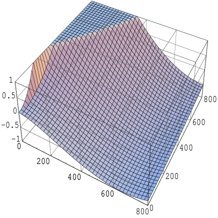
$M\,$ [MeV]

$M_{SS}\,$ [MeV]

Figure 2: $X_{1}^{8}({\rm large}\ M_{\eta^{\prime}})$ with $\Lambda=1$ GeV, as a function of $M$ and $M_{SS}$ in MeV.

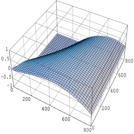
$M\,$ [MeV]

$M_{SS}\,$ [MeV]

Figure 4: $Y_{1}^{8}({\rm large}\ M_{\eta^{\prime}})$ with $\Lambda=1$ GeV, as a function of $M$ and $M_{SS}$ in MeV.

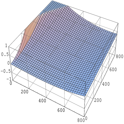
$M\,$ [MeV]

$M_{SS}\,$ [MeV]

Figure 6: $Y_{2}^{8}({\rm large}\ M_{\eta^{\prime}})$ with $\Lambda=1$ GeV, as a function of $M$ and $M_{SS}$ in MeV.

In Tables 1 to 6 and Table 8 we computed the one-loop corrections for various choices of the valence-meson mass $M$ and three values of the $\overline{MS}$ scale $\Lambda=1$ GeV, 770 MeV and 550 MeV. For $N=0$, we have set the parameters $\alpha$ and $\gamma^{8}_{12,}$ equal to zero, for simplicity. In Figs. 2, 4 and 6, we show the dependence of the three largest octet one-loop corrections, $X^{8}_{1}$ and $Y^{8}_{1,2}$ on $M$ and $M_{SS}$, for $N=2$ and large $M_{\eta^{\prime}}$. We do not show similar plots for $X^{8}_{2}$ and $Y^{27}$ because these one-loop corrections are typically much smaller. We also do not show a plot for ${\hat{X}}^{27}$, because it only depends on $M$ and not on $M_{SS}$, nor on any of the $\eta^{\prime}$ parameters.

These examples illustrate various points:

• One-loop corrections can be substantial, and will have to be taken into account in order to obtain a reliable estimate for $\alpha^{8}_{1,2}$ and $\alpha^{27}$ from the lattice. It may happen that the $O(p^{4})$ LECs have values such that the combined, scale independent contribution of $O(p^{4})$ non-analytic terms and counterterms are smaller than the non-analytic terms alone at a given scale $\Lambda\leq 1$ GeV, improving the convergence of ChPT. One would hope this to be the case, especially for ${\hat{X}}^{27}$, which is very large at the larger values of $M$ and $\Lambda$, and for $Y^{8}_{1}$ at larger $\Lambda$. This issue can be investigated on the lattice.

• The size of the one-loop corrections grows with increasing $\Lambda$. In particular, they are relatively small for $\Lambda=m_{\eta}\approx 550$ MeV. However, without further knowledge of $O(p^{4})$ LECs, it is unnatural to use $m_{\eta}$ as the scale, because the $\eta$ is itself a Goldstone boson, with mass very close to the meson masses we are considering here. In the absence of information on $O(p^{4})$ LECs, we believe that using higher values for $\Lambda$ gives a better a priori estimate of the size of $O(p^{4})$ effects. If, however, the values of $O(p^{4})$ LECs turn out to be such that $\Lambda=550$ MeV gives the better estimate, one-loop corrections would be reasonably small, and one-loop ChPT should be applicable in the computation of $\alpha^{8}_{1,2}$ and $\alpha^{27}$ from the lattice at realistic values of the quark masses.

• The fact that, in a number of cases, a one-loop correction becomes larger (and, in fact, diverges) with decreasing $M$ is a consequence of the fact that we do not vary $M_{SS}$ at the same time, i.e. of (partial) quenching. These “enhanced” chiral logarithms can be seen very clearly in the figures in the region $M<M_{SS}$, toward smaller $M$. Chiral logarithms are typically smaller near the line $M=M_{SS}$, for fixed $M+M_{SS}$. Enhanced chiral logarithms appear in all quantities except ${\hat{X}}^{27}$.

• So far, we have used the large-$M_{\eta^{\prime}}$ results, i.e. those of Subsect. 4.2, for all our examples. It is interesting to compare the $N\neq 0$ values obtained at a finite $\eta^{\prime}$ mass with those obtained for large $M_{\eta^{\prime}}$. In order to do this we chose $\delta=0.18$ for the finite-$M_{\eta^{\prime}}$ case. (In the real world $\delta\approx 0.18$; for quenched QCD $\delta\approx 0.1$ with a large error [25]). We set the other $\eta^{\prime}$-related parameters $\alpha$ and $\gamma^{8}_{1,2}$ equal to zero, simply because not much is known about their values (but see below for some remarks on contributions proportional to these parameters).

  For $N=2$, we show the difference between large and finite $M_{\eta^{\prime}}$ in Figs. 3, 5 and 7, for $X^{8}_{1}$ and $Y^{8}_{1,2}$. We show the ratios $[1+X({\rm finite}\ M_{\eta^{\prime}})]/[1+X({\rm large}\ M_{\eta^{\prime}})]$, with $X=X^{8}_{1},\,Y^{8}_{2}$, and the difference $Y^{8}_{1}({\rm finite}\ M_{\eta^{\prime}})-Y^{8}_{1}({\rm large}\ M_{\eta^{\prime}})$ (there is no tree-level contribution proportional to $\alpha^{8}_{1}$). The first thing to be noticed is that there are still enhanced chiral logarithms in the small $M$, large $M_{SS}$ region. This is because the coefficients of the enhanced chiral logarithms depend on $M_{\eta^{\prime}}$.

  In the small $M$, $M_{SS}$ region, the ratios are close to one (or, the difference is close to zero), as one would expect if both $M$ and $M_{SS}$ are small compared to $M_{\eta^{\prime}}$. For $N=2$, $M_{\eta^{\prime}}=863$ MeV, and $M^{2}_{SS}/M^{2}_{\eta^{\prime}}\approx 0.34$ for $M_{SS}=500$ MeV, while for $N=3$, $M_{\eta^{\prime}}=996$ MeV, so that $M^{2}_{SS}/M^{2}_{\eta^{\prime}}\approx 0.25$ for $M_{SS}=500$ MeV. We point out that for larger meson masses, the plots are less meaningful in the region $M>M_{SS}$. This is a consequence of the fact that we expanded the finite-$M_{\eta^{\prime}}$ results in $M^{2}/M^{2}_{\eta^{\prime}}$, but not in $M_{SS}^{2}/M^{2}_{\eta^{\prime}}$. This makes sense if $M<M_{SS}$, but not for $M\geq M_{SS}$. Therefore, for valence-quark masses close to the sea-quark mass, one either has to work consistently with the large-$M_{\eta^{\prime}}$ results, or a more general analysis using Eq. (3.4) instead of Eq. (3.8) is needed. The latter is outside the scope of the present paper, but for $M^{2}_{SS}/M^{2}_{\eta^{\prime}}\approx 0.25-0.34$ it appears reasonable to use the large-$M_{\eta^{\prime}}$ results of Subsect. 4.2.

  As a further illustration of this point, Table 7 shows the values of ${\cal M}^{2}$ and $A$ calculated from Eq. (3.8) (3rd, resp. 6th columns), the “exact” expression Eq. (3.4) with degenerate valence quark masses (4th and 7th columns), and in the limit of large $M_{\eta^{\prime}}$, Eq. (3.7) (5th and 8th columns). We see that the variation of values for ${\cal M}^{2}$ and $A$ is at most about 20, resp. 50%. This is not very large from a practical point of view: the current best determination of $m^{2}_{0}={\cal M}^{2}(N=0)$ in the quenched theory [25] has an error of the same order. We note that for $M=350$ MeV the values of ${\cal M}$ and $A$ are already much closer to their “exact” values ${\cal M}(M)$ and $A(M)$ than ${\cal M}_{\infty}$ and $A_{\infty}$.

  All this means that, for the value of parameters chosen in our examples, one could use the simplest possible form of the chiral logarithms, given in Subsect. 4.2, to fit numerical results. Tables 1 to 6 then give the relevant examples of the size of non-analytic one-loop corrections. Only with numerical results so precise that one would be able to determine ${\cal M}^{2}$ and $A$ with better precision would it be important to take the dependence on $\eta^{\prime}$ parameters into account. Note again that these conclusions do depend on the values of the meson masses (and hence quark masses) we considered in our examples.

• We also considered the effect of the $\eta^{\prime}$ couplings $\gamma^{8}_{1,2}$. They contribute to the octet matrix elements at one loop through the chiral logarithms $X^{\gamma}$ and $Y^{\gamma}_{1,2}$. In Table 8 we show the size of these one-loop corrections for the choice $\Lambda=1$ GeV. We see that these quantities are not very small, even though they vanish in the limit in which the $\eta^{\prime}$ decouples (for $N\neq 0$). They are typically smaller than $X^{8}_{1,2}$ and $Y^{8}_{1,2}$. If the couplings $\gamma^{8}_{1,2}$ themselves are small as well (compared to $\alpha^{8}_{1,2}$), it may be possible to ignore these terms. But if these couplings are not small, this would mean that the $\eta^{\prime}$ does play a role, even if we can use the large-$M_{\eta^{\prime}}$ partially-quenched expressions of Subsect. 4.2 for the other chiral logarithms.

  The results are not very sensitive to $\alpha$, except in the quenched case ($N=0$). We expect that, within the precision of current lattice computations, the effect of (arbitrarily) setting $\alpha$, as well as $\gamma^{8}_{1,2}$, to zero, can be accommodated in fits by shifts in the $O(p^{4})$ LECs $C^{8}_{V}$ etc. in Eq. (5), without significant impact on the values of the $O(p^{2})$ LECs $\alpha^{8}_{1,2}$ and $\alpha^{27}$. This can be checked by fitting lattice results while constraining these parameters to a few different values.

$X_{1}^{8}$

$R_{1}^{8}$

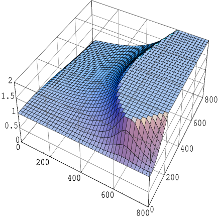
$M\,$ [MeV]

$M_{SS}\,$ [MeV]

Figure 3: $R^{8}_{1}=(1+X_{1}^{8}({\rm finite}\ M_{\eta^{\prime}}))/(1+X_{1}^{8}({\rm large}\ M_{\eta^{\prime}}))$ with $\Lambda=1$ GeV, as a function of $M$ and $M_{SS}$ in MeV.

$Y_{1}^{8}$

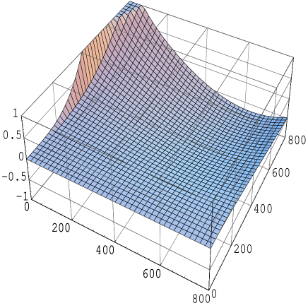
$M\,$ [MeV]

$M_{SS}\,$ [MeV]

Figure 5: $Y_{1}^{8}({\rm finite}\ M_{\eta^{\prime}})-Y_{1}^{8}({\rm large}\ M_{\eta^{\prime}})$ with $\Lambda=1$ GeV, as a function of $M$ and $M_{SS}$ in MeV.

$Y_{2}^{8}$

$R_{2}^{8}$

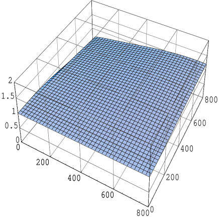
$M\,$ [MeV]

$M_{SS}\,$ [MeV]

Figure 7: $R^{8}_{2}=(1+Y_{2}^{8}({\rm finite}\ M_{\eta^{\prime}}))/(1+Y_{2}^{8}({\rm large}\ M_{\eta^{\prime}}))$ with $\Lambda=1$ GeV, as a function of $M$ and $M_{SS}$ in MeV.

6 Conclusion

We presented a complete analysis of $K\to\pi$ and $K\to 0$ weak matrix elements in one-loop ChPT for partially quenched QCD with $N$ degenerate sea quarks. For $K\to\pi$ we took the valence quarks degenerate in mass, while for $K\to 0$ they are kept non-degenerate in order to get a non-trivial result.

Three cases have been considered. The first is a partially quenched theory with a valence-meson mass much smaller than the $\eta^{\prime}$ mass, but with arbitrary value of $M_{SS}/M_{\eta^{\prime}}$, so that an expansion in powers of $M^{2}_{kk}/M^{2}_{\eta^{\prime}}$ is allowed. The second choice corresponds to the large $M_{\eta^{\prime}}$ limit where the $\eta^{\prime}$ decouples, so that we can also expand in $M^{2}_{SS}/M^{2}_{\eta^{\prime}}$. The third case is the quenched theory obtained for $N=0$ or $M_{SS}\to\infty$. For completeness, we also included results for the unquenched theory.

These results should be useful for extracting the values of the LECs $\alpha^{8}_{1,2}$ and $\alpha^{27}$ from Lattice QCD. As we emphasized already in the Introduction, these are interesting quantities in their own right. Estimates extracted from experiment exist, with which lattice results can be compared. The matrix elements considered here are the simplest weak matrix elements which can be used for this goal. The expressions to be used in fits to lattice data are given in Eq. (5), in which $X^{8}_{1,2}$, $X^{27}$, $Y^{8}_{1,2}$, $Y^{27}$, $X^{\gamma}$ and $Y^{\gamma}_{1,2}$ represent one-loop corrections (chiral logarithms), and $C^{8,27}_{V,S}$, $D^{8}_{V,S}$ and $D^{27}$ are linear combinations of $O(p^{4})$ LECs. They can be read off from the explicit one-loop results in Sects. (4.1-4).

From our numerical examples in Sect. 5 it is clear that one-loop expressions will be needed for typical values of quark masses used in present lattice computations. Contributions from $O(p^{4})$ operators, represented by the LECs $C^{8,27}_{V,S}$, $D^{8}_{V,S}$ and $D^{27}$, will also need to be included.

Theoretically, values for these $O(p^{4})$ LECs can also be extracted from lattice computations. However, realistically, we expect that such estimates would have large uncertainties, both as a consequence of the typical statistics of present lattice computations, as well as because of uncertainties related to the role of the $\eta^{\prime}$ discussed in more detail in Sect. 5. We note that the $O(p^{4})$ LEC $\beta^{27}_{1}$ can be accessed directly by a computation of the ratio of the $[K\to 0]_{27}$ and the $K^{0}-{\overline{K}}^{0}$-mixing matrix elements (cf. Eq. (5)).

In practice, for reasonably small values of the sea-quark mass (of order less than one-half times the strange-quark mass), it may be possible to use the partially quenched results for large $M_{\eta^{\prime}}$, given in Subsect. 4.2. In this case the $\eta^{\prime}$ decouples, and therefore all dependence on $\eta^{\prime}$ parameters, $m_{0}$, $\alpha$ and $\gamma^{8}_{1,2}$ is removed, making the analysis simpler. In addition, it is only in this limit that estimates obtained for $O(p^{4})$ LECs can be directly compared to those of the real world, provided that one chooses $N=3$ sea quarks. For a more detailed discussion, see Sects. 3 and 5. The more general results for the case that the sea-quark mass is larger, comparable to the $\eta^{\prime}$ mass, but the valence-quark mass is still small enough, are given in Subsect. 4.1.

A completely quenched lattice computation (for which the relevant results are in Subsect. 4.3) should be useful for assessing the feasibility of this approach. An $N=2$ computation, in combination with a quenched computation, could give insight into the dependence of the LECs on the number of light flavors. However, since we do not know the functional form of the $N$ dependence of the (finite part of the) LECs, an $N=3$ computation will be needed to obtain estimates without an uncontrolled systematic error.

The emphasis of this paper is on the extraction of reliable numbers for $\alpha^{8}_{1}$ and $\alpha^{27}$ from lattice computations. While these $O(p^{2})$ LECs are interesting, because of the availability of phenomenological estimates, the final aim of such Lattice QCD computations would be to convert these numbers into quantitative estimates of the $\Delta I=1/2$ and $\Delta I=3/2$ $K\to 2\pi$ decay amplitudes. This can be done using ChPT, and complete $O(p^{4})$ formulae for doing so are given in Ref. [19]. Assuming that $O(p^{4})$ ChPT is precise enough, the largest uncertainty arises because of the poor knowledge of all needed $O(p^{4})$ LECs. Many of these, as we discussed in Sect. 5, cannot even in principle be determined from the $K\to\pi$ and $K\to 0$ matrix elements. (More $O(p^{4})$ LECs are accessible through the $K^{0}-\overline{K}^{0}$ and $K\to 2\pi$ matrix elements with both pions at rest [8], the computation of which can also serve as a check on lattice results for $\alpha^{8}_{1}$ and $\alpha^{27}$.) One would have to resort either to the use of available phenomenological information [13], or to theoretical estimates based on arguments such as large $N_{c}$ or models (for recent discussions see Refs. [19, 26]).

In addition, it is well known that final-state interactions are responsible for a large enhancement of the $I=0$ $K\to\pi\pi$ amplitude [13, 27, 28]. In that case it could be necessary to resum those effects instead of relying on an $O(p^{4})$ ChPT calculation. A possible way of resumming final-state interactions has recently been proposed in Ref. [27].

Acknowledgements

We would like to thank Claude Bernard, Steve Sharpe as well as Akira Ukawa and other members of the CP-PACS collaboration for very useful discussions. MG would like to thank the Physics Departments of the Università “Tor Vergata,” Rome, the Universitat Autonoma, Barcelona, and the University of Washington, Seattle, for hospitality. MG is supported in part by the US Department of Energy, and EP by the Ministerio de Educaçion y Cultura of Spain.

References

- [1] L. Maiani, M. Testa, Phys. Lett. B245 (1990) 585
- [2] M. Golterman, K.C. Leung, Phys. Rev. D56 (1997) 2950
- [3] C. Bernard, T. Draper, G. Hockney, A. Soni, Nucl. Phys. B (Proc. Suppl.) 4 (1988) 483
- [4] S. Aoki et al. (JLQCD collaboration), Phys. Rev. D58 (1998) 054503
- [5] C. Dawson, G. Martinelli, G.C. Rossi, C. Sachrajda, S. Sharpe, M. Talevi, M. Testa, Nucl. Phys. B514 (1998) 313
- [6] M. Golterman, K.C. Leung, Phys. Rev. D58 (1998) 097503
- [7] M. Golterman, E. Pallante, Nucl. Phys. B (Proc. Suppl.) 83-84 (2000) 250
- [8] M. Golterman, E. Pallante, in progress
- [9] L. Lellouch, M. Lüscher, hep-lat/0003023
- [10] C. Bernard, T. Draper, A. Soni, H. Politzer, M. Wise, Phys. Rev. D32 (1985) 2343
- [11] J. Kambor, J. Missimer, D. Wyler, Nucl. Phys. B346 (1990) 17
- [12] E. Pallante, JHEP 01 (1999) 012
- [13] J. Kambor, J. Missimer, D. Wyler, Phys. Lett. B261 (1991) 496; Phys. Rev. Lett. 68 (1992) 1818.
- [14] C. Bernard, M. Golterman, Phys. Rev. D49 (1994) 486
- [15] A. Morel, J. Physique 48 (1987) 111
- [16] C. Bernard, M. Golterman, Phys. Rev. D46 (1992) 853
- [17] G. Ecker, J. Kambor and D. Wyler, Nucl. Phys. B394 (1993) 101
- [18] J. Gasser, H. Leutwyler, Nucl. Phys. B250 (1985) 465
- [19] J. Bijnens, E. Pallante, J. Prades, Nucl. Phys. B521 (1998) 305
- [20] M. Golterman, K.C. Leung, Phys. Rev. D57 (1998) 5703
- [21] S. Sharpe, Nucl. Phys. B (Proc. Suppl.) 17 (1990) 146
- [22] S. Sharpe, Phys. Rev. D46 (1992) 3146
- [23] S. Sharpe, Phys. Rev. D56 (1997) 7052; S. Sharpe and N. Shoresh, Nucl. Phys. B (Proc. Suppl.) 83-84 (2000) 968; hep-lat/0006017
- [24] G. Colangelo, E. Pallante, Nucl. Phys. B520 (1998) 433.
- [25] S. Aoki et al. (CP-PACS collaboration), Phys. Rev. Lett. 84 (2000) 238; W. Bardeen, A. Duncan, E. Eichten, H. Thacker, Nucl. Phys. B (Proc. Suppl.) 83-84 (2000) 215
- [26] J. Bijnens, J. Prades, JHEP 0001 (2000) 002
- [27] E. Pallante, A. Pich, Phys. Rev. Lett. 84 (2000) 2568
- [28] T.N. Truong, Phys. Lett. B207 (1988) 495; A.A. Belkov et al., Phys. Lett. B220 (1989) 459; N. Isgur et al., Phys. Rev. Lett. 64 (1990) 161; Nucl. Phys. A508 (1990) 371c; M. Neubert, B. Stech, Phys. Rev. D44 (1991) 775.