Abstract

We report on a study of the supersymmetric anharmonic oscillator computed using a euclidean lattice path integral. Our numerical work utilizes a Fourier accelerated hybrid Monte Carlo scheme to sample the path integral. Using this we are able to measure massgaps and check Ward identities to a precision of better than one percent. We work with a non-standard lattice action which we show has an exact supersymmetry for arbitrary lattice spacing in the limit of zero interaction coupling. For the interacting model we show that supersymmetry is restored in the continuum limit without fine tuning. This is contrasted with the situation in which a ‘standard’ lattice action is employed. In this case supersymmetry is not restored even in the limit of zero lattice spacing. Finally, we show how a minor modification of our action leads to an exact, local lattice supersymmetry even in the presence of interaction.

Introduction

Supersymmetry is thought to be a crucial ingredient in any theory which attempts to unify the separate interactions contained in the standard model of particle physics. Since low energy physics is manifestly not supersymmetric it is necessary that this symmetry be broken at some energy scale. Issues of spontaneous symmetry breaking have proven difficult to address in perturbation theory and hence one is motivated to have some non-perturbative method for investigating such theories. The lattice furnishes such a framework. Unfortunately, supersymmetry being a spacetime symmetry is explicitly broken by the discretization procedure and it is highly non-trivial problem to show that it is recovered in the continuum limit.

One manifestation of this problem is the usual doubling problem of lattice fermions - the naive fermion action in $D$ dimensions possesses not one but $2^{D}$ continuum-like modes. These extra modes persist in the continuum limit and yield an immediate conflict with supersymmetry requiring as it does an equality between boson and fermion degrees of freedom. As has been noted by several authors [1] it is possible to circumvent this problem in a free theory by the addition of a simple Wilson mass term to the fermion action. This removes the doubles and leads to a supersymmetric free theory in the continuum limit. However such a procedure fails when interactions are introduced. Instead we shall show that the use of a non-standard lattice action allows the quantum continuum limit of such an interacting theory to admit continuum supersymmetry [2]. Indeed, we will show that this action has an exact lattice supersymmetry in the absence of interactions (similar to that proposed in [3]) and very small symmetry breaking effects at non-zero interaction coupling. Finally, we write down an action for the interacting theory which is supersymmetric for all lattice spacings.

Model

The model we will study contains a real scalar field $x$ and two independent real fermionic fields $\psi$ and $\overline{\psi}$ defined on a one-dimensional lattice of $L$ sites with periodic boundary conditions imposed on both scalar and fermion fields.

$$S=\sum_{ij}\frac{1}{2}\left[-x_{i}D^{2}_{ij}x_{j}+\overline{\psi}_{i}\left(D_{ij}+P^{\prime}_{ij}\right)\psi_{j}\right]+\sum_{i}\frac{1}{2}P_{i}^{2}$$ (1)

The quantity $P_{i}$ is defined as

$$P_{i}=\sum_{j}K_{ij}x_{j}+gx_{i}^{3}$$

and its derivative is then just

$$P^{\prime}_{ij}=K_{ij}+3gx_{i}^{2}\delta_{ij}$$

The choice of a cubic interaction term in $P(x)$ guarantees unbroken supersymmetry [4] in the continuum. The matrix $D_{ij}$ is the symmetric difference operator

$$D_{ij}=\frac{1}{2}\left[\delta_{j,i+1}-\delta_{j,i-1}\right]$$

and $K_{ij}$ is the Wilson mass matrix

$$K_{ij}=m\delta_{ij}-\frac{r}{2}\left(\delta_{i,j+1}+\delta_{i,j-1}-2\delta_{ij}\right)$$

We work in dimensionless lattice units in which $m=m_{\rm phys}a$, $g=g_{\rm phys}a^{2}$ and $x=a^{-\frac{1}{2}}x_{\rm phys}$.

Notice that the boson operator $D^{2}$ is not the usual lattice Laplacian $\Box=D_{+}D_{-}$ but contains a double corresponding to the extra zero in $D=\frac{1}{2}(D_{+}+D_{-})$. However, the boson action contains now a Wilson mass term and so this extra state, like its fermionic counterpart, decouples in the continuum limit. With the further choice $r=1$ the fermion matrix $M=D+P^{\prime}$ is almost lower triangular and its determinant can be shown to be

$${\rm det}(M)=\prod_{i=1}^{L}\left(1+m+3gx_{i}^{2}\right)-1$$

which is positive definite for $g>0$ and $m>0$. This fact will be utilized in our numerical algorithm. Furthermore, the choice $r=1$ removes the doubles completely in the free theory and renders the fermion correlators simple exponentials.

Simulation

In order to simulate the fermionic sector we first replace the fermion field by a bosonic pseudofermion field $\phi$ whose action is just

$$\sum_{ij}\frac{1}{2}\phi_{i}\left(M^{T}M\right)^{-1}_{ij}\phi_{j}$$

This is an exact representation of the original fermion effective action provided the determinant of the fermion matrix is positive definite. The resultant (non-local) action $S\left(x,\phi\right)$ can now be simulated using the Hybrid Monte Carlo (HMC) algorithm [5]. In the HMC scheme momentum fields $(p,\pi)$ conjugate to $(x,\phi)$ are added and a Hamiltonian $H$ defined which is just the sum of the original action plus additional terms depending on the momenta $H=S+\Delta S$.

$$\Delta S=\sum_{i}\frac{1}{2}\left(p_{i}^{2}+\pi_{i}^{2}\right)$$

On integrating out the momenta it is clear that this partition function is (up to a constant) identical to the original one. The augmented system $(x,p,\phi,\pi)$ is now naturally associated with some classical dynamics depending on an auxiliary time variable $t$

$$\frac{\partial x}{\partial t} = p$$

$$\frac{\partial p}{\partial t} = -\frac{\partial H}{\partial x}$$

$$\frac{\partial\phi}{\partial t} = \pi$$

$$\frac{\partial\pi}{\partial t} = -\frac{\partial H}{\partial\phi}$$

If we introduce a finite time step $\Delta t$ we may simulate this classical evolution and produce a sequence of configurations $(x(t),\phi(t))$. If $\Delta t=0$ then $H$ would be conserved along such a trajectory. In practice $\Delta t$ is finite and $H$ is not exactly conserved. However a finite length of such an approximate trajectory can still be used as a global move on the fields $(x,\phi)$ which may then be subject to a Metropolis step based on $\Delta H$. Provided the classical dynamics is reversible and care is taken to ensure ergodicity the resulting move satisfies detailed balance and hence this dynamics will provide a simulation of the original partition function. The reversibility criterion can be satisfied by using a leapfrog integration scheme and ergodicity is taken care of by drawing new momenta from a Gaussian distribution after each such trajectory.

If we introduce bosonic and pseudofermionic forces

$$F_{i}(t)=-\frac{\partial H(t)}{\partial x_{i}}$$ (2)

and

$${\mathcal{F}}_{i}(t)=-\frac{\partial H(t)}{\partial\phi_{i}},$$ (3)

the resultant evolution equations look like

$$x_{i}(t+\Delta t) = x_{i}(t)+\Delta tp_{i}(t)-\frac{(\Delta t)^{2}}{2}F_{i}(t)$$

$$\phi_{i}(t+\Delta t) = \phi_{i}(t)+\Delta t\pi_{i}(t)-\frac{(\Delta t)^{2}}{2}{\mathcal{F}}_{i}(t)$$

$$p_{i}(t+\Delta t) = p_{i}(t)+\frac{\Delta t}{2}\left(F_{i}(t)+F_{i}(t+\Delta t)\right)$$

$$\pi_{i}(t+\Delta t) = \pi_{i}(t)+\frac{\Delta t}{2}\left({\mathcal{F}}_{i}(t)+{\mathcal{F}}_{i}(t+\Delta t)\right)$$ (4)

The force terms are then given in terms of a vector $s_{i}$ which is a solution of the (sparse) linear problem

$$\left(M^{T}M\right)_{ij}s_{j}=\phi_{i}$$

$$\frac{\partial H}{\partial x_{i}} = -D^{2}_{ij}x_{j}+P^{\prime}_{ij}P_{j}+6gx_{i}s_{i}M_{ij}s_{j}$$

$$\frac{\partial H}{\partial\phi_{i}} = s_{i}$$

In order to reduce the effects of critical slowing down we have chosen to perform this update in momentum space using FFTs and a momentum dependent time step. Thus, for example, the lattice field $x_{m},(m=0\ldots L-1$) can be expanded as

$$x_{m}=\sqrt{\frac{1}{L}}\sum_{n}\overline{x}_{n}e^{i\frac{2\pi mn}{L}}$$

where $\overline{x}_{n}$ is the Fourier amplitude with wavenumber $\frac{2\pi}{L}n$ ($n=0\ldots L-1$) and the Fourier amplitudes $\overline{x}_{n}$ are updated using equations 4 with $\Delta t=\Delta t(n)$. For the boson field $x$ we use $\Delta t=\tau_{B}$ where

$$\tau_{B}(n)=\epsilon\frac{\left(m_{\rm eff}+2r\right)}{\sqrt{\sin^{2}{\frac{2\pi n}{L}}+\left(m_{\rm eff}+2r\sin^{2}{\frac{2\pi n}{2L}}\right)^{2}}}$$

For the pseudofermion field update we use the inverse function $\Delta t=\tau_{F}=\frac{1}{\tau_{B}}$. With these choices (and $m_{\rm eff}=ma$) it is simple to show that the $g=0$ theory suffers no critical slowing down - all modes are updated at the same rate independent of their wavelength. By setting $m_{\rm eff}$ at the approximate position of the massgap in the interacting case we have found very substantial reductions in the autocorrelation time for the two point functions of the theory. In practice we set $\epsilon\sim 0.1$ and the number of leapfrog integrations per trajectory at $N_{\rm leap}=10$.

Correlation functions

We have measured the following correlators

$$G^{B}_{ij}=\left<x_{i}x_{j}\right>$$

and

$$G^{F}_{ij}=\left<s_{j}M_{ik}s_{k}\right>$$

It can be shown that the latter is simply an estimator for the original fermion correlator $<\overline{\psi}_{i}\psi_{j}>$.

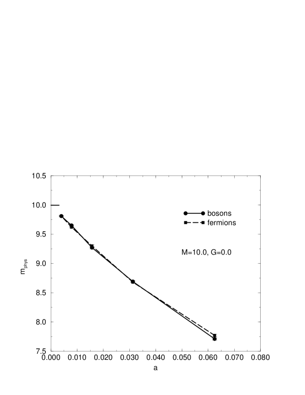
Figure 1: Boson and Fermion masses vs. lattice spacing $a$ at $m_{\rm phys}=10.0$, $g_{\rm phys}=0.0$

In figure 1 we show first the results of a simulation of this model for $g_{\rm phys}=0.0$ and $m_{\rm phys}=10.0$. The data set consists of $10^{6}$ Fourier accelerated HMC trajectories. The plot shows both boson and fermion massgaps, extracted from a simple exponential fit to the correlators over the first $L/4$ timeslices, as a function of the lattice spacing $a=1/L$. Notice that boson and fermion masses while receiving large O(a) systematic errors (due to the Wilson term) are degenerate within statistical errors. We see furthermore that as ${\rm a}\to 0$ the common massgap approaches the correct continuum value. As we shall see later the free action has an exact supersymmetry at finite lattice spacing which is responsible for the boson/fermion degeneracy.

Figure 2: Boson and Fermion masses vs. lattice spacing $a$ at $m_{\rm phys}=10.0$, $g_{\rm phys}=100.0$

We have also examined the massgaps at non-zero coupling. Figure 2 shows the same plot for $m_{\rm phys}=10.0$ and $g_{\rm phys}=100.0$. The massgaps are also listed in Table 1.

L	$m_{B}$	$m_{F}$
16	$10.60(3)$	$10.64(5)$
32	$12.80(2)$	$12.91(4)$
64	$14.47(2)$	$14.52(2)$
128	$15.63(4)$	$15.63(4)$
256	$16.19(3)$	$16.28(4)$

Table 1: Boson and Fermion massgaps for $g/m^{2}=1$ versus inverse lattice spacing

The data set consists of $10^{6}$ trajectories again using lattice sizes $L=16-256$. The effective dimensionless expansion parameter is $g/m^{2}$ so this corresponds to a regime of strong coupling. Remarkably, the boson and fermion masses are again degenerate within statistical errors O($0.5$%) and flow as ${\rm a}\to 0$ to the correct continuum limit (the latter can be computed easily using Hamiltonian methods and yields $m_{\rm cont}=16.87$)). That this result is nontrivial can be seen when we compare it to the result of a ‘naive’ discretization of the continuum action using $\Box$ in place of $D^{2}$ and the usual Wilson action for the fermions – figure 3.

Figure 3: Boson and Fermion masses vs. lattice spacing $a$ at $m_{\rm phys}=10.0$, $g_{\rm phys}=100.0$ computed from ‘naive’ action

In this case the mass plot looks very different. At large lattice spacing the extracted massgaps differ widely – the fermion having O(a) errors while the boson is much smaller (it varies as O(${\rm a}^{2}$) at $g=0$). Initially they appear to approach each other as ${\rm a}\to 0$ but the two curves depart for fine lattice spacing and do not approach the correct continuum limit - the quantum continuum limit is not supersymmetric. Thus naive discretizations of the continuum action will break supersymmetry irreversibly even in theories such as quantum mechanics which have no divergences. At minimum it would be necessary to tune parameters to obtain a supersymmetric continuum limit. In comparison the numerical results of figure 2 indicate that supersymmetry breaking effects, if present, are very small. We examine this more carefully next.

Supersymmetry

Motivated by the form of the continuum supersymmetry transformations for this model consider the following two lattice transformations

$$\delta_{1}x_{i} = \overline{\psi_{i}}\xi$$

$$\delta_{1}\psi_{i} = \left(D_{ij}x_{j}-P_{i}\right)\xi$$

$$\delta_{1}\overline{\psi_{i}} = 0$$ (5)

and

$$\delta_{2}x_{i} = \psi_{i}\overline{\xi}$$

$$\delta_{2}\psi_{i} = 0$$

$$\delta_{2}\overline{\psi_{i}} = \left(D_{ij}x_{j}+P_{i}\right)\overline{\xi}$$ (6)

where $\xi$ and $\overline{\xi}$ are independent anti-commuting parameters. The existence of two such symmetries reflects the $N=2$ character of the continuum supersymmetry. If we perform the variation corresponding to the first of these (eqn. 5) we find

$$\delta_{1}S=\sum_{i}\overline{\psi}_{i}\xi\left(P^{\prime}_{ij}D_{jk}x_{k}-D_{ij}P_{j}\right)$$ (7)

The expression corresponding to the second transformation eqn. 6 is similar

$$\delta_{2}S=\sum_{i}\overline{\xi}\psi_{i}\left(P^{\prime}_{ij}D_{jk}x_{k}-D_{ij}P_{j}\right)$$ (8)

In the continuum limit $a=0$ the difference operators become derivatives and the term inside the brackets is zero - this is the statement of continuum supersymmetry. Notice, for $g=0$ and $a\neq 0$ this term is still zero - the classical free lattice action is also supersymmetric. However this term is non-zero for finite spacing and non-zero interaction coupling - the classical lattice action breaks supersymmetry. Since we use the symmetric difference operator this breaking will be ${\rm O}(gL^{-2})$. From the point of view of a continuum limit such a breaking would not be important - since the theory contains no divergences all non-supersymmetric terms induced in the quantum effective action will have couplings that vanish as $a\to 0$. Indeed, as was shown explicitly in [2], the two-dimensional Wess-Zumino model has a supersymmetric continuum limit when regulated in this way. For a lattice of size $L=16$ and $g_{\rm phys}=100.0$ we would expect symmetry breaking terms to be suppressed by a factor of $g_{\rm phys}/L^{4}=0.002$. This is consistent with what we see in the massgaps.

To verify these conclusions we have studied the approximate Ward identities which follow from the lattice transformations eqn. 5 and eqn. 6.

Ward identities

The Ward identities corresponding to these approximate symmetries can be derived in the usual way. First consider the partition function with external sources

$$Z\left(J,\theta,\overline{\theta}\right)=\int DxD\psi D\overline{\psi}e^{-S+\sum J.x+\overline{\theta}.\psi+\theta.\overline{\psi}}$$

Perform a lattice supersymmetry transformation, for example, eqn. 5. The action $S$ varies as in eqn. 7, and the integration measure is invariant while the source terms vary. Since the partition function does not change (the transformation can be viewed as a change of variables) we find

$$0=\delta Z=\int DxD\psi D\overline{\psi}e^{-S}\left(\sum J.\delta x+\overline{\theta}.\delta\psi+\theta.\delta\overline{\psi}+\alpha.\overline{\psi}\right)$$ (9)

where $\alpha_{i}=\left(P^{\prime}_{ij}D_{jk}x_{k}-D_{ij}P_{j}\right)$ Furthermore, any number of derivatives with respect to the sources evaluated for zero sources will also vanish. For the first supersymmetry equation 5 this yields a set of identities connecting different correlation functions. The first non-trivial example is

$$\left<\overline{\psi_{i}}\psi_{j}\right>+\left<(D_{jk}x_{k}-P_{j})x_{i}\right>+\left<\alpha_{k}\overline{\psi}_{k}x_{i}\psi_{j}\right>=0$$

The last term represents the symmetry breaking term which may be rewritten as $<(M^{T})^{-1}_{jk}\alpha_{k}x_{i}>$. Since $\alpha_{k}$ is a vector with random elements each of mean zero and suffering fluctuations O($g/L^{2})$) we might expect that this term contributes rather a small correction to the Ward identity. In this spirit we will neglect it at this point and see if the predictions are substantiated by the results of the simulation. It is important to notice that this correction to the naive Ward identity is finite (quantum mechanics) and multiplied by $1/L^{2}$ and consequently the continuum limit is guaranteed to possess supersymmetry. The same will be true for any approximate Ward identity we care to construct.

A second Ward identity may be derived corresponding to the second (approximate) supersymmetry equation 6 we find

$$\left<\psi_{i}\overline{\psi_{j}}\right>+\left<(D_{jk}x_{k}+P_{j})(x)x_{i}\right>=0$$

More conveniently we can add and subtract these equations to yield the relations

$$G^{F}_{ij}-G^{F}_{ji}=-\left<2D_{jk}x_{k}x_{i}\right>$$ (10)

and

$$G^{F}_{ij}+G^{F}_{ji}=\left<2P_{j}x_{i}\right>$$ (11)

Translation invariance on the lattice implies $G^{F}_{ij}=G^{F}(t)$ and $G^{F}_{ji}=G^{F}(L-t)$ where $t=(j-i)$. We can check that these two Ward identities are satisfied numerically by forming the two (distance dependent) quantities $w_{1}$ and $w_{2}$ which are defined by

$$w_{1}\left(t\right)=\frac{G^{F}_{ij}+G^{F}_{ji}-2\left<x_{i}P_{j}\right>}{2\left<x_{i}P_{j}\right>}$$ (12)

$$w_{2}\left(t\right)=\frac{G^{F}_{ij}-G^{F}_{ji}+2\left<x_{i}D_{jk}x_{k}\right>}{2\left<x_{i}D_{jk}x_{k}\right>}$$ (13)

Figure 4: $w_{1}(t)$ vs. $t$ for $L=16$, $m_{\rm phys}=10.0$ and $g_{\rm phys}=0.0$

Figure 5: $w_{2}(t)$ vs. $t$ for $L=16$, $m_{\rm phys}=10.0$ and $g_{\rm phys}=0.0$

These are shown in figure 4 and figure 5 for a lattice of size $L=16$ at $g_{\rm phys}=0.0$. In this case we expect the symmetry to be exact and indeed we see that the Ward identities are satisfied within statistical accuracy.

Figures 6 and 7 show plots of $w_{1}$ and $w_{2}$ for a lattice of size $L=16$ at $g_{\rm phys}=100.0$. It is clear that within our statistical error (on the order of a few percent for these quantities) we are again not sensitive to the SUSY breaking terms and the continuum Ward identities are satisfied.

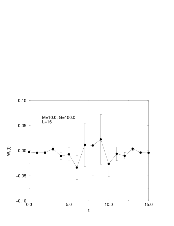
Figure 6: $w_{1}(t)$ vs. $t$ for $L=16$,$m_{\rm phys}=10.0$ and $g_{\rm phys}=100.0$

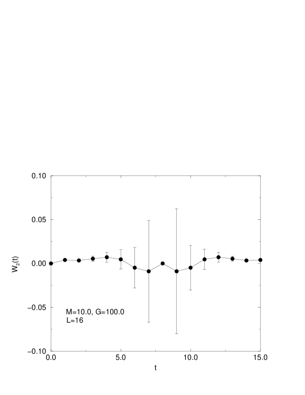
Figure 7: $w_{2}(t)$ vs. $t$ for $L=16$, $m_{\rm phys}=10.0$ and $g_{\rm phys}=100.0$

Discussion and Conclusions

We have performed a numerical study of the lattice supersymmetric anharmonic oscillator computed using path integrals. This is essentially a one-dimensional version of the Wess-Zumino model. We have utilized a lattice discretization which preserves two exact supersymmetries in the free theory. We are able to show that the interacting theory flows to a supersymmetric fixed point in the zero lattice spacing limit without fine tuning. This is to be contrasted with naive discretizations of the continuum action which require fine tuning to recover supersymmetry in the continuum limit.

Furthermore, we have estimated the magnitude of supersymmetry breaking at O($g/L^{2}$) which is typically smaller than one percent even at strong coupling and for coarse lattices. Thus the lattice simulations are, in practice, very close to the supersymmetric fixed point. We have checked the first two non-trivial Ward identities following from this (approximate) invariance. Our numerical results place an upper bound on the magnitude of symmetry breaking corrections which is consistent with this estimate.

It is tempting to try to interpret the numerical results as evidence of an exact lattice supersymmetry even in the presence of interactions. Using the antisymmetry of the derivative operator it is easy to show that the symmetry breaking term 8 can be rewritten

$$\delta_{2}S=\delta_{2}\sum x_{i}D_{ij}P_{j}$$

Thus $S_{\rm new}=S-\sum x_{i}D_{ij}P_{j}$ will be exactly invariant under the second lattice supersymmetry transformation even for non zero interaction. Notice that the presence of an extra minus sign prevents this new action from having a second invariance corresponding to the first supersymmetry 7. This invariant action can be rewritten in the form

$$S_{\rm new}=\sum_{ij}\frac{1}{2}\left(D_{ij}x_{j}+P_{i}\right)\left(D_{ij}x_{j}+P_{i}\right)+\sum_{ij}\overline{\psi}_{i}\left(D_{ij}+P^{\prime}_{ij}\right)\psi_{j}$$

This allows us to identify the Nicolai map for the model [6]. The latter is the non-trivial transformation $x_{i}\to\xi_{i}$ which maps the boson action to a free field form and whose Jacobian simultaneously cancels the fermion determinant. Here we see it explicitly

$$\xi_{i}=D_{ij}x_{j}+P_{i}$$

It has previously been pointed out that the identification of such a map may be used to help find lattice supersymmetric actions [7] and [8]. This quantum mechanics model furnishes a concrete example - the lattice action which admits the Nicolai map is invariant under a transformation which interchanges bosonic and fermionic degrees of freedom. In the continuum limit this lattice action approaches its continuum counterpart and the transformation reduces to a continuum supersymmetry transformation. The presence of one exact supersymmetry is already enough to guarantee vanishing vacuum energy and boson/fermion mass degeneracy for the lattice theory.

It would be interesting to extend these calculations to the two-dimensional Wess-Zumino model and verify non-perturbatively the results derived perturbatively in [2].

References

-
[1]
Hiroto So and Naoya Ukita, Phys.Lett. B457 (1999) 314
Tatsumi Aoyama and Yoshio Kikukawa, Phys.Rev. D59 (1999) - [2] M. Goltermaan and D. Petcher, Nucl. Phys. B319 (1989) 307.
- [3] W. Bietenholz, Mod. Phys. Lett A14 (1999) 51.
- [4] E. Witten, Nucl. Phys. B185 (1981) 513.
- [5] S. Duane, A. Kennedy, B. Pendleton and D. Roweth, Phys. Lett. B195B (1987) 216.
- [6] H. Nicolai, Phys. Lett. B89 (1980) 341.
- [7] N. Sakai and M. Sakamoto, Nucl. Phys. B229 (1983) 173.
- [8] M. Beccaria, G. Curci and E. D’Ambrosio, Phys. Rev. D58 (1998) 065009.