The finite temperature QCD phase transition with domain wall fermions

Abstract

The domain wall formulation of lattice fermions is expected to support accurate chiral symmetry, even at finite lattice spacing. Here we attempt to use this new fermion formulation to simulate two-flavor, finite temperature QCD near the chiral phase transition. In this initial study, a variety of quark masses, domain wall heights and domain wall separations are explored using an $8^{3}\times 4$ lattice. Both the expectation value of the Wilson line and the chiral condensate show the temperature dependence expected for the QCD phase transition. Further, the desired chiral properties are seen for the chiral condensate, suggesting that the domain wall fermion formulation may be an effective approach for the numerical study of QCD at finite temperature.

I Introduction

Many of the properties of low energy QCD are a direct consequence of the breaking of chiral symmetry by the QCD vacuum. It is expected that this spontaneous chiral symmetry breaking will disappear as the temperature is increased. Both the nature of this symmetry restoration (abrupt phase transition or continuous cross-over) and the character of the high-temperature quark-gluon plasma phase are active areas of both theoretical[1, 2] and experimental research[3, 4].

An especially promising approach to the theoretical study of equilibrium properties of both the QCD phase transition and the high-temperature plasma phase is direct numerical simulation of the Feynman path integral using the methods of lattice gauge theory. The quantum partition function is written as a Euclidean path integral that can be studied ab initio using the discrete, lattice formulation of Wilson[5]. While the local color gauge symmetry of the theory remains exact at any lattice spacing in Wilson’s formulation, much of the theory’s flavor symmetry, and especially its chiral component, is explicitly broken.

This difficulty in representing the continuum flavor symmetries in a lattice fermion formulation is a serious problem that has persisted for more than two decades. When the fermion action is naively discretized the low-energy fermionic degrees of freedom increase by a factor of $2^{4}$. This well-known “doubling” problem can only be remedied by methods that explicitly break the chiral flavor symmetries for finite lattice spacing [6]. The chiral symmetries are then recovered together with the Lorentz symmetry as the lattice spacing is sent to zero. The most popular of these methods are staggered[7, 8, 9] and Wilson[5] fermions.

Although, in principle these methods should be able to approximate the continuum theory in a controlled way, in practice this problem has been a formidable obstacle to lattice studies of the QCD phase transition. For example, the Wilson fermion formulation explicitly breaks all of the continuum chiral symmetries making phenomena driven by the spontaneous breakdown of chiral symmetry difficult to study. While staggered fermions do possess a one-dimensional continuous chiral symmetry at finite lattice spacing, this formulation explicitly breaks the vector flavor symmetry so instead of three light Goldstone pions with mass on the order of the critical temperature $T_{c}\approx 160$ MeV as found in Nature, present staggered simulations have masses for two of the three pions in the range 500-600 GeV, certainly too large.

In addition, the subtle effects of the continuum axial anomaly which are closely connected with the order of the transition[10] are badly mutilated by both fermion formalisms at finite lattice spacing. While the anomalous $U_{A}(1)$ continuum chiral symmetry is explicitly broken by both formalisms, the fermion zero modes required by Atiyah-Singer index theorem are shifted away from zero by finite lattice spacing effects.

In principle, each of these difficulties can be addressed by simply working at smaller lattice spacing. However, present numerical methods scale very poorly as the lattice spacing is decreased, with the required numerical effort growing as $\sim 1/a^{8-10}$ for lattice spacing $a$.

Domain wall fermions (DWF) offer a new approach to the problem of including fermions in lattice gauge theory calculations. In this formulation, introduced by Kaplan [11, 12], the fermionic fields are defined on a five-dimensional hyper-cubic lattice using a local action. The fifth direction can be thought of as an extra space-time dimension or as a new internal flavor space. The gauge fields are represented in the standard way in four dimensional space-time and are coupled to the extra fermion degrees of freedom in a diagonal fashion.

In this paper, we use a variant of Kaplan’s approach, developed by Shamir[13], in which the two four-dimensional faces orthogonal to the new fifth dimension are treated differently, with free boundary conditions imposed on the fermion fields. This key ingredient allows a system made up of naively massive fermions to develop chiral surface states on these boundaries (domain walls) with the positive chirality states bound exponentially to one wall and the negative chirality states bound to the other.

The two chiralities overlap only by an amount that is exponentially small in $L_{s}$, the number of lattice sites along the fifth direction. The resulting mixed state forms a Dirac 4-spinor that propagates in the four-dimensional space-time with an exponentially small mass. Therefore, the amount of chiral symmetry breaking that is artificially induced by the regulator can be controlled by the new parameter $L_{s}$. In the $L_{s}\rightarrow\infty$ limit the chiral symmetry is exact even at finite lattice spacing. Thus, the domain wall fermion method has succeeded in disentangling the chiral limit ($L_{s}\rightarrow\infty$) and the continuum limit ($a\rightarrow 0$). Furthermore, the direct computing requirement grows only linearly with $L_{s}$.

Here we report the first full QCD simulations using domain wall fermions in four dimensions. The properties and parameter space of domain wall fermions appropriate for a study of QCD thermodynamics are explored in detail. Small lattices of size $8^{3}\times 4$ were used to perform numerical simulations of full, two-flavor QCD at finite temperature. Preliminary results of this work have appeared in [14, 15, 16]. These studies have been carried out using the QCDSP supercomputer at Columbia[17]. Based on the work reported here, results of physical interest have been obtained on larger lattices for a variety of observables. Preliminary results of these studies can be found in [14, 16] and will be presented in follow-on papers[18].

For a detailed introduction to the subject and relevant references the reader is referred to Refs. [19, 20, 21], and the reviews in Refs. [22, 23, 24, 25]. Earlier numerical work using domain wall fermions has explored the parameter space of a QCD-like, dynamical vector theory in two dimensions, the two flavor Schwinger model[19, 20]. For applications to quenched QCD see Refs. [26, 27, 28, 29, 30, 31, 32, 33, 34, 35, 36, 37, 15] for applications to four-Fermi models see Ref. [38] and for possible alternatives to domain wall fermion simulations see Refs. [39, 40, 41, 42, 43, 44, 45].

In Section II the action of the theory and a brief description of the numerical methods are presented. In Section III some important analytical facts are outlined in order to help guide the numerical investigation. In Section IV we study the chiral properties of the theory both below and above the chiral phase transition. Our numerical results suggest that domain wall fermions are able to sustain the desired chiral properties of QCD, even at finite lattice spacing. Both a low temperature phase where the $SU(2)\times SU(2)$ chiral symmetry is broken spontaneously to an $SU(2)$ vector symmetry and a high temperature phase where the full $SU(2)\times SU(2)$ chiral symmetry is intact can be recognized.

In Section IV the dependence on the two new regulator parameters, the number of sites in the fifth direction $L_{s}$, and the domain wall “height” $m_{0}$, is studied numerically. Finally, in Section VI conclusions and outlook are presented. Appendix A gives the explicit form of the gamma matrices used in this work while Appendix B describes the molecular dynamics equations of motion. Tables summarizing the numerical results are given at the end of the paper.

II Hybrid Monte Carlo with domain wall fermions

In this section the action of QCD with domain wall fermions, its implementation for the Hybrid Monte Carlo (HMC) algorithm, and the parameters used in the simulations are described. In the following, we discuss the case of two degenerate flavors implemented using the HMC $\Phi$ algorithm[46]. (An odd number of flavors can be simulated using the HMC $R$ algorithm[46]).

Domain wall fermions can be used in numerical simulations in a fashion similar to traditional Wilson fermions. In fact, if the fifth direction is thought of as an internal flavor direction then an HMC simulation with DWF is identical to a simulation of many flavors of Wilson fermions with a sophisticated mass matrix. We use the partition function of QCD with domain wall fermions proposed in [47] but with a slightly different heavy flavor subtraction as in [19, 20]. In particular:

$$Z=\int[dU]\int[d\overline{\Psi}d\Psi]\int[d\Phi_{PV}^{\dagger}d\Phi_{PV}]e^{-S}$$ (1)

$U_{\mu}(x)$ is the gauge field, $\Psi(x,s)$ is the fermion field and $\Phi_{PV}(x,s)$ is a bosonic, Pauli-Villars field. The variable $x$ specifies the coordinates in the four-dimensional space-time box with extent $L$ along each of the spatial directions and extent $N_{t}$ along the time direction while $s=0,1,\dots,L_{s}-1$ is the coordinate of the fifth direction, with $L_{s}$ assumed to be even. The action $S$ is given by:

$$S=S_{G}(U)+S_{F}(\overline{\Psi},\Psi,U)+S_{PV}(\Phi_{PV}^{\dagger},\Phi_{PV},U)$$ (2)

where:

$$S_{G}=\beta\sum_{p}(1-{1\over 3}{\rm ReTr}[U_{p}])$$ (3)

is the standard plaquette action, $\beta=6/g_{0}^{2}$ and $g_{0}$ is the lattice gauge coupling. The fermion action for two flavors is:

$$S_{F}=-\sum_{x,x^{\prime},s,s^{\prime},f}\overline{\Psi}_{f}(x,s)D_{F}(x,s;x^{\prime},s^{\prime})\Psi_{f}(x^{\prime},s^{\prime})$$ (4)

with flavor index $f=1,2$ and Dirac operator:

$$D_{F}(x,s;x^{\prime},s^{\prime})=\delta_{s,s^{\prime}}D^{\parallel}(x,x^{\prime})+D^{\bot}(s,s^{\prime})\delta_{x,x^{\prime}}$$ (5)

$$D^{\parallel}(x,x^{\prime}) = {1\over 2}\sum_{\mu=1}^{4}\left[(1-\gamma_{\mu})U_{\mu}(x)\delta_{x+\hat{\mu},x^{\prime}}+(1+\gamma_{\mu})U^{\dagger}_{\mu}(x^{\prime})\delta_{x-\hat{\mu},x^{\prime}}\right]$$ (6)

$$+ (m_{0}-4)\delta_{x,x^{\prime}}$$ (7)

$$D^{\bot}(s,s^{\prime}) = {1\over 2}\Big{[}(1-\gamma_{5})\delta_{s+1,s^{\prime}}+(1+\gamma_{5})\delta_{s-1,s^{\prime}}-2\delta_{s,s^{\prime}}\Big{]}$$ (8)

$$- {m_{f}\over 2}\Big{[}(1-\gamma_{5})\delta_{L_{s}-1,s}\delta_{s^{\prime},0}+(1+\gamma_{5})\delta_{s,0}\delta_{L_{s}-1,s^{\prime}}\Big{]}$$ (9)

Here, $s$ and $s^{\prime}$ lie in the range $0\leq s,s^{\prime}\leq L_{s}-1$. In the above equations $m_{0}$ is a five-dimensional mass representing the height of the domain wall in Kaplan’s original language. In order for the doubler species to be removed in the free theory one must choose $0<m_{0}<2$[11, 12]. The parameter $m_{f}$ explicitly mixes the two chiralities and, as a result, controls the bare fermion mass of the four-dimensional effective theory.

While the DWF Dirac operator defined above is not hermitian, it does obey the identity [47]:

$$\gamma_{5}R_{5}D_{F}\gamma_{5}R_{5}=D_{F}^{\dagger}$$ (10)

with $R_{5}$ the reflection operator along the fifth direction. As a result the single-flavor Dirac determinant is real: $\det{D_{F}}^{*}=\det{D_{F}^{\dagger}}=\det\gamma_{5}R_{5}D_{F}\gamma_{5}R_{5}=\det{D_{F}}$ and the two-flavor determinant which follows from integrating out the fermions in Eq. 1, $\det{D_{F}}^{2}$, is positive. The gamma matrices used in this work are given in Appendix A. Also notice that $D_{F}$ is the same as the $D_{F}^{\dagger}$ of [47].

The Pauli-Villars action is designed to cancel the contribution of the heavy fermions in the large $L_{s}$ limit. Normally, such heavy fermions decouple from low energy physics and can be safely ignored. However, in the present situation the number of heavy fermions grows proportional to $L_{s}$ and can potentially overwhelm the effects of the fixed number of low energy degrees of freedom of interest. Specifically this difficulty will arise for the order of limits for which DWF are intended: first $L_{s}\rightarrow\infty$ followed by $a\rightarrow 0$. [48, 49, 50, 51].

There is some flexibility in the definition of the Pauli-Villars action since different actions can easily have the same $L_{s}\rightarrow\infty$ limit. However, the choice of the Pauli-Villars action may affect the approach to the $L_{s}\rightarrow\infty$ limit. A slightly different action than that proposed by Furman and Shamir[47] is used here. This action [19, 20] is easier to implement numerically and, even for finite $L_{s}$, it exactly cancels the fermion action when $m_{f}=1$ resulting in a pure gauge theory. For two fermion flavors, the Pauli-Villars action we use is:

$$S_{PV}=\sum_{x,x^{\prime},s,s^{\prime}}\Phi_{PV}^{\dagger}(x,s)M_{F}(x,s;x^{\prime},s^{\prime})|_{m_{f}=1}\Phi_{PV}(x^{\prime},s^{\prime})$$ (11)

where $M_{F}=D_{F}^{\dagger}D_{F}$.

The traditional HMC $\Phi$ algorithm was constructed directly from the action of Eq. 2. In order to improve performance a standard even-odd preconditioning[52] of the Dirac operator $D_{F}$ was employed. The even-odd preconditioning was done on the five dimensional space. All necessary matrix inversions were done using a standard conjugate gradient (CG) algorithm. As expected the even-odd preconditioning resulted in a reduction of the required number of conjugate gradient iterations and a consequent speed-up of a factor of approximately two.

The only new ingredient in our HMC algorithm is the appearance of the bosonic Pauli-Villars fields. The probability distribution of these fields is generated with a heat bath step at the beginning of each HMC “trajectory”: a field of Gaussian random numbers is generated with distribution $e^{-\eta_{PV}^{\dagger}\eta_{PV}}$ and from it the Pauli-Villars fields $\Phi_{PV}(x,s)$ are obtained by $\Phi_{PV}=[D_{F}(m_{f}=1)]^{-1}\eta_{PV}$ using the CG algorithm.

Since the Pauli-Villars action in Eq. 11 is polynomial in the domain wall operator $D_{F}$, its gradient with respect to the gauge fields, needed to evolve the gauge degrees of freedom, can be computed without performing any Dirac inversions. This contrasts favorably with the fermion contribution to the gauge force which requires one inversion per molecular dynamics step. As a result, the relative computational cost involved in calculating the Pauli-Villars force is negligible. Furthermore, because the Pauli-Villars fields are bosonic their molecular dynamics force term enters with an opposite sign that of the fermion force, resulting in a large, approximate cancellation. Because of this cancelation the HMC force term is approximately independent of $L_{s}$ and it is not necessary to decrease the HMC step size as $L_{s}$ is increased.

In the approach described above the presence of the Pauli-Villars fields increases the memory requirement. However, it should be noted that there is an alternative approach that does not involve Pauli-Villars fields. To see this consider the result after integration over both the Pauli-Villars and fermion fields. It is $\det{M_{F}(m_{f})}/\det{M_{F}(m_{f}=1)}=\det{[M_{F}(m_{f})/M_{F}(m_{f}=1)]}$. Therefore, one could simulate the same action without Pauli-Villars fields by simply using as the fermion matrix $M_{F}(m_{f})/M_{F}(m_{f}=1)$. Inversion of this matrix will involve inversion of $M_{F}(m_{f})$ using the CG algorithm as in the previous method while the final result would have to be multiplied by the matrix $M_{F}(m_{f}=1)$. If, for example, the CG algorithm required $100$ iterations to converge, this extra matrix multiplication will increase the computing cost by only $1\%$. The only disadvantage of this approach is that the equations of motion become slightly more complicated.

Since this work is the first to implement DWF in dynamical QCD the approach with Pauli-Villars fields was adopted for simplicity and because it has been proven reliable in numerical simulations of the Schwinger model[19, 20]. For the convenience of the reader the molecular dynamics equations of motion with Pauli-Villars fields and an even-odd preconditioned DWF Dirac operator are given in Appendix B.

Fermionic Green’s functions were computed using the method described in Ref. [47]. Standard fermion fields in the four-dimensional space–time are constructed from the five-dimensional fermion fields using the projection prescription:

$$\psi(x) = P_{\rm L}\Psi(x,0)+P_{\rm R}\Psi(x,L_{s}-1)$$ (12)

$$\overline{\psi}(x) = \overline{\Psi}(x,L_{s}-1)P_{\rm L}+\overline{\Psi}(x,0)P_{\rm R}$$ (13)

where $P_{\rm R/L}={1\over 2}(1\pm\gamma^{5})$. This somewhat arbitrary choice defines operators which should have a large overlap with the physical low energy fermion modes bound to the $s=0$ and $s=L_{s}-1$ walls. The right- and left-handed components found on opposite walls are combined to assemble the desired physical 4-spinors.

Since these are the first simulations of DWF in dynamical QCD there are no previous results that would allow an independent check of the methods and code. Tests using the chiral condensate from the free field analytical results of [19, 20] were done in order to check the Dirac operator and inverter. The subtraction of Pauli-Villars fields was tested by performing simulations with $m_{f}=1$ and comparing with equivalent results from quenched simulations. Finally, two flavor dynamical simulations were done on $2^{4}$ lattices and the results were compared with simulations using the overlap formalism[48, 49, 50, 51] relevant for the DWF action [47] for the same parameters. In particular for $\beta=5.6$, $m_{f}=0.1$, $m_{0}=0.9$ the overlap simulation gave $\langle\overline{\psi}\psi\rangle=1.672(2)\times 10^{-3}$ and average plaquette $\langle{\rm plaq}\rangle=5.765(79)\times 10^{-1}$ while the DWF simulation with $L_{s}=18$ gave $\langle\overline{\psi}\psi\rangle=1.653(33)\times 10^{-3}$ and average plaquette $\langle{\rm plaq}\rangle=5.841(47)\times 10^{-1}$.

All numerical results in this work were obtained from lattices of size $L=8$, $N_{t}=4$ with periodic spatial boundary conditions and anti-periodic temporal boundary conditions. The fifth direction was set to various values in the range $[8,40]$, the domain wall height $m_{0}$ was varied in the range $[1.15,2.4]$, the fermion mass was varied in the range $[0.02,0.18]$ and $\beta$ was varied in the range $[4.65,5.95]$. The molecular dynamics trajectory length was set to $\tau=0.5$ and the step size $\delta\tau$ was set to various values in the range $[0.0078,0.02]$ depending on the values of the other parameters. The CG stopping condition which is defined as the ratio of the norm of the residual vector over the norm of the source was set to $10^{-6}$. This resulted in an average number of CG iterations ranging between 50 and 400 depending on the values of the other parameters.

The initial configuration was generally chosen to be in the phase opposite to that expected for the input parameters creating a very visible thermalization process in which the system should be seen to evolve into the correct phase. Typically $100-400$ trajectories were needed to thermalize the lattice. The chiral condensate and Wilson line were measured in every sweep. The chiral condensate was measured using a standard “one-hit” stochastic estimator of the trace of $D_{F}^{-1}$ with spin and $s$ coordinates restricted according to Eq. 13. Specifically we evaluated the quantities:

$$\langle|W|\rangle = {1\over 3L^{3}}\Big{|}\sum_{\vec{x}}{\rm tr}[\prod_{l\in L(\vec{x})}U_{l}]\Big{|}$$ (14)

$$\langle\overline{\psi}\psi\rangle = {1\over 12L^{3}N_{t}}\Big{\{}{\rm tr}[\langle s=0|1/D_{F}|s=L_{s}-1\rangle P_{\rm R}]$$ (16)

$$\quad\quad+{\rm tr}[\langle s=L_{s}-1|1/D_{F}|s=0\rangle P_{\rm L}]\Big{\}}.$$

Here $U_{l}$ identifies the $SU(3)$ gauge matrix corresponding to the link $l$ and the ordered product is taken for all links in the time-like line $L(\vec{x})$ with spatial coordinate $\vec{x}$. The somewhat unconventional normalization in Eq. 16 was used in our previous work and determines a spin and color average which for very large mass $m_{f}$ approaches $1/m_{f}$. (Note, here $D_{F}$ is the single-flavor Dirac operator defined in Eq. 5.)

III Analytical considerations

In this section we summarize some of the analytically determined properties of domain wall fermions. These help guide our numerical investigations, which are done for finite and non-zero values for the three parameters of domain wall fermions, $L_{s}$, $m_{0}$, and $m_{f}$, as well as at finite bare coupling $g_{0}$.

A $L_{s}$ dependence

For numerical simulations, the existence of the chiral limit for domain wall fermions and the rate of approach to it are of primary importance. The computational requirements for domain wall fermions grow as one power of $L_{s}$ from the simple increase in the number of operations. An additional slight increase in computational cost for larger $L_{s}$ comes from the decrease in the total quark mass due to smaller mixing between the chiral surface states, until the quark mass is dominated by the input $m_{f}$.

The axial Ward-Takahashi identities for domain wall fermions are the same as the continuum, except for an additional term which comes from the mixing of the left- and right-handed light surface states at the midpoint of the fifth dimension, $L_{s}/2$. At any lattice spacing this additional term vanishes as $L_{s}\rightarrow\infty$ for non-singlet axial symmetries [47, 48, 49, 50, 51]. For the singlet axial symmetry, this extra term generates the axial anomaly. At strong coupling, the axial currents are conserved for $L_{s}\rightarrow\infty$ but, since the doubler fermions may enter the spectrum, these currents may not have the physical significance of axial currents[47].

For free domain wall fermions, the rate of approach to the chiral limit can be calculated. At finite $L_{s}$ the mixing of the chiral components is reflected in the fermion mass $m_{\rm eff}$. For the one flavor theory this effective mass is [20]

$$m_{\rm eff}=m_{0}(2-m_{0})\left[m_{f}+(1-m_{0})^{L_{s}}\right]\ \ \ \ \ \ 0<m_{0}<2,$$ (17)

$m_{\rm eff}$ has two pieces: one is proportional to the bare mass $m_{f}$ and the other expresses the residual mixing between the chiral modes bound to the domain walls. Since each bound chiral state decays exponentially with the distance from its wall, the residual mixing between them vanishes exponentially with $L_{s}$, with a decay constant of $-\ln{|1-m_{0}|}$. Notice that when $L_{s}\rightarrow\infty$, $m_{0}$ becomes an irrelevant parameter, provided it stays in the range (0,2).

In the free theory, one also finds that fermion states with non-zero four-momentum decay more slowly with the distance from the wall than do zero momentum states. The decay is controlled by the four-momentum and the value for $m_{0}$. Since the lattice momentum $p^{\mu}_{L}=p^{\mu}a$, where $a$ is the lattice spacing, the slower decay for modes with non-zero four-momentum is an $O(a^{2})$ effect which should vanish in the continuum limit. In addition, for a given $m_{0}$, there is a critical four-momentum above which the fermions are no longer bound to the wall, but instead behave like massive, five-dimensional fermions. Of course, because these fermions are massive, they necessarily preserve the theory’s four-dimensional chiral symmetry since their propagation between the $s=0$ and $s=L_{s}-1$ walls is exponentially suppressed.

For interacting theories, a simple expectation is for Eq. 17 to be replaced by

$$m_{\rm eff}=Z_{m}\left[m_{f}+c~{}e^{-\alpha L_{s}}\right].$$ (18)

The exponential dependence is seen perturbatively [13, 53, 54] and proven to exist non-perturbatively, provided the gauge fields satisfy a smoothness condition[55, 56]. These analytic results support the expectation of exponential suppression of chiral symmetry breaking effects in the non-perturbative regime. However, this behavior may be best established by the sort of explicit numerical study reported here. Generally $\alpha$ should depend on $m_{0}$, allowing one to choose an optimal value for simulations at finite $L_{s}$. While in the free theory $m_{0}=1$ gives $e^{-\alpha}=0$, for the interacting theory the variable character of fermion propagation in fluctuating background gauge fields makes decoupling the walls with a single value for $m_{0}$ unlikely, except at very weak coupling.

Close to the continuum limit, it can be argued that this form for the effective mass, an input quark mass plus a residual mass $m_{\rm res}$, should enter all long-distance observables. However, away from the continuum limit or for quantities that cannot be obtained from a low energy effective QCD Lagrangian this is not necessarily the case. Therefore, different observables may approach their $L_{s}\rightarrow\infty$ limit in different ways, depending on the momentum scales which enter the observable, and the corrections to the input quark mass, particularly at stronger couplings, may be more complicated. In a numerical investigation this has to be kept in mind. In this paper only the chiral condensate and pion susceptibility are considered. Work on larger lattices involving measurements of many fermionic operators is currently in progress[18].

Numerical simulations may well be the only way to determine the dependence of chiral symmetry breaking effects on $L_{s}$ for intermediate lattice spacings ($\sim 1$ to 3 GeV). While for full QCD, perturbative and non-perturbative arguments support exponential falloff with $L_{s}$, for quenched theories, where the lack of damping from a fermionic determinant can lead to configurations with unsuppressed small eigenvalues for the fermions, the large $L_{s}$ behavior is even more in need of determination through simulations. Some results from quenched QCD simulations have been discussed in Refs. [26, 27, 28, 29, 30, 31, 32, 33, 34, 35, 36, 37, 15].

B $m_{0}$ dependence

For free domain wall fermions the number of light flavors is controlled by the value of $m_{0}$ [12]. In particular $m_{0}<0$ corresponds to zero light flavors, $0<m_{0}<2$ to one, $2<m_{0}<4$ to four, and $4<m_{0}<6$ to six light flavors. The theory is symmetric under $m_{0}\rightarrow 10-m_{0}$.

For the interacting theory the values of $m_{0}$ which distinguish between different numbers of flavors are changed. Light fermions first appear for $m_{0}>0$, the one to four flavor transition occurs for $m_{0}>2$, etc. and the theory is still symmetric about $m_{0}\rightarrow 10-m_{0}$. This is expected perturbatively and seen numerically [28, 15, 16]. There is also some numerical evidence that the transition between different numbers of flavors is smooth and spread out over a small region of $m_{0}$ [28]. For the interacting theory, keeping $m_{0}<2$ guarantees that a theory with not more than one flavor is being studied.

While $m_{0}$ is an irrelevant parameter for $L_{s}\rightarrow\infty$, it is very important for simulations, not only in controlling the approach to the chiral limit and the flavor content of the theory, but also for insuring that light fermions with an average momentum given by the temperature are still bound to the walls. For the free theory, the range of four-momenta carried by states that are bound to the walls increases as $m_{0}$ increases from zero, as do the corresponding Dirac eigenvalues. As $m_{0}$ approaches one, the largest Dirac eigenvalues of these “bound” states become farther off-shell, with values $\approx 1/a$. As $m_{0}$ increases above 1, the number of these off-shell states continues to grow but rather than their eigenvalues increasing, instead their degeneracy increases beyond what would be seen for the large momentum states of a free theory. As $m_{0}$ increases further and approaches 2, some of these excess, degenerate states become more nearly on-shell until for $m_{0}>2$ one has the low-lying Dirac eigenvalues of a free, four-flavor theory. Thus, in the free case a choice of $m_{0}$ midway between 0 and 2 is best, giving the largest phase space for physical states bound to the walls, without adding additional flavors. Using this behavior as a guide for the interacting case, one expects that choosing $m_{0}$ midway between the value where a single light fermion is bound to the walls and four light fermions are bound allows the largest range of four-momentum for a single flavor of light quark bound to the walls.

C Topology

An important property of the domain wall fermion Dirac operator is the presence of exact zero modes in the $L_{s}=\infty$ limit, as can be seen from the overlap formalism [48, 49, 50, 51]. These zero modes are related to the topological charge of the gauge field and as a result an approximate form of the index theorem is present on the lattice [57]. Studies on semiclassical configurations show the presence of modes which are very close to zero modes even at finite $L_{s}$ [21] and as a result make lattice studies of anomalous symmetry breaking possible [14, 15, 16]

During simulations, field configurations of different winding number should show zero mode effects in fermionic observables. The efficiency with which the hybrid Monte Carlo can move the system between sectors of different winding is an important question, as are the long correlations along the fifth direction which develop for gauge field configurations where the topology is changing. These issues have been studied in numerical simulations of the dynamical Schwinger model [20] where the hybrid Monte Carlo performed well and topology changing occurred. For this exploratory study of full QCD thermodynamics, the input quark masses are not small, so the effects of topology should not be particularly large.

IV The finite temperature QCD phase transition

The previous sections have described the domain wall fermion formulation and important questions about it that need to be investigated numerically. Here we report on simulations of full QCD at finite temperature with domain wall fermions on $8^{3}\times 4$ lattices. Studying this system allows us to investigate domain wall fermions for full QCD and look for the presence of chirally broken and symmetric phases. The small volume makes scanning over many values for $L_{s}$, $m_{0}$, $m_{f}$ and $g_{0}$ possible, laying the foundation for more realistic simulations on larger volume.

Since the finite temperature transition of QCD is controlled by the chiral symmetries of the theory (for light quarks), using domain wall fermions to preserve the full global symmetries of the continuum should remove one systematic lattice error that is difficult to control. However, finite temperature simulations are generally only possible on relatively coarse lattices ($a^{-1}\sim 700$ MeV for a lattice with $N_{t}=4$), where analytic results about domain wall fermions are lacking. The light chiral modes of domain wall fermions at weak coupling must exist at $a^{-1}\sim 700$ MeV, in the full non-perturbative gauge field backgrounds, for thermodynamic simulations to be possible. If it is found that chiral modes exist on coarse lattices, the size of the $m_{\rm res}(L_{s},\beta)$ and its dependence on $L_{s}$ and $\beta$ must be investigated. (As already mentioned, $m_{\rm res}$ is only a sensible quantity for low-energy observables and it must be demonstrated that various determinations of it are consistent. In this section we refer to $m_{\rm res}$, without specifying precisely how it may be determined, as a generic indicator of the mixing between the chiral modes.)

A Locating the transition

Locating the phase transition in full QCD requires scanning values for four parameters ($m_{0}$, $L_{s}$, $m_{f}$, and $\beta$). Without any knowledge of the location of the transition, or if it even exists for domain wall fermions, choosing parameters for initial simulations is difficult. For staggered fermions, the critical coupling for the finite temperature phase transition for 2 flavors on an $N_{t}=4$ lattice is $\beta_{c}=5.265$ for $m=0.01$ and $\beta_{c}=5.291$ for $m=0.025$ [58]. Since staggered and domain wall fermions both have their chiral limit at zero quark mass, the light quarks have the largest effect in the location of $\beta_{c}$ and both theories have the same number of light flavors, we used the staggered values as a rough guide.

Our first simulations with domain wall fermions were done at $\beta=5.0$ and $\beta=5.4$, with the hope that these would be above and below the transition region. $L_{s}=8$ and $m_{f}=0.1$ were chosen to keep the computational difficulty modest. We worked with $m_{0}=1.65$, since for quenched simulations this choice gave a reasonable falloff between the walls at $\beta=5.7$ and for quenched QCD, $\beta=5.7$ is close to $\beta_{c}$ for an $N_{t}=4$ lattice.

Although with this choice of $m_{0}$, the $\beta$ range being examined ($5.0\leq\beta\leq 5.4$) lies below the chiral transition, we describe this point first since it demonstrates our very first efforts in charting this parameter space and the difficulties we encountered. The evolution of $\langle\bar{\psi}\psi\rangle$ for $m_{f}=0.1$ and $\beta=5.0$ is shown in the upper panel of Figure 1 and the lower panel is for $\beta=5.4$. The hybrid Monte Carlo was run with a step size of $\delta\tau=0.025$ and 20 steps per trajectory, giving an acceptance of 66% for $\beta=5.0$ and 70% for $\beta=5.4$. The evolution appears quite generic and the simulation presented no difficulty to the hybrid Monte Carlo. For $\beta=5.0$ the Wilson line expectation value was 0.0223(15) and for $\beta=5.4$ it was 0.0466(41). Both these values are small and indicate that both $\beta$ values correspond to the confined phase.

The chiral condensate $\langle\bar{\psi}\psi\rangle$ was also measured for a variety of valence masses. In quenched QCD at zero temperature, extrapolations of $\langle\bar{\psi}\psi\rangle$ to $m_{f}=0$ using quark masses from $m_{f}=0.02$ to $m_{f}=0.1$ were used to see that chiral modes existed for a particular $m_{0}$[28]. The limit $\langle\bar{\psi}\psi\rangle(m_{f}\rightarrow 0)$ could only be non-zero if light chiral modes were present, provided $L_{s}$ is large enough that the residual mixing is unimportant. (For the current finite temperature case, $\langle\bar{\psi}\psi\rangle(m_{f}\rightarrow 0)$ can be zero either from the absence of chiral modes or because the system is in the symmetry-restored phase.)

Figure 2 shows that $\langle\bar{\psi}\psi\rangle$ extrapolates to a non-zero value for both $\beta=5.0$ and $\beta=5.4$ and this value is not very sensitive to $\beta$. The values for the Wilson line indicate both $\beta$ values are in the confined phase, so the $\langle\bar{\psi}\psi\rangle$ results show that light chiral modes are present with an unknown residual mixing. The insensitivity to $\beta$ is an interesting feature.

Next, instead of scanning larger values of $\beta$, we decided to change $m_{0}$ from 1.65 to 1.9, keeping all other parameters identical. (This reflects our initial search path in parameter space and does not imply the absence of a transition at $m_{0}=1.65$ and $L_{s}=8$.) The acceptance is 59% for $\beta=5.0$ and 71% for $\beta=5.4$ The Wilson line for $\beta=5.0$ is 0.030(2), while for $\beta=5.4$ it is 0.202(5), indicating that $\beta=5.4$ is likely deconfined. The evolutions show a very different behavior for the condensate evaluated at the dynamical quark mass. The value at $\beta=5.0$ has increased, part of which likely reflects the change with $m_{0}$ in the overlap between the five-dimensional light modes and the surfaces at $s=0$ and $L_{s}-1$. The $\beta=5.4$ values are much smaller, consistent with the deconfined phase.

Figure 4 shows the valence quark extrapolation. The small value of $\langle\bar{\psi}\psi\rangle(m_{f}\rightarrow 0)$ suggests the restoration of chiral symmetry. Of course, there is a possibility that this small value might instead be caused by the loss of chiral modes. However, this is unlikely because we have seen that chiral modes do exist for $\beta=5.0$ and one expects that at the weaker $\beta=5.4$ coupling these chiral modes should be even more numerous. Therefore, we have preliminary evidence for two phases of full QCD with dynamical domain wall fermions.

To solidify the evidence for two different phases of QCD with domain wall fermions further simulations for $L_{s}=8$ and $m_{0}=1.9$ were done with dynamical quark masses of 0.14 and 0.18. These points are shown in Figure 5. The dashed line is the fit to the quenched extrapolation shown in Figure 4. There is not a large difference between the two extrapolations, although both full QCD extrapolations fall below the quenched extrapolations, indicating some suppression of small eigenvalues through the presence of the fermion determinant. In the next section, we study the dynamical mass extrapolation of $\langle\bar{\psi}\psi\rangle$ for larger values of $L_{s}$ to see if the non-zero value for $\langle\bar{\psi}\psi\rangle(m_{f}\rightarrow 0)$ decreases with increasing $L_{s}$.

Additional simulations with $m_{f}=0.1$, $L_{s}=8$ and $m_{0}=1.9$ were done for $\beta=$ 5.2, 5.3 and 5.45, which produced the data for $\langle\bar{\psi}\psi\rangle$ and the Wilson line shown in Figure 6. Crossover behavior is seen for both observables further supporting the identification of both a chirally broken and a chirally restored phase. These simulations are at a small value of $L_{s}$, so the contribution of $m_{\rm res}$ to the effective quark mass may be large. Since $m_{\rm res}(\beta,L_{s})$ is likely varying across the transition region, due to the change in $\beta$, the shape of the curves is expected to reflect this varying effective quark mass.

B $L_{s}$ dependence in the two phases

With this evidence for two phases, we turned to exploring the $L_{s}$ dependence in each phase. For the confined phase, we chose $\beta=5.2$ to be at weaker coupling while still in this phase and in the deconfined phase we chose $\beta=5.45$, to be farther from the transition. Keeping $m_{0}=1.90$, simulations were done for many values of $L_{s}$ and the dynamical quark mass, $m_{f}$. Table I gives the parameters for $\beta=5.2$ and Table II gives them for $\beta=5.45$. A plot of the evolution of $\langle\bar{\psi}\psi\rangle$ for $\beta=5.20$ and 5.45 is shown in Figure 7 for $m_{f}=0.02$ and $L_{s}=16$. With a step size of $\delta\tau=1/64$ the acceptance was 90%. Once again there is no evidence for difficulty in the hybrid Monte Carlo evolution of this system.

Figure 8 shows results for $\langle\bar{\psi}\psi\rangle$ at $\beta=5.2$ plotted versus $m_{f}$ for $L_{s}=8$ and 16. The dashed lines are linear fits to the lowest three values for $m_{f}$ while the solid lines are quadratic fits to all values of $m_{f}$. The fits for $L_{s}=8$ are

$$\langle\bar{\psi}\psi\rangle = 0.0117(2)+0.095(2)m_{f}$$ (19)

$$\langle\bar{\psi}\psi\rangle = 0.0112(3)+0.114(5)m_{f}-0.15(2)m_{f}^{2}$$ (20)

with $N_{\rm dof}=1$ and 2 and $\chi^{2}/N_{\rm dof}=3.7$ and 0.4, respectively. The fits for $L_{s}=16$ are

$$\langle\bar{\psi}\psi\rangle = 0.0082(1)+0.089(2)m_{f}$$ (21)

$$\langle\bar{\psi}\psi\rangle = 0.0080(2)+0.099(3)m_{f}-0.08(1)m_{f}^{2}$$ (22)

with $N_{\rm dof}=1$ and 2 and $\chi^{2}/N_{\rm dof}=0.03$ and 0.5, respectively. The results shows a strong $L_{s}$ dependence to which we now turn.

Figure 9 shows $\langle\bar{\psi}\psi\rangle$ for $\beta=5.2$ plotted versus $L_{s}$ for a variety of values of $m_{f}$. The curves are fits to the form $c_{0}+c_{1}\exp(-\alpha L_{s})$ for $L_{s}=8$ to 40. The fit parameters are

$$\langle\bar{\psi}\psi\rangle = 0.01527(4)+0.0188(8)\exp(-0.149(5)L_{s})\;\;\;m_{f}=0.1$$ (23)

$$\langle\bar{\psi}\psi\rangle = 0.00779(8)+0.014(1)\exp(-0.116(8)L_{s})\;\;\;\;\;m_{f}=0.02$$ (24)

$$\langle\bar{\psi}\psi\rangle = 0.0059(1)+0.014(1)\exp(-0.11(1)L_{s})\;\;\;\;\;\;\;m_{f}\rightarrow 0.0$$ (25)

All fits have $N_{\rm dof}=4$ and give $\chi^{2}/N_{\rm dof}=5.1$, 5.6 and 6.6, respectively. The $m_{f}\rightarrow 0$ points are first found by extrapolating to $m_{f}=0$ at fixed $L_{s}$ and then fitting these values versus $L_{s}$. Although the values for $\chi^{2}$ are somewhat large, the data is well fit by a function with exponential dependence on $L_{s}$. (Note these somewhat large $\chi^{2}$ values can be caused by underestimates of the errors which may result if our Monte Carlo evolutions are not sufficiently long to allow proper control the long-time autocorrelations.)

Similar results have been obtained for $\beta=5.45$. Figure 10 shows the results for $\langle\bar{\psi}\psi\rangle$ for $\beta=5.45$ for $L_{s}=8$ and 16. ($L_{s}=24$ and 32 results are tabulated below.) Again, the dashed lines are linear fits to the lowest three values for $m_{f}$ while the solid lines are quadratic fits to all values of $m_{f}$. The fits for $L_{s}=8$ are

$$\langle\bar{\psi}\psi\rangle = 0.00227(7)+0.095(1)m_{f}$$ (26)

$$\langle\bar{\psi}\psi\rangle = 0.00219(9)+0.099(2)m_{f}-0.037(9)m_{f}^{2}$$ (27)

with $N_{\rm dof}=1$ and 2 and $\chi^{2}/N_{\rm dof}=0.6$ and 0.1, respectively. The fits for $L_{s}=16$ are

$$\langle\bar{\psi}\psi\rangle = 0.00039(8)+0.100(2)m_{f}$$ (28)

$$\langle\bar{\psi}\psi\rangle = 0.00040(6)+0.100(3)m_{f}-0.01(2)m_{f}^{2}$$ (29)

with $N_{\rm dof}=1$ and 2 and $\chi^{2}/N_{\rm dof}=0.09$ and 0.02, respectively. Linear fits for the larger values of $L_{s}$ give

$$\langle\bar{\psi}\psi\rangle = 0.00016(8)+0.100(2)m_{f}\;\;\;L_{s}=24$$ (30)

$$\langle\bar{\psi}\psi\rangle = 0.00006(6)+0.099(1)m_{f}\;\;\;L_{s}=32$$ (31)

with $N_{\rm dof}=1$ for both $L_{s}$ and $\chi^{2}/N_{\rm dof}=0.01$ and 7.1, respectively. We see that with increasing $L_{s}$, the extrapolated value for the condensate at $m_{f}=0$ decreases steadily.

Figure 11 shows $\langle\bar{\psi}\psi\rangle$ for $\beta=5.45$ plotted versus $L_{s}$ for a variety of values of $m_{f}$. The curves are fits to the form $c_{0}+c_{1}\exp(-\alpha L_{s})$ for $L_{s}=8$ to 32. The fit parameters are

$$\langle\bar{\psi}\psi\rangle = 0.0102(1)+0.08(3)\exp(-0.48(6)L_{s})\;\;\;m_{f}=0.1$$ (32)

$$\langle\bar{\psi}\psi\rangle = 0.00599(4)+0.015(3)\exp(-0.26(2)L_{s})\;\;\;\;\;m_{f}=0.06$$ (33)

$$\langle\bar{\psi}\psi\rangle = 0.00213(4)+0.025(4)\exp(-0.31(2)L_{s})\;\;\;\;\;m_{f}=0.02$$ (34)

$$\langle\bar{\psi}\psi\rangle = 0.00010(5)+0.019(3)\exp(-0.27(2)L_{s})\;\;\;\;\;\;\;m_{f}\rightarrow 0.0$$ (35)

All fits have $N_{\rm dof}=3$ and give $\chi^{2}/N_{\rm dof}=0.4$, 4.8, 1.1 and 0.8, respectively. Here again the data strongly support exponential suppression of mixing between the walls for $\langle\bar{\psi}\psi\rangle$.

For both the confined and deconfined cases, we see $\langle\bar{\psi}\psi\rangle$ exponentially approaching a limiting value for large $L_{s}$ (which is zero in the deconfined case). At the stronger coupling of the confined phase, the decay constant is $\sim 1/10$, while in the deconfined phase it is $\sim 1/4$. One expects faster decay at weak coupling, but at present we do not know whether the different phases also play a role in the decay constant.

C Studying the $m_{0}$ dependence of the transition

The parameter $m_{0}$ is relevant at finite lattice spacing, since it controls not only when there is a single light fermion bound to the domain walls but also the maximum momentum this fermion can have while still being bound. It is expected that this parameter will not have to be fine-tuned for domain wall fermions to work correctly, but care in choosing a value is necessary to get the correct number of light species and the maximum allowable phase space for light fermions in the thermal ensemble.

We have studied the characteristics of the transition region by choosing $m_{f}=0.1$, $L_{s}=12$ and simulating for values of $\beta$ near the phase transition for $m_{0}=1.15$, 1.4, 1.65, 1.8, 1.9, 2.0, 2.15 and 2.4. Tables III, IV, V, VI, VII, VIII, IX and X contain simulation parameters and results. For parameters where a deconfined thermal state was expected, the initial lattice was disordered, while an initial ordered lattice was used where a confined state was expected.

Figure 12 shows the expectation value of the magnitude of the Wilson line $\langle|W|\rangle$ for these runs. A rapid crossover is seen for all values of $m_{0}$. The lines are the result of fitting the four points nearest the transition (five points where we have a point close to the transition) to the function

$$f(x)=c_{0}(c_{1}+\tanh{[c_{2}(x-\beta_{c})]}).$$ (36)

This is a phenomenologically useful form for determining the point of maximum slope for the Wilson line. The points far from the transition are not included in these fits, since this phenomenological function poorly represents the data there.

Figure 13 shows similar results for $\langle\bar{\psi}\psi\rangle$ with the lines being a fit to Eq. 36. For $m_{0}=1.15$ and 1.4, the $\langle\bar{\psi}\psi\rangle$ data do not allow even a rough determination of $\beta_{c}$. For small enough $m_{0}$, the light chiral modes should not exist and we have evidence for that at $m_{0}=1.15$. The value for $\langle\bar{\psi}\psi\rangle$ is very small and shows little change even when the Wilson line shows evidence for the transition. In addition, the Wilson lines indicate the transition is very close to the value of 5.6925 for quenched QCD on a $24^{3}\times 4$ lattice [59] supporting the conclusion that light fermion modes are not present in the simulations. The effects of the heavy modes are apparently quite well canceled by the Pauli-Villars fields.

Figure 14 gives estimates for $\beta_{c}$ determined from the Wilson line and $\langle\bar{\psi}\psi\rangle$. These are in quite reasonable agreement, particularly given the phenomenological character of their determination. For $m_{0}\sim 1.2$, $\beta_{c}$ is close to the quenched value and moves smoothly to smaller values as $m_{0}$ is increased. For these larger values for $m_{0}$, the light quark states appear and the maximum momentum for a state bound to the walls should increase. These light states make $\langle\bar{\psi}\psi\rangle$ show crossover behavior and are required for our simulations to be proper studies of two-flavor QCD. At our largest value of $m_{0}$ (2.4), we may be approaching the transition from a two flavor theory to an eight flavor one (recall that the domain wall determinant is squared in our simulations, doubling the number of fermion flavors.)

V Determining the residual mass

As mentioned in Section III, it can be expected that for long-distance physical quantities, the effects of mixing between the chiral wall states will result in a residual mass contribution to the total quark mass. This is just the statement that the dominant effect of the mixing, from the perspective of a low-energy effective Lagrangian, is to introduce another source for chiral symmetry breaking (beyond the input $m_{f}$), which takes the form of the operator $m_{\rm res}\bar{\psi}\psi$ at low energies. For a quantity like $m_{\pi}^{2}$, whose dependence on chiral symmetry breaking can be expressed as a physical parameter times the total quark mass, the quark mass which enters should be $m_{f}+m_{\rm res}$.

However, for quantities whose sensitivity to chiral symmetry breaking effects extends up to the cutoff scale, such an argument does not go through. The chiral condensate, $\langle\bar{\psi}\psi\rangle$ is such a quantity. For domain wall fermions with $L_{s}\rightarrow\infty$ (or staggered fermions), expanding in the input quark mass in the chirally broken phase gives

$$\langle\bar{\psi}\psi\rangle=c_{0}+c_{1}m_{f}+O(m_{f}^{2}).$$ (37)

The coefficient $c_{1}$ is ultraviolet divergent in the continuum and therefore, on the lattice, gets large contributions from modes at the cutoff scale. For such an operator, the $L_{s}$ dependence is not reliably represented by just making the replacement $m_{f}\rightarrow m_{f}+m_{\rm res}$.

From this discussion, it is clear that although Figure 9 shows that the large $L_{s}$ limit for $\langle\bar{\psi}\psi\rangle$ at $m_{f}=0.02$ has likely been reached by $L_{s}\sim 40$, one cannot conclude that the value for $m_{\rm res}$ has vanished. To measure $m_{\rm res}$, it is natural to look for effects in the pion mass, which is in turn governed by the axial Ward-Takahashi identity. This has been done in quenched simulations Refs. [27, 28, 29, 32, 33, 34, 36, 37, 15], at zero temperature, but here we are interested in determining $m_{\rm res}$ in the confined phase at finite temperature for small volumes for $N_{f}=2$ QCD.

Our small volumes preclude taking large separations in two-point functions to completely isolate the pion from other states. Thus a direct measurement of the pion mass or the overlap of the pion with any particular source is not possible here. Instead, we use the integrated form for the flavor non-singlet axial Ward-Takahashi identity and try to see the contributions of the pion. In the zero quark mass limit on infinite volumes, the pion contributions become poles. Thus we can look for the effects of these precursors of the pion poles, even when they do not completely dominate the Ward-Takahashi identity.

Starting from the flavor non-singlet axial Ward-Takahashi identity in [47] and summing over all lattice points gives

$$\langle\bar{\psi}\psi\rangle=m_{f}\chi_{\pi}+\Delta J_{5}.$$ (38)

Here $\psi$ is the four-dimensional fermion field defined by Eq. 13 and the pseudoscalar susceptibility is (no sum on $a$)

$$\chi_{\pi}\equiv\frac{2}{4N_{c}}\sum_{x}\left\langle\bar{\psi}(x)\gamma_{5}\frac{\lambda^{a}}{2}\psi(x)\,\bar{\psi}(0)\gamma_{5}\frac{\lambda^{a}}{2}\psi(0)\right\rangle,$$ (39)

(The factor of $1/4N_{c}$ is needed to match our normalization for $\langle\bar{\psi}\psi\rangle$.) The additional contribution from chiral mixing due to finite $L_{s}$ is

$$\Delta J_{5}\equiv\frac{2}{4N_{c}}\sum_{x}\left\langle j_{5}^{a}\left(x,L_{s}/2\right)\,\bar{\psi}(0)\gamma_{5}\frac{\lambda^{a}}{2}\psi(0)\right\rangle,$$ (40)

where

$$j_{5}^{a}(x,L_{s}/2) = {1\over 4}\overline{\Psi}(x,L_{s}/2)(1-\gamma_{5})\lambda^{a}\Psi(x,L_{s}/2+1)$$ (41)

$$- {1\over 4}\overline{\Psi}(x,L_{s}/2+1)(1+\gamma_{5})\lambda^{a}\Psi(x,L_{s}/2)$$ (42)

is a pseudoscalar density at the midpoint of the fifth dimension which couples left- and right-handed degrees of freedom.

We have done extensive simulations for many values of $L_{s}$ with $\beta=5.2$, $m_{0}=1.9$ and $m_{f}=0.02$ to study the consequences of the Ward-Takahashi identity. At the time of these simulations, we were not measuring $\Delta J_{5}$ explicitly. However, the other two terms in the Ward-Takahashi identity were measured, allowing a determination of the $\Delta J_{5}$ term. Figure 15 shows $\langle\bar{\psi}\psi\rangle$, $\chi_{\pi}$ and $\Delta J_{5}$ for a variety of values of $L_{s}$. Fitting $\Delta J_{5}$ to an exponential form for $L_{s}=16$ to 40 gives the solid line in the figure and the result

$$\Delta J_{5}=0.0096(2)\exp(-0.0191(9)L_{s})\,\,\,\chi^{2}/{\rm dof}=6.4/2$$ (43)

We see that our data is consistent with $\Delta J_{5}$ vanishing as $L_{s}\rightarrow\infty$, although the decay constant is quite small, $\approx 1/50$.

Pion poles should dominate the Ward-Takahashi identity when the pions are light and the pions should become massless when $m_{f}+m_{\rm res}=0$. (This is only strictly true in the infinite volume limit.) Thus we look for the pseudoscalar susceptibility in large volumes for small total quark mass to behave as

$$\chi_{\pi}=a_{-1}/(m_{f}+m_{\rm res})+a_{0}+{\cal O}(m_{f}+m_{\rm res}).$$ (44)

where the $a_{i}$ are independent of $L_{s}$ and $m_{f}$. This gives a pion pole (for large volumes) at $m_{f}=-m_{\rm res}$, while $a_{0}$ gives the contribution to the susceptibility of modes whose mass is non-zero when the quark mass vanishes. Like $\langle\overline{\psi}\psi\rangle$, $a_{0}$ receives contributions diverging as $1/a^{2}$ and hence may be sensitive to unphysical 5-dimensional modes. For this expression to be useful, we do not require the pole term to dominate the remaining terms, but it must make a large enough contribution to be visible.

The $\Delta J_{5}$ term in Eq. 38 also has a pole contribution coming from the propagation of the conventional light pseudoscalar along the $s=0$ and $L_{s}-1$ boundaries from $0$ to $x$. This light state has non-zero overlap with the midpoint pseudoscalar density for finite $L_{s}$, but this overlap should be exponentially suppressed. Therefore we expect $\Delta J_{5}$ to also have a pole at $m_{f}=-m_{\rm res}$, giving $\Delta J_{5}$ the same form as $\chi_{\pi}$, namely

$$\Delta J_{5}=b^{\prime}_{-1}/(m_{f}+m_{\rm res})+b^{\prime}_{0}+{\cal O}(m_{f}+m_{\rm res}).$$ (45)

Considering the case where the pole terms dominate gives

$$\langle\bar{\psi}\psi\rangle=\frac{a_{-1}m+b^{\prime}_{-1}}{m+m_{\rm res}}$$ (46)

For $\langle\bar{\psi}\psi\rangle$ to be finite in this case requires

$$a_{-1}m+b^{\prime}_{-1}=a_{-1}(m+m_{\rm res})$$ (47)

so the most general form for $\Delta J_{5}$ is

$$\Delta J_{5}=m_{\rm res}\chi_{\pi}+b_{0}+{\cal O}(m_{f}+m_{\rm res}),$$ (48)

Where $b_{0}=b_{0}^{\prime}-m_{\rm res}a_{0}$. Using this then gives

$$\langle\bar{\psi}\psi\rangle=(m_{f}+m_{\rm res})\chi_{\pi}+b_{0}$$ (49)

up to terms linear in the quark mass.

Our procedure for extracting $m_{\rm res}$ from these small volumes involves measuring values for $\chi_{\pi}$ and $\langle\bar{\psi}\psi\rangle$ for a variety of valence quark masses for a simulation with a fixed dynamical quark mass. Since the Ward-Takahashi identity is a consequence of the form of the domain wall fermion operator, independent of the weight used to generate the gauge field ensemble in which the fermionic observables are measured, it is satisfied by observables measured with valence masses. Of course, extrapolations in valence quark mass can lead to problems due to the gauge field ensemble including configurations with small fermion eigenvalues that are not present when a dynamical extrapolation is done. Here we have a small dynamical quark mass present in the generation of the gauge fields, so such effects are expected to be unimportant.

For a given $L_{s}$, we simultaneously fit $\chi_{\pi}$ and $\langle\bar{\psi}\psi\rangle$ to the forms in Eqs. 44 and 49. These are four parameter fits for $a_{0},a_{-1},b_{0}$ and $m_{\rm res}$ and the resulting value for $m_{\rm res}$ we refer to as $m^{(\rm GMOR)}_{\rm res}$. (All measurements of the residual mass from low energy physics should agree. We use this notation to detail the explicit technique we have used for this determination.) We have used quark masses of 0.02, 0.06, 0.10 and 0.14 in our fits. These fits do not include possible correlations between the quantities computed for different values of $m_{f}$ because the correlation matrix itself is poorly determined.

The results are given in Table XI, where the errors are all from application of the jack knife method. Notice that $b_{0}$ is negative for all values of $L_{s}$, meaning that the non-pole contributions to $\Delta J_{5}$ are smaller than $m_{\rm res}a_{0}$. We have then fit these values of $m^{(\rm GMOR)}_{\rm res}$ and $-b_{0}$ to the form $c_{0}+c_{1}\exp(-\alpha L_{s})$ and found

$$-b_{0} = 0.0104(4)\exp(-0.016(2)L_{s})\,\,\,\chi^{2}/{\rm dof}=0.34(19)$$ (50)

$$m^{(\rm GMOR)}_{\rm res} = 0.185(6)\exp(-0.0280(15)L_{s})\,\,\,\,\,\chi^{2}/{\rm dof}=0.28(25)$$ (51)

Figure 16 shows these values and the fits.

We can see that both $m^{(\rm GMOR)}_{\rm res}$ and $b_{0}$ are falling exponentially, but with a very small decay constant $\approx 1/50$. This is in sharp contrast to the decay constant for $\langle\bar{\psi}\psi\rangle$ which is $\approx 1/10$. This is further evidence for the distinction between the residual mass that enters in low-energy observables and the residual mixing which effects observables dependent on degrees of freedom at the cutoff scale.

Since our determination of the residual mass has been done for small volumes, one can worry about the finite volume effects. We have done a similar extraction of the residual mass and compared it with determinations of the residual mass from extrapolations of $m_{\pi}^{2}$ for much larger volumes and find reasonable agreement [32]. We are continuing to study various determinations of the residual mass.

VI Conclusions

In this work the properties of domain wall fermions relevant to numerical simulations of full $N_{f}=2$ QCD at finite temperature were investigated on relatively small lattices of size $8^{3}\times 4$. Conventional numerical algorithms (the Hybrid Monte Carlo and the conjugate gradient) worked without any difficulty beyond the additional computational load of the fifth dimension. Evidence for both confined and deconfined phases was found and the $L_{s}$ and $m_{0}$ dependence of each phase was investigated.

The domain wall fermion action is expected to preserve the full chiral symmetries of QCD for large $L_{s}$. For the stronger couplings used for the confined phase simulations, the chiral condensate approached its asymptotic value for $L_{s}\approx 32-40$. However, our determination of the residual mass effects present in low energy observables show a residual mass of $\approx 0.06$ for $L_{s}=40$. For the weaker couplings needed to study the deconfined, chirally restored phase, the residual mass effects are expected to be much smaller for the same $L_{s}$, although we have not yet measured the residual mass in this region.

In particular, it was found that for the two flavor theory there is a phase where the $SU(2)\times SU(2)$ chiral symmetry is broken spontaneously to a full $SU(2)$ flavor symmetry and a phase where the full $SU(2)\times SU(2)$ chiral symmetry is intact. For the values of $L_{s}$ we used, the dependence of observables on the coupling in the transition region is likely quite influenced by the change in the residual mass with the coupling. To suppress this effect will require larger values for $L_{s}$, thermodynamics studies at larger $N_{t}$ (and hence weaker coupling) or improved variants of domain wall fermions.

Our simulations show that domain wall fermions have passed one vital test for numerical work, light chiral modes exist at quite strong coupling. A second important result, which was expected from work with dynamical fermions in the Schwinger model [20], is that domain wall fermions do not present any problems to conventional dynamical fermion numerical algorithms. Given these results, we are pursuing simulations of the phase transition on larger lattices to achieve more physically meaningful results. The slow falloff of the residual mass with $L_{s}$ can be overcome with more computing power or, hopefully, improvements to the formulation. At present, this is all that stands in the way of simulating the $N_{f}=2$ QCD phase transition with three degenerate light pions at finite lattice spacing.

A Gamma matrices

The Dirac gamma matrices used in this work are:

$$\gamma_{1}=\left(\begin{array}[]{cccc}~{}~{}~{}0&~{}~{}~{}0&~{}~{}~{}0&~{}~{}~{}i\\ ~{}~{}~{}0&~{}~{}~{}0&~{}~{}~{}i&~{}~{}~{}0\\ ~{}~{}~{}0&-i&~{}~{}~{}0&~{}~{}~{}0\\ -i&~{}~{}~{}0&~{}~{}~{}0&~{}~{}~{}0\end{array}\right),\ \ \gamma_{2}=\left(\begin{array}[]{cccc}~{}~{}~{}0&~{}~{}~{}0&~{}~{}~{}0&-1\\ ~{}~{}~{}0&~{}~{}~{}0&~{}~{}~{}1&~{}~{}~{}0\\ ~{}~{}~{}0&~{}~{}~{}1&~{}~{}~{}0&~{}~{}~{}0\\ -1&~{}~{}~{}0&~{}~{}~{}0&~{}~{}~{}0\end{array}\right),$$ (A9)

$$\gamma_{3}=\left(\begin{array}[]{cccc}~{}~{}~{}0&~{}~{}~{}0&~{}~{}~{}i&~{}~{}~{}0\\ ~{}~{}~{}0&~{}~{}~{}0&~{}~{}~{}0&-i\\ -i&~{}~{}~{}0&~{}~{}~{}0&~{}~{}~{}0\\ ~{}~{}~{}0&~{}~{}~{}i&~{}~{}~{}0&~{}~{}~{}0\end{array}\right),\ \ \gamma_{4}=\left(\begin{array}[]{cccc}~{}~{}~{}0&~{}~{}~{}0&~{}~{}~{}1&~{}~{}~{}0\\ ~{}~{}~{}0&~{}~{}~{}0&~{}~{}~{}0&~{}~{}~{}1\\ ~{}~{}~{}1&~{}~{}~{}0&~{}~{}~{}0&~{}~{}~{}0\\ ~{}~{}~{}0&~{}~{}~{}1&~{}~{}~{}0&~{}~{}~{}0\end{array}\right),$$ (A18)

$$\gamma_{5}=\left(\begin{array}[]{cccc}~{}~{}~{}1&~{}~{}~{}0&~{}~{}~{}0&~{}~{}~{}0\\ ~{}~{}~{}0&~{}~{}~{}1&~{}~{}~{}0&~{}~{}~{}0\\ ~{}~{}~{}0&~{}~{}~{}0&-1&~{}~{}~{}0\\ ~{}~{}~{}0&~{}~{}~{}0&~{}~{}~{}0&-1\end{array}\right).$$ (A23)

B Evolution Algorithm

As described in Section II, we use the Hybrid Monte Carlo ‘$\Phi$’ algorithm of Gottlieb et al.[46] extended to include the Pauli-Villars regulator fields. Further, we use a preconditioned variant of the Dirac operator specified in Eq. 5[52]. In this Appendix we describe the resulting algorithm we use to evolve the gauge fields including the effects of the two flavors of domain wall quarks and the Pauli-Villars regulator fields.

Following this approach, we generate a Markov chain of gauge fields $U_{\mu}(x)$, pseudo-fermion fields $\Phi_{F}$, Pauli-Villars fields $\Phi_{PV}$ and conjugate momenta $H_{\mu}(x)$ according to the distribution:

$$Z=\int[dU][dH][d\Phi_{F}^{\dagger}][d\Phi_{F}][d\Phi_{PV}^{\dagger}][d\Phi_{PV}]e^{-{\cal H}}$$ (B1)

where

$${\cal H}=S_{G}\;+{1\over 2}\sum_{x,\mu}H_{\mu}(x)^{2}\;+\Phi_{F}^{\dagger}[\widetilde{D}_{F}^{\dagger}\widetilde{D}_{F}]^{-1}\Phi_{F}\;+\Phi_{PV}^{\dagger}[\widetilde{D}_{F}^{\dagger}\widetilde{D}_{F}]_{m_{f}=1}\Phi_{PV}.$$ (B2)

Here, the fields $\Phi_{F}$ and $\Phi_{PV}$ as well as the preconditioned operator $\widetilde{D}_{F}$ are defined only on odd sites with

$$\widetilde{D}_{F}=(5-m_{0})^{2}-(D_{F})_{oe}(D_{F})_{eo}$$ (B3)

where $(D_{F})_{oe}$ and $(D_{F})_{eo}$ represent the DWF operator of Eq. 5 evaluated between odd and even or even and odd sites respectively. Note, even and odd are defined in a five-dimensional sense, e.g. for an even site the sum of all five coordinates is an even number. Eq. B3 employs the usual preconditioning scheme for Wilson fermions[52] implemented in 5 dimensions. Similar considerations justify the form used for the Pauli-Villars action. Since $\det\widetilde{D}_{F}=\det\{(5-m_{0})D_{F}\}$, we have rescaled both the fields $\Phi_{F}$ and $\Phi_{PV}$ to introduce the extra factor of $(5-m_{0})$ into Eq. B3 in order to simplify the subsequent algebra.

To begin a new HMC trajectory, we start with the values of the gauge fields $U_{\mu}(x)$ produced by the previous trajectory. We then choose Gaussian distributed fields $\eta(x,s)_{F}$, $\eta(x,s)_{PV}$ and $H_{\mu}(x)$ from which we construct the fields $\Phi_{F}=\widetilde{D}_{F}\eta_{F}$ and $\Phi_{PV}=(\widetilde{D}_{F}^{-1}|_{m_{f}=1})\eta_{PV}$. Here we have introduced new field variables $H_{\mu}(x)$, conjugate to the link matrices, which are elements of the algebra of $SU(3)$, and hence traceless and hermitian.

Next, we carry out the molecular dynamics time evolution of the fields $H_{\mu}(x)$ and $U_{\mu}(x)$ according to equations of motion which are phase space volume preserving and conserve the fictitious 6-dimensional “energy” $\cal H$ of Eq. B2. The first of these Hamilton-like equations determines the relation between $U_{\mu}(x)$ and the conjugate variable $H_{\mu}(x)$:

$$\frac{{\rm d}U_{\mu}(x)}{{\rm d}\tau}=iH_{\mu}(x)U_{\mu}(x).$$ (B4)

The second equation can be derived from the requirement that ${\cal H}$ is $\tau$-independent. First, following Gottlieb et al.[46] one writes:

$$\frac{{\rm d}{\cal H}}{{\rm d}\tau}=\sum_{x,\mu}{\rm Tr}\left[iH_{\mu}(x)F_{\mu}(x)+\frac{{\rm d}H_{\mu}(x)}{{\rm d}\tau}H_{\mu}(x)\right].$$ (B5)

Then the constancy of $\cal H$ is insured if for the second equation of motion we impose:

$$i\frac{{\rm d}H_{\mu}(x)}{{\rm d}\tau}=\left[F_{\mu}(x)\right]_{TA}.$$ (B6)

The subscript $TA$ indicates the traceless anti-hermitian part of the matrix, a restriction required by the traceless, hermitian character of the variables $H_{\mu}(x)$. (The definition of $F_{\mu}(x)$ implied by Eq. B5 makes $F$ anti-hermitian and it is only the traceless part of $F$ that enters that equation.)

Finally we will determine the specific form for the force term $F_{\mu}(x)$. This can be done by using the general formula

$${{\rm d}\over{\rm d}\tau}\langle\psi\,^{\prime}|D_{F}^{(\dagger)}|\psi\rangle = {i\over 2}\sum_{x,s}\Big{\{}\psi\,^{\prime}(x,s)^{\dagger}H_{\mu}(x)U_{\mu}(x)(1\mp\gamma^{\mu})\psi(x+\mu,s)$$ (B8)

$$\quad-\psi\,^{\prime}(x+\mu,s)^{\dagger}U_{\mu}(x)^{\dagger}H_{\mu}(x)(1\pm\gamma^{\mu})\psi(x,s)\Big{\}}$$

which follows immediately from Eq’s. 7 and B5 where the lower choice of signs corresponds to the case of $D_{F}^{\dagger}$. Now we re-express the derivative:

$${{\rm d}\over{\rm d}\tau}\Phi_{F}^{\dagger}[\widetilde{D}_{F}^{\dagger}\widetilde{D}_{F}]^{-1}\Phi_{F}=-\chi_{F}^{\dagger}\left[{{\rm d}\over{\rm d}\tau}\widetilde{D}_{F}^{\dagger}\widetilde{D}_{F}\right]\chi_{F},$$ (B9)

where we construct $\Phi=\widetilde{D}_{F}\eta_{F}$ from the Gaussian source $\eta_{F}$ and then obtain $\chi_{F}$ by solving $\widetilde{D}_{F}^{\dagger}\widetilde{D}_{F}\chi_{F}=\Phi_{F}$. Now we must evaluate

$$\chi_{F}^{\dagger}\left[{{\rm d}\over{\rm d}\tau}\widetilde{D}_{F}^{\dagger}\widetilde{D}_{F}\right]\chi_{F} = {{\rm d}\over{\rm d}\tau}\langle\chi_{F}|[(5-m_{0})^{2}-(D_{F}^{\dagger})_{oe}(D_{F}^{\dagger})_{eo}]$$ (B11)

$$\quad\cdot[(5-m_{0})^{2}-(D_{F})_{oe}(D_{F})_{eo}]|\chi_{F}\rangle,$$

We will obtain eight terms by letting the derivative act on each of the four $D_{F}$ operators. Four of those terms will involve $U_{\mu}(x)$ and four $U_{\mu}(x)^{\dagger}$, with the final four terms being the hermitian conjugates of the first four. Combining Eq.’s B5, B8, B9 and B11, we find:

$${\rm tr}\{H_{\mu}(x)F_{\mu}(x)\} = {1\over 2}\sum_{s}\Big{\{}\chi_{F}(x,s)H_{\mu}(x)U_{\mu}(x)(1+\gamma^{\mu})\langle(x+\mu,s)|(D_{F}^{\dagger})_{eo}\widetilde{D}_{F}|\chi_{F}\rangle$$ (B12)

$$+ \quad\langle\chi_{F}|(D_{F}^{\dagger})_{oe}|x,s\rangle H_{\mu}(x)U_{\mu}(x)(1+\gamma^{\mu})\langle x+\mu,s|\widetilde{D}_{F}|\chi_{F}\rangle$$ (B13)

$$+ \quad\langle\chi_{F}|\widetilde{D}_{F}^{\dagger}|x,s\rangle H_{\mu}(x)U_{\mu}(x)(1-\gamma^{\mu})\langle x+\mu,s|(D_{F})_{eo}|\chi_{F}\rangle$$ (B14)

$$+ \quad\langle\chi_{F}|\widetilde{D}_{F}^{\dagger}(D_{F})_{oe}|x,s\rangle H_{\mu}(x)U_{\mu}(x)(1-\gamma^{\mu})\chi(x+\mu,s)-{\rm h.c.}\Big{\}}.$$ (B15)

This expression can be written in a very simple form if we define two new spinor quantities:

$$w(x,s) = \left\{\begin{array}[]{ll}-\langle x,s|(D_{F}^{\dagger})_{eo}\widetilde{D}_{F}|\chi_{F}\rangle&\quad\mbox{$(x,s)$ even}\\ -\langle x,s|\widetilde{D}_{F}|\chi_{F}\rangle&\quad\mbox{$(x,s)$ odd}\end{array}\right.$$ (B18)

$$v(x,s) = \left\{\begin{array}[]{ll}\langle x,s|(D_{F})_{eo}|\chi_{F}\rangle&\quad\quad\mbox{$(x,s)$ even}\\ \chi_{F}(x,s)&\quad\quad\mbox{$(x,s)$ odd}\end{array}\right.$$ (B21)

Using these quantities in Eq. B15 and factoring out the generator $H_{\mu}(x)$ gives:

$$F_{[F]\mu}(x) = -{1\over 2}U_{\mu}(x)\sum_{s}{\rm tr}_{\rm spin}\;\Big{[}(1-\gamma_{\mu})v(x+\hat{\mu},s)w^{\dagger}(x,s)$$ (B23)

$$\quad+(1+\gamma_{\mu})w(x+\hat{\mu},s)v^{\dagger}(x,s)\Big{]}-{\rm h.c.}$$

where we have added now the subscript $[F]$ to distinguish this fermion force from that produced by the Pauli-Villars fields described below. Since there are no gauge fields in the extra direction, it is not surprising that this looks very similar to the Wilson fermion force with an additional sum over the s-direction.

The force term produced by the Pauli-Villars fields is closely related to that derived above. We need only replace the field $\chi_{F}$ with $\Phi_{PV}$, set $m_{f}=1$ and change the sign of the resulting force:

$$F_{[PV]\mu}(x)=-\left.F_{[F]\mu}(x)\right|_{m_{f}=1,\chi_{F}=\Phi_{\rm PV}}.$$ (B24)

FIG. 1.: The simulation “time history” of $\langle\bar{\psi}\psi\rangle$ for $\beta=5.0$ (upper graph) and $\beta=5.4$ lower graph for $m_{f}=0.1$, $m_{0}=1.65$ and $L_{s}=8$.

FIG. 2.: Valence extrapolations of $\langle\bar{\psi}\psi\rangle$ for $m_{f}=0.1$, $m_{0}=1.65$ and $L_{s}=8$. The circles are for $\beta=5.0$, the squares for $\beta=5.4$.

FIG. 3.: The simulation “time history” of $\langle\bar{\psi}\psi\rangle$ for $\beta=5.0$ (upper graph) and $\beta=5.4$ lower graph for $m_{f}=0.1$, $m_{0}=1.90$ and $L_{s}=8$.

FIG. 4.: Valence extrapolations of $\langle\bar{\psi}\psi\rangle$ for $m_{f}=0.1$, $m_{0}=1.90$ and $L_{s}=8$. The circles are results for $\beta=5.0$, the squares are for $\beta=5.4$.

FIG. 5.: Full QCD extrapolations of $\langle\bar{\psi}\psi\rangle$ for $m_{0}=1.90$ and $L_{s}=8$. The circles are results for $\beta=5.0$, the squares are for $\beta=5.4$. The dashed line is the fit to the quenched data given in Figure 4 while the solid line is a fit to the dynamical values for $\langle\bar{\psi}\psi\rangle$.

FIG. 6.: Full QCD values for $\langle\bar{\psi}\psi\rangle$ for $m_{0}=1.90$, $L_{s}=8$ and $m_{f}=0.1$ for different values of $\beta$.

FIG. 7.: The simulation “time history” of $\langle\bar{\psi}\psi\rangle$ for $\beta=5.2$ (upper graph) and $\beta=5.45$ (lower graph) for $m_{f}=0.02$, $m_{0}=1.9$ and $L_{s}=16$. The initial configuration was chosen in the opposite phase, i.e. ordered for $\beta=5.2$ and disordered for $\beta=5.45$.

FIG. 8.: Full QCD values for $\langle\bar{\psi}\psi\rangle$ for $m_{0}=1.90$ and $\beta=5.2$ versus $m_{f}$. The circles are for $L_{s}=8$ and the squares for 16.

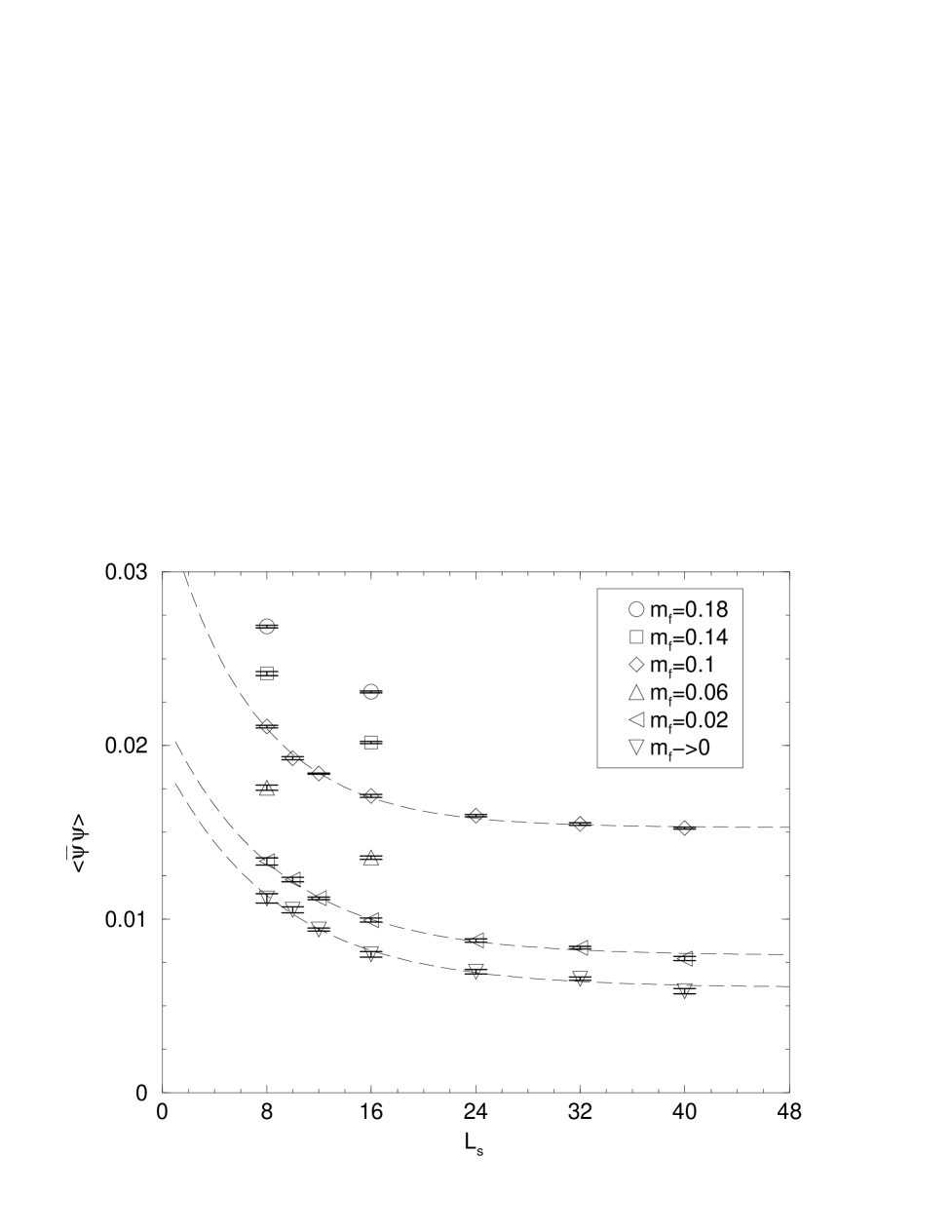
FIG. 9.: Full QCD values for $\langle\bar{\psi}\psi\rangle$ for $m_{0}=1.90$ and $\beta=5.2$ plotted versus $L_{s}$ for different values of $m_{f}$. The curves are fits of the form $c_{0}+c_{1}\exp(-\alpha L_{s})$.

FIG. 10.: Full QCD values for $\langle\bar{\psi}\psi\rangle$ for $m_{0}=1.90$ and $\beta=5.45$ versus $m_{f}$. The circles are for $L_{s}=8$, the squares for 16.

FIG. 11.: Full QCD values for $\langle\bar{\psi}\psi\rangle$ for $m_{0}=1.90$ and $\beta=5.45$ plotted versus $L_{s}$ for different values of $m_{f}$. The curves are fits of the form $c_{0}+c_{1}\exp(-\alpha L_{s})$.

FIG. 12.: Full QCD results for the Wilson line for $m_{f}=0.1$ and $L_{s}=12$ for different values of $m_{0}$ and $\beta$ near the transition region.

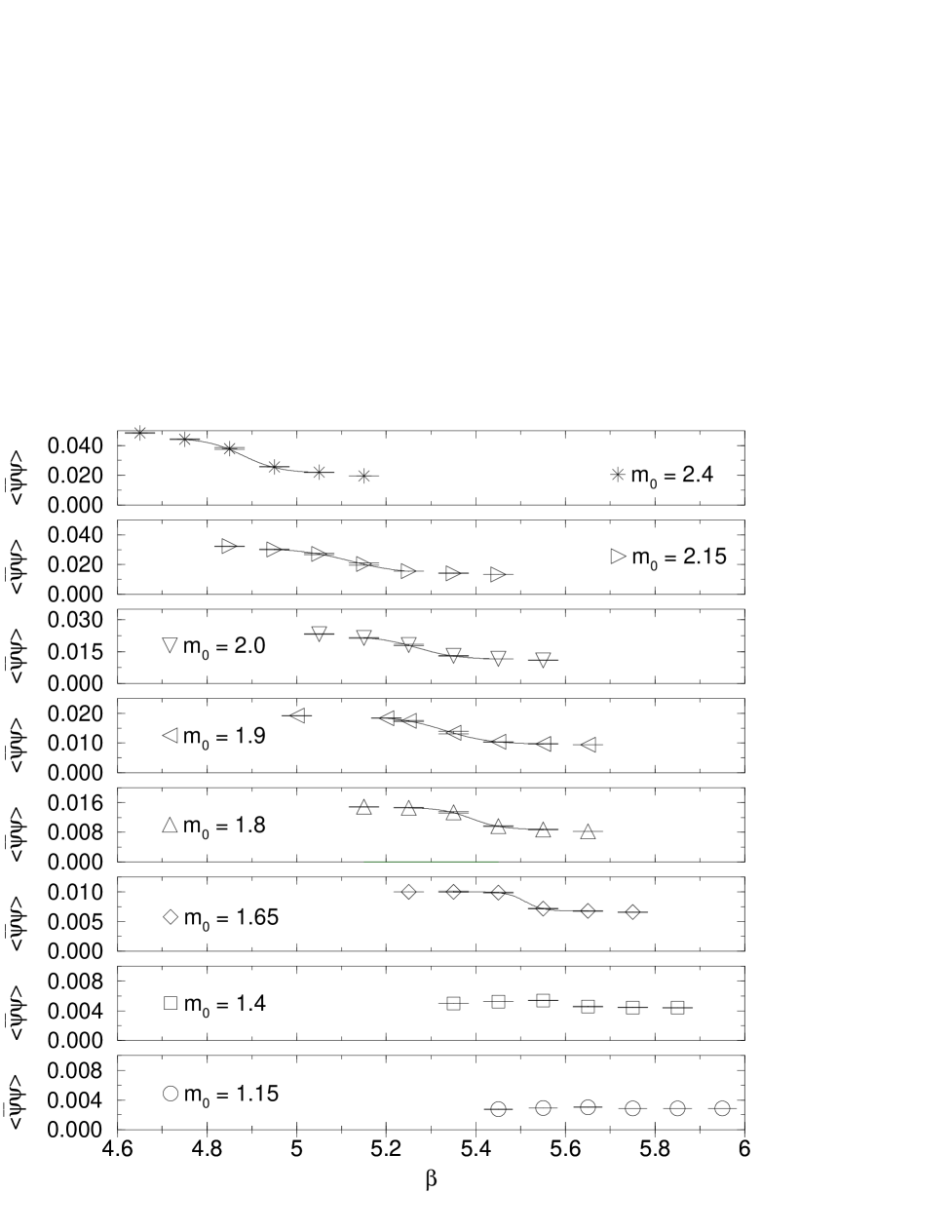
FIG. 13.: Full QCD results for $\langle\overline{\psi}\psi\rangle$ for $m_{f}=0.1$ and $L_{s}=12$ for different values of $m_{0}$ and $\beta$ near the transition region. Note that the vertical scale decreases by a factor of five as $m_{0}$ decreases from 2.4 to 1.15. This is needed to follow the large decrease in the scale of $\langle\overline{\psi}\psi\rangle$ which results from a combination of the decreasing lattice spacing that follows from increasing $\beta$ and the diminishing overlap of the light fermion states with the walls.

FIG. 14.: The critical value of $\beta$ as a function of $m_{0}$. The line is the value for a $24^{3}\times 4$ lattice.

FIG. 15.: The chiral condensate, $\langle\bar{\psi}\psi\rangle$, the pion susceptibility, $\chi_{\pi}$ and $\Delta J_{5}$ versus $L_{s}$ for $\beta=5.2$, $m_{0}=1.9$ and $m_{f}=0.02$.

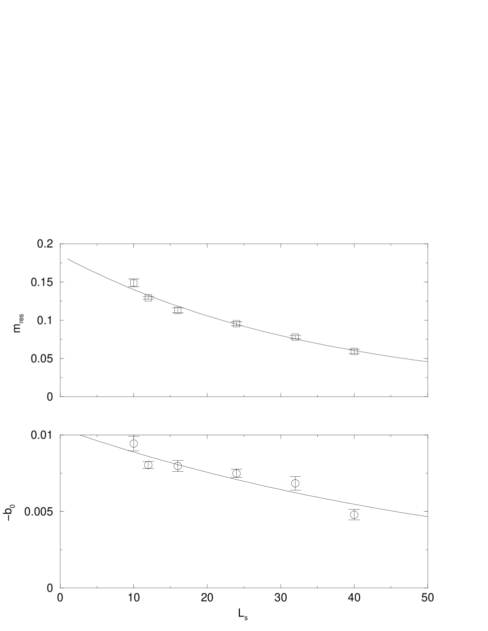
FIG. 16.: $m^{(\rm GMOR)}_{\rm res}$ and $-b_{0}$ versus $L_{s}$. The curves are fits to the form $c_{0}+c_{1}\exp(-\alpha L_{s})$.

$m_{f}$	$L_{s}$	traj. len.	# traj.	acc.	$\left\langle e^{-\Delta H}\right\rangle$	$\langle{\rm plaq}\rangle$	$\left\langle\left|W\right|\right\rangle$	$\left\langle\overline{\psi}\psi\right\rangle$
0.02	8	$\frac{1}{64}\times 32$	400-800	0.89	0.98(1)	0.456(2)	0.061(2)	0.0133(2)
	10	$\frac{1}{64}\times 32$	200-2000	0.86	0.995(8)	0.4460(9)	0.048(2)	0.0124(1)
	12	$\frac{1}{64}\times 32$	200-2000	0.84	1.01(1)	0.4428(6)	0.048(2)	0.01123(7)
	16	$\frac{1}{64}\times 32$	550-2000	0.75	0.98(2)	0.4388(9)	0.049(2)	0.00987(9)
	24	$\frac{1}{100}\times 50$	350-2000	0.73	0.95(2)	0.4359(7)	0.047(3)	0.0088(1)
	32	$\frac{1}{100}\times 50$	300-2000	0.72	1.03(2)	0.4317(7)	0.045(2)	0.00835(7)
	40	$\frac{1}{128}\times 64$	300-1350	0.73	1.02(3)	0.4342(6)	0.044(2)	0.00772(8)
0.06	8	$\frac{1}{50}\times 25$	200-950	0.83	0.98(1)	0.450(1)	0.046(3)	0.0176(2)
	16	$\frac{1}{64}\times 32$	200-820	0.84	0.99(2)	0.4361(8)	0.045(3)	0.0135(1)
0.1	8	$\frac{1}{40}\times 20$	300-800	0.57	0.89(5)	0.4437(8)	0.040(3)	0.02109(7)
	10	$\frac{1}{50}\times 25$	200-800	0.83	1.00(3)	0.4405(6)	0.036(2)	0.01927(9)
	12	$\frac{1}{40}\times 20$	400-800	0.43	1.2(3)	0.437(1)	0.032(2)	0.01838(4)
	16	$\frac{1}{64}\times 32$	200-800	0.80	0.98(2)	0.435(2)	0.035(2)	0.01709(9)
	24	$\frac{1}{64}\times 32$	200-800	0.72	0.94(2)	0.433(1)	0.033(2)	0.01596(7)
	32	$\frac{1}{100}\times 50$	200-800	0.82	0.99(2)	0.4305(5)	0.037(2)	0.01547(7)
	40	$\frac{1}{100}\times 50$	200-800	0.78	1.00(5)	0.432(1)	0.035(2)	0.01524(5)
0.14	8	$\frac{1}{40}\times 20$	200-860	0.63	1.03(6)	0.4433(7)	0.033(5)	0.0241(1)
	16	$\frac{1}{64}\times 32$	200-800	0.85	1.03(2)	0.433(1)	0.030(1)	0.02017(6)
0.18	8	$\frac{1}{40}\times 20$	200-1200	0.70	1.02(3)	0.4410(7)	0.030(1)	0.02686(7)
	16	$\frac{1}{64}\times 32$	200-800	0.84	0.98(2)	0.432(1)	0.033(1)	0.02309(5)

TABLE I.: Data for an $8^{3}\times 4$ lattice with $\beta=5.2$, $m_{0}=1.9$

$m_{f}$	$L_{s}$	traj. len.	# traj.	acc.	$\left\langle e^{-\Delta H}\right\rangle$	$\langle{\rm plaq}\rangle$	$\left\langle\left|W\right|\right\rangle$	$\left\langle\overline{\psi}\psi\right\rangle$
0.02	8	$\frac{1}{64}\times 32$	200-800	0.91	1.005(7)	0.5376(7)	0.226(4)	0.00415(6)
	10	$\frac{1}{64}\times 32$	200-1000	0.91	0.992(8)	0.5328(6)	0.207(4)	0.00319(5)
	12	$\frac{1}{64}\times 32$	200-800	0.95	1.009(9)	0.5300(4)	0.202(5)	0.00270(3)
	16	$\frac{1}{64}\times 32$	200-800	0.90	1.02(1)	0.5266(8)	0.199(4)	0.00237(6)
	24	$\frac{1}{64}\times 32$	400-1200	0.86	0.98(2)	0.5257(7)	0.187(3)	0.00216(6)
	32	$\frac{1}{100}\times 50$	400-800	0.94	1.00(2)	0.524(2)	0.180(5)	0.00209(5)
0.06	8	$\frac{1}{50}\times 25$	200-1000	0.86	0.99(3)	0.536(1)	0.217(3)	0.0080(1)
	10	$\frac{1}{64}\times 32$	200-1000	0.92	0.994(7)	0.5313(6)	0.203(4)	0.00704(5)
	12	$\frac{1}{64}\times 32$	200-1000	0.89	1.013(8)	0.5286(8)	0.195(4)	0.00666(5)
	16	$\frac{1}{64}\times 32$	400-800	0.76	1.02(4)	0.525(2)	0.192(4)	0.00637(7)
	24	$\frac{1}{64}\times 32$	300-1000	0.84	1.00(1)	0.521(2)	0.174(6)	0.00617(9)
	32	$\frac{1}{64}\times 32$	500-1000	0.80	1.00(2)	0.525(2)	0.189(3)	0.00592(4)
0.1	8	$\frac{1}{50}\times 25$	300-800	0.83	0.98(2)	0.5336(6)	0.211(4)	0.01174(4)
	10	$\frac{1}{50}\times 25$	300-990	0.88	0.99(1)	0.5310(9)	0.200(2)	0.01075(5)
	12	$\frac{1}{50}\times 25$	600-1200	0.74	1.01(4)	0.528(1)	0.197(4)	0.01838(4)
	16	$\frac{1}{64}\times 32$	400-800	0.79	1.01(3)	0.523(1)	0.170(5)	0.0103(1)
	24	$\frac{1}{64}\times 32$	400-2000	0.86	0.991(8)	0.512(1)	0.170(8)	0.0102(1)
	32	$\frac{1}{64}\times 32$	300-1000	0.81	0.98(2)	0.519(1)	0.159(5)	0.01011(9)
0.14	8	$\frac{1}{50}\times 25$	200-800	0.83	1.01(1)	0.533(1)	0.210(3)	0.01531(9)
	16	$\frac{1}{64}\times 32$	600-1200	0.76	0.98(2)	0.520(1)	0.159(9)	0.0143(1)
0.18	8	$\frac{1}{50}\times 25$	400-800	0.81	1.03(2)	0.5314(6)	0.202(4)	0.01884(5)
	16	$\frac{1}{64}\times 32$	600-1200	0.78	0.94(2)	0.515(1)	0.141(8)	0.0182(2)

TABLE II.: Data for an $8^{3}\times 4$ lattice with $\beta=5.45$, $m_{0}=1.9$

HMC traj. len: $\frac{1}{50}\times 25$,   CG stop cond: $10^{-6}$ $\beta$ start # traj acc. $\left\langle e^{-\Delta H}\right\rangle$ $\langle{\rm plaq}\rangle$ $\left\langle\left|W\right|\right\rangle$ $\left\langle\overline{\psi}\psi\right\rangle$ 5.45 O 100-800 0.87 0.99(1) 0.470(1) 0.0168(6) 0.00276(1) 5.55 O 200-800 0.87 0.98(1) 0.4933(6) 0.023(1) 0.002916(6) 5.65 O 300-800 0.87 1.00(2) 0.5218(9) 0.054(6) 0.00305(2) 5.75 D 300-800 0.86 0.986(9) 0.5571(7) 0.196(7) 0.002875(7) 5.85 D 300-800 0.85 1.00(1) 0.5719(7) 0.234(3) 0.002881(3) 5.95 D 200-800 0.87 0.99(1) 0.5857(5) 0.262(2) 0.002898(3)

TABLE III.: Data for an $8^{3}\times 4$ lattice with $m_{0}=1.15$, $L_{s}=12$, and $m_{f}=0.1$.

HMC traj. len: $\frac{1}{50}\times 25$,   CG stop cond: $10^{-6}$
$\beta$ start # traj acc. $\left\langle e^{-\Delta H}\right\rangle$ $\langle{\rm plaq}\rangle$ $\left\langle\left|W\right|\right\rangle$ $\left\langle\overline{\psi}\psi\right\rangle$ 5.35 O 100-800 0.87 1.01(1) 0.4435(7) 0.0189(8) 0.00497(1) 5.45 O 100-800 0.86 0.99(1) 0.4630(7) 0.0215(8) 0.00522(1) 5.55 O 300-800 0.86 1.00(1) 0.487(1) 0.032(3) 0.00539(3) 5.65 D 400-800 0.86 1.00(2) 0.540(2) 0.180(6) 0.00457(4) 5.75 D 300-800 0.85 0.99(1) 0.5598(8) 0.224(3) 0.00445(1) 5.85 D 200-800 0.89 1.011(8) 0.5744(3) 0.254(3) 0.004409(5)

TABLE IV.: Data for an $8^{3}\times 4$ lattice with $m_{0}=1.4$, $L_{s}=12$, and $m_{f}=0.1$.

HMC traj. len: $\frac{1}{50}\times 25$,   CG stop cond: $10^{-6}$ $\beta$ start # traj acc. $\left\langle e^{-\Delta H}\right\rangle$ $\langle{\rm plaq}\rangle$ $\left\langle\left|W\right|\right\rangle$ $\left\langle\overline{\psi}\psi\right\rangle$ 5.25 O 200-800 0.82 0.97(2) 0.4289(5) 0.027(2) 0.01000(2) 5.35 O 400-800 0.68 0.98(4) 0.451(3) 0.035(4) 0.01000(9) 5.45 D 400-800 0.74 1.09(5) 0.4769(8) 0.049(7) 0.00985(7) 5.55 D 600-1200 0.80 1.00(3) 0.531(1) 0.175(7) 0.00718(7) 5.65 D 400-800 0.79 0.96(2) 0.5507(9) 0.216(4) 0.00677(2) 5.75 D 200-800 0.88 0.989(7) 0.5663(4) 0.243(3) 0.00658(1)

TABLE V.: Data for an $8^{3}\times 4$ lattice with $m_{0}=1.65$, $L_{s}=12$, and $m_{f}=0.1$.

HMC traj. len: $\frac{1}{50}\times 25$,   CG stop cond: $10^{-6}$ $\beta$ start # traj acc. $\left\langle e^{-\Delta H}\right\rangle$ $\langle{\rm plaq}\rangle$ $\left\langle\left|W\right|\right\rangle$ $\left\langle\overline{\psi}\psi\right\rangle$ 5.15 O 200-800 0.83 1.02(2) 0.4191(8) 0.029(1) 0.01485(5) 5.25 O 400-800 0.66 0.97(5) 0.4381(6) 0.038(2) 0.01458(5) 5.35 O 400-800 0.63 0.97(5) 0.471(2) 0.052(3) 0.0134(2) 5.45 O 400-800 0.76 1.01(3) 0.515(2) 0.161(4) 0.0097(1) 5.55 D 400-800 0.79 1.05(5) 0.540(1) 0.200(9) 0.0088(1) 5.65 D 200-800 0.89 1.01(2) 0.5570(5) 0.242(4) 0.00828(2)

TABLE VI.: Data for an $8^{3}\times 4$ lattice with $m_{0}=1.8$, $L_{s}=12$, and $m_{f}=0.1$.

CG stop cond: $10^{-6}$ $\beta$ start traj. len. # traj acc. $\left\langle e^{-\Delta H}\right\rangle$ $\langle{\rm plaq}\rangle$ $\left\langle\left|W\right|\right\rangle$ $\left\langle\overline{\psi}\psi\right\rangle$ 5.0 O $\frac{1}{40}\times 20$ 200-800 0.37 0.8(1) 0.4002(8) 0.032(2) 0.01919(5) 5.2 O $\frac{1}{40}\times 20$ 400-800 0.43 1.2(3) 0.437(1) 0.032(2) 0.01838(4) 5.25 O $\frac{1}{50}\times 25$ 400-800 0.65 1.10(9) 0.452(1) 0.049(6) 0.0174(2) 5.35 D $\frac{1}{50}\times 25$ 600-1200 0.69 0.95(5) 0.493(2) 0.107(9) 0.0135(4) 5.45 D $\frac{1}{50}\times 25$ 600-1200 0.74 1.01(4) 0.528(1) 0.197(4) 0.01039(7) 5.55 D $\frac{1}{50}\times 25$ 400-830 0.82 1.00(1) 0.5463(5) 0.227(6) 0.00974(4) 5.65 D $\frac{1}{50}\times 25$ 400-800 0.88 1.03(1) 0.5613(8) 0.248(5) 0.00943(4)

TABLE VII.: Data for an $8^{3}\times 4$ lattice with $m_{0}=1.9$, $L_{s}=12$, and $m_{f}=0.1$.

HMC traj. len: $\frac{1}{50}\times 25$,   CG stop cond: $10^{-6}$ $\beta$ start # traj acc. $\left\langle e^{-\Delta H}\right\rangle$ $\langle{\rm plaq}\rangle$ $\left\langle\left|W\right|\right\rangle$ $\left\langle\overline{\psi}\psi\right\rangle$ 5.05 O 200-800 0.77 0.99(3) 0.4192(8) 0.035(1) 0.02324(8) 5.15 O 200-800 0.75 0.98(3) 0.442(1) 0.042(3) 0.0215(2) 5.25 O 200-1200 0.79 1.03(1) 0.474(1) 0.080(7) 0.0181(3) 5.35 D 200-800 0.83 1.00(2) 0.5130(7) 0.173(6) 0.0130(2) 5.45 D 200-800 0.87 1.02(2) 0.5349(5) 0.203(3) 0.01157(4) 5.55 D 200-800 0.85 1.01(1) 0.5503(4) 0.235(3) 0.01099(2)

TABLE VIII.: Data for an $8^{3}\times 4$ lattice with $m_{0}=2.0$, $L_{s}=12$, and $m_{f}=0.1$.

HMC traj. len: $\frac{1}{50}\times 25$,   CG stop cond: $10^{-6}$ $\beta$ start # traj acc. $\left\langle e^{-\Delta H}\right\rangle$ $\langle{\rm plaq}\rangle$ $\left\langle\left|W\right|\right\rangle$ $\left\langle\overline{\psi}\psi\right\rangle$ 4.85 O 200-800 0.69 0.95(3) 0.4004(8) 0.034(2) 0.0323(2) 4.95 O 200-800 0.72 0.97(3) 0.419(2) 0.040(2) 0.0302(3) 5.05 O 200-800 0.48 0.92(4) 0.443(2) 0.052(3) 0.0272(5) 5.15 O 200-1200 0.62 1.01(3) 0.480(3) 0.12(1) 0.0203(7) 5.25 O 400-800 0.70 0.97(5) 0.5105(4) 0.185(2) 0.01559(8) 5.35 D 400-800 0.69 1.01(4) 0.529(1) 0.216(6) 0.0141(1) 5.45 D 400-800 0.71 1.00(3) 0.5453(7) 0.230(4) 0.01330(5)

TABLE IX.: Data for an $8^{3}\times 4$ lattice with $m_{0}=2.15$, $L_{s}=12$, and $m_{f}=0.1$.

HMC traj. len: $\frac{1}{50}\times 25$,   CG stop cond: $10^{-6}$ $\beta$ start # traj acc. $\left\langle e^{-\Delta H}\right\rangle$ $\langle{\rm plaq}\rangle$ $\left\langle\left|W\right|\right\rangle$ $\left\langle\overline{\psi}\psi\right\rangle$ 4.65 O 100-800 0.63 1.02(5) 0.3953(6) 0.046(3) 0.0484(3) 4.75 O 200-800 0.68 0.99(5) 0.4156(9) 0.054(3) 0.0442(3) 4.85 O 300-800 0.70 0.94(4) 0.439(2) 0.069(5) 0.0380(6) 4.95 O 200-800 0.77 1.02(4) 0.4779(6) 0.155(4) 0.0257(2) 5.05 D 200-800 0.80 1.01(2) 0.4987(9) 0.190(2) 0.0220(2) 5.15 D 200-800 0.84 1.01(3) 0.5170(5) 0.221(3) 0.01962(7)

TABLE X.: Data for an $8^{3}\times 4$ lattice with $m_{0}=2.4$, $L_{s}=12$, and $m_{f}=0.1$.

$L_{s}$	$m_{\rm res}$	$-b_{0}$	$\chi^{2}/{\rm dof}$
10	0.149(5)	0.0094(5)	0.8(4)
12	0.129(2)	0.0080(2)	1.6(4)
16	0.113(3)	0.0080(4)	1.1(5)
24	0.095(2)	0.0075(3)	1.5(7)
32	0.078(2)	0.0068(5)	0.7(4)
40	0.059(3)	0.0048(3)	1.7(9)

TABLE XI.: Values for $m^{(\rm GMOR)}_{\rm res}$ and $-b_{0}$ versus $L_{s}$ from fits to valence quark data with the dynamical quark mass fixed at $m_{f}=0.02$.

REFERENCES

- [1] S. Bass et al. (1999), eprint nucl-th/9907090.
- [2] F. Karsch (1999), eprint hep-lat/9909006.
- [3] L. Kluberg, Nucl. Phys. A 661, 300c (1999).
- [4] R. Stock (1999), eprint hep-ph/9911408.
- [5] K. G. Wilson New Phenomena In Subnuclear Physics. Part A. Proceedings of the First Half of the 1975 International School of Subnuclear Physics, Erice, Sicily, July 11 - August 1, 1975, ed. A. Zichichi, Plenum Press, New York, 1977, p. 69, CLNS-321.
- [6] H. B. Nielsen and M. Ninomiya, Phys. Lett. B105, 219 (1981).
- [7] J. Kogut and L. Susskind, Phys. Rev. D11, 395 (1975).
- [8] T. Banks, L. Susskind, and J. Kogut, Phys. Rev. D13, 1043 (1976).
- [9] L. Susskind, Phys. Rev. D16, 3031 (1977).
- [10] R. D. Pisarski and F. Wilczek, Phys. Rev. D29, 338 (1984).
- [11] D. B. Kaplan, Phys. Lett. B288, 342 (1992), eprint hep-lat/9206013.
- [12] D. B. Kaplan, Nucl. Phys. Proc. Suppl. 30, 597 (1993).
- [13] Y. Shamir, Nucl. Phys. B406, 90 (1993), eprint hep-lat/9303005.
- [14] P. Vranas et al., Nucl. Phys. Proc. Suppl. 73, 456 (1999), eprint hep-lat/9809159.
- [15] P. Chen et al. (1998), eprint hep-lat/9812011.
- [16] P. Vranas (1999), eprint hep-lat/9903024.
- [17] D. Chen et al., Nucl. Phys. Proc. Suppl. 73, 898 (1999), eprint hep-lat/9810004.
- [18] P. Chen et al. In preparation.
- [19] P. Vranas, Nucl. Phys. Proc. Suppl. 53, 278 (1997), eprint hep-lat/9608078.
- [20] P. M. Vranas, Phys. Rev. D57, 1415 (1998), eprint hep-lat/9705023.
- [21] P. Chen et al., Phys. Rev. D59, 054508 (1999), eprint hep-lat/9807029.
- [22] R. Narayanan, Nucl. Phys. Proc. Suppl. 34, 95 (1994), eprint hep-lat/9311014.
- [23] M. Creutz, Nucl. Phys. Proc. Suppl. 42, 56 (1995), eprint hep-lat/9411033.
- [24] Y. Shamir, Nucl. Phys. Proc. Suppl. 47, 212 (1996), eprint hep-lat/9509023.
- [25] T. Blum, Nucl. Phys. Proc. Suppl. 73, 167 (1999), eprint hep-lat/9810017.
- [26] T. Blum and A. Soni, Phys. Rev. Lett. 79, 3595 (1997), eprint hep-lat/9706023.
- [27] T. Blum and A. Soni, Phys. Rev. D56, 174 (1997), eprint hep-lat/9611030.
- [28] R. Mawhinney et al., Nucl. Phys. Proc. Suppl. 73, 204 (1999), eprint hep-lat/9811026.
- [29] G. T. Fleming et al., Nucl. Phys. Proc. Suppl. 73, 207 (1999), eprint hep-lat/9811013.
- [30] A. L. Kaehler et al., Nucl. Phys. Proc. Suppl. 73, 405 (1999).
- [31] R. G. Edwards, U. M. Heller, and R. Narayanan, Nucl. Phys. B535, 403 (1998), eprint hep-lat/9802016.
- [32] G. T. Fleming (1999), eprint hep-lat/9909140.
- [33] L. Wu (RIKEN-BNL-CU) (1999), eprint hep-lat/9909117.
- [34] A. A. Khan et al. (CP-PACS) (1999), eprint hep-lat/9909049.
- [35] R. G. Edwards, U. M. Heller, and R. Narayanan, Phys. Rev. D60, 034502 (1999), eprint hep-lat/9901015.
- [36] S. Aoki, T. Izubuchi, Y. Kuramashi, and Y. Taniguchi (1999), eprint hep-lat/9909154.
- [37] S. Aoki, T. Izubuchi, Y. Kuramashi, and Y. Taniguchi (2000), eprint hep-lat/0004003.
- [38] P. Vranas, I. Tziligakis, and J. Kogut (1999), eprint hep-lat/9905018.
- [39] H. Neuberger, Phys. Rev. D57, 5417 (1998), eprint hep-lat/9710089.
- [40] H. Neuberger, Phys. Lett. B417, 141 (1998), eprint hep-lat/9707022.
- [41] H. Neuberger, Phys. Rev. Lett. 81, 4060 (1998), eprint hep-lat/9806025.
- [42] R. G. Edwards, U. M. Heller, and R. Narayanan, Phys. Rev. D59, 094510 (1999), eprint hep-lat/9811030.
- [43] C. Liu, Nucl. Phys. B554, 313 (1999), eprint hep-lat/9811008.
- [44] R. G. Edwards and U. M. Heller (2000), eprint hep-lat/0005002.
- [45] R. Narayanan and H. Neuberger (2000), eprint hep-lat/0005004.
- [46] S. Gottlieb, W. Liu, D. Toussaint, R. L. Renken, and R. L. Sugar, Phys. Rev. D35, 2531 (1987).
- [47] V. Furman and Y. Shamir, Nucl. Phys. B439, 54 (1995), eprint hep-lat/9405004.
- [48] R. Narayanan and H. Neuberger, Phys. Lett. B302, 62 (1993), eprint hep-lat/9212019.
- [49] R. Narayanan and H. Neuberger, Phys. Rev. Lett. 71, 3251 (1993), eprint hep-lat/9308011.
- [50] R. Narayanan and H. Neuberger, Nucl. Phys. B412, 574 (1994), eprint hep-lat/9307006.
- [51] R. Narayanan and H. Neuberger, Nucl. Phys. B443, 305 (1995), eprint hep-th/9411108.
- [52] T. A. DeGrand, Comput. Phys. Commun. 52, 161 (1988).
- [53] S. Aoki and Y. Taniguchi, Phys. Rev. D59, 054510 (1999), eprint hep-lat/9711004.
- [54] Y. Kikukawa, H. Neuberger, and A. Yamada, Nucl. Phys. B526, 572 (1998), eprint hep-lat/9712022.
- [55] P. Hernandez, K. Jansen, and M. Luscher, Nucl. Phys. B552, 363 (1999), eprint hep-lat/9808010.
- [56] H. Neuberger, Phys. Rev. D61, 085015 (2000), eprint hep-lat/9911004.
- [57] R. Narayanan and P. Vranas, Nucl. Phys. B506, 373 (1997), eprint hep-lat/9702005.
- [58] A. Vaccarino, Nucl. Phys. Proc. Suppl. 20, 263 (1991).
- [59] F. R. Brown, N. H. Christ, Y. F. Deng, M. S. Gao, and T. J. Woch, Phys. Rev. Lett. 61, 2058 (1988).