What are the Confining Field Configurations of Strong-Coupling Lattice Gauge Theory?

Abstract:

Starting from the strong-coupling SU(2) Wilson action in $D=3$ dimensions, we derive an effective, semi-local action on a lattice of spacing $L$ times the spacing of the original lattice. It is shown that beyond the adjoint color-screening distance, i.e. for $L\geq 5$, thin center vortices are stable saddlepoints of the corresponding effective action. Since the entropy of these stable objects exceeds their energy, center vortices percolate throughout the lattice, and confine color charge in half-integer representations of the SU(2) gauge group. This result contradicts the folklore that confinement in strong-coupling lattice gauge theory, for $D>2$ dimensions, is simply due to plaquette disorder, as is the case in $D=2$ dimensions. It also demonstrates explicitly how the emergence and stability of center vortices is related to the existence of color screening by gluon fields.

Quark confinement is commonly attributed to the influence of some special class of gauge field configurations, which dominate the QCD vacuum at large scales. Because of their high probability, these dominant configurations would most naturally correspond to the saddlepoints of an infrared effective action, derived at large scales by integrating over high-frequency modes. In strong-coupling lattice gauge theory there are methods available which enable us to compute the QCD spectrum and string tension analytically, and the same methods could also be applied to extract a long-range effective action. An interesting question, then, is what type of saddlepoint configurations are actually found at strong lattice couplings; it is likely that the answer would also shed some light on QCD in the continuum limit.

The classical Euclidean action of pure SU(N) gauge theory is stationary, or nearly so, at multi-instanton configurations. In quantized lattice gauge theory, however, we can imagine performing renormalization-group (RG) transformations so as to obtain an effective action at some scale $R$. For scales $R$ well below the confinement scale, the main effect of the RG transformations will simply be the running of the lattice coupling constant. At larger scales, however, so-called irrelevant operators can become important in the effective action. As a consequence, at these larger scales, the effective theory may have non-trivial saddlepoints which are something other than instantons.

There are good reasons to believe that at sufficiently large scales, these non-trivial saddlepoints are center vortices. On the theoretical side, we note that the asymptotic string tension between static color charges in SU(N) gauge theory depends only on the $N$-ality of the color charge representation. Although this fact is deduced rather trivially from the possibility of color-screening by gluon fields, it has some profound implications for the infrared structure of the QCD vacuum. Consider, for example, Wilson loops $W_{j}(C)$ in SU(2) gauge theory, where $j=0,\frac{1}{2},1,{3\over 2},...$ labels the group representation. Wilson loop expectation values can be viewed as a probe of vacuum fluctuations in the absence of external sources (think of evaluating a spacelike loop in the Hamiltonian formulation), and large Wilson loops are presumed to become “disordered,” i.e. have an area-law falloff, due to averaging over certain types of large-scale fluctuations which dominate the vacuum state. Whatever the nature of these confining fluctuations, they must have the highly non-trivial property of disordering only the $j=$ half-integer loops, but not the $j=$ integer loops. Center vortices are the only configurations we know of that have this property. Dual-superconductor models, in which all multiples of abelian electric charge (identified in an abelian-projection gauge) are confined by the dual Meissner effect, do not seem satisfactory. In these models, the potential between charged objects is roughly proportional to the electric charge. But this charge dependence cannot be correct, since gluons carrying two units of electric charge are available to screen multiply charged sources, and numerical simulations indicate that only odd multiples of the abelian charge (non-zero $N$-ality) are confined, while even multiples of abelian charge (zero $N$-ality) are screened [1]. Center vortices seem to be the natural way of accounting, in terms of dominant field configurations, for this very fundamental distinction between zero and non-zero $N$-ality, which is evident even in the abelian projection.

On the numerical side, there is now abundant evidence in favor of the vortex theory of confinement [2, 3, 4, 5, 6, 7, 8, 9, 10, 11, 12, 13], which we will not attempt to review here. The present situation can just be summarized as follows: There exists a method (known as “center projection”) for locating center vortices on thermalized lattices; the rationale undelying this method is explained in ref. [14]. By locating the vortices, their effects on gauge-invariant observables such as Wilson loops, Polyakov lines, topological charge, etc., can be studied in detail. The numerical evidence indicates that fluctuations in vortex linking number are the origin of the asymptotic string tension of Wilson loops. The free energy of a vortex, inserted into a finite lattice via twisted boundary conditions, has also been computed, and has been shown to fall off exponentially with the lattice size at just the rate predicted by the vortex theory [12, 13].

Vortices presumably have a finite thickness comparable to the adjoint string-breaking length, at about $1.25$ fm [15], where the crossover from Casimir scaling to $N$-ality confinement occurs (cf. the discussion in ref. [16]). Independent estimates of the vortex thickness are based on measurements of “vortex-limited” Wilson loops in ref. [4], and on the vortex free energy in finite volumes [12]. Both of these estimates put the vortex thickness at a little over one fermi. Beyond this scale, the presence of vortex sheets in the vacuum should be very evident. A reasonable conjecture is that if the appropriate effective action could be determined at this scale, it would be found to have stable saddlepoints corresponding to vortex configurations, which percolate through the lattice according to the usual energy-entropy arguments. Unfortunately, the calculation of long-range effective actions is very difficult even numerically, via Monte Carlo RG methods, and at such large scales the problem is quite intractable by perturbative (e.g. one-loop) methods.

We therefore turn our attention, in this article, to strong-coupling lattice gauge theory, where analytic methods can be brought to bear at arbitrarily large scales. In the strongly coupled theory in $D>2$ dimensions, we have a linear static potential for all color charge representations up to a screening scale of about four lattice spacings (for the SU(2) Wilson action). Beyond that scale, the string tension depends only on the $N$-ality of the representation, just as in the continuum theory. Thus, if our conjecture is correct, and if the $N$-ality dependence implies a vortex mechanism, the effective strong-coupling action at a scale beyond four lattice spacings should have saddlepoints which are stable center vortices.

There is, however, some folklore to the effect that confinement in strong coupling lattice gauge theory, in $D>2$ dimensions, is essentially the same as in $D=2$ dimensions, where the mechanism is simply plaquette disorder. If that were so, then vortices (or any other topological objects) are irrelevant at strong couplings in any dimension. This folklore is quite misleading, according to an argument presented in ref. [19], which we now review.

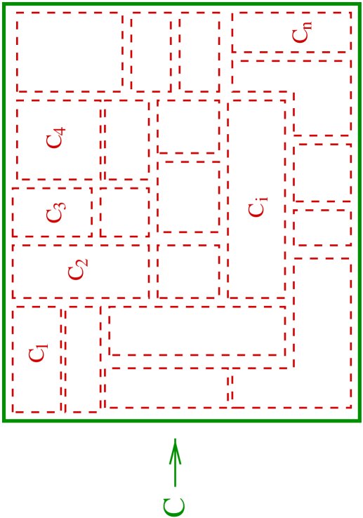
Figure 1: Decomposition of a large area bounded by planar loop $C$ into many sub-areas bounded by planar loops $\{C_{i}\}$

Consider SU(2) lattice gauge theory at strong-coupling, and denote by $U(C)$ the product of link variables around loop $C$. Let the minimal area of a planar loop be decomposed into a set of smaller areas, bounded by loops $\{C_{i}\}$, as shown in Fig. 1. The area-law of a Wilson loop is thought to be due to “magnetic disorder”, in which the gauge field strength fluctuates independently in sub-areas of the minimal surface of the loop. If this is so, then the holonomies $\{U(C_{i})\}$ should be (nearly) uncorrelated, for large areas and small $\beta$. The test for such independent fluctuation in the subareas $A(C_{i})$ is whether

$$<\prod_{i}F[U(C_{i})]>\stackrel{{\scriptstyle?}}{{=}}\prod_{i}<F[U(C_{i})]>$$ (1)

for any class function

$$F[g]=\sum_{j\neq 0}f_{j}\chi_{j}[g]$$ (2)

In fact, in $D=2$ dimensions, it is easy to show that this equality is satisfied exactly. However, for dimensions $D>2$, evaluating the left- and right-hand sides of (1) one finds for the exponential falloff on each side [19]

$$e^{-4\sigma{\cal P}(C)}\prod_{i}{1\over 3}f_{1}\gg\prod_{i}f_{1}e^{-4\sigma{\cal P}(C_{i})}$$ (3)

where the inequality holds for perimeters ${\cal P}(C)\ll\sum_{i}{\cal P}(C_{i})$. The conclusion is that the holonomies $U(C_{i})$ do not fluctuate independently, even at strong-coupling, for $D>2$.

If the loop holonomies in sub-areas of the loop are correlated, then where is the magnetic disorder required to give an area-law falloff for Wilson loops? The question is resolved by extracting a center element from the holonomies

$$z[U(C_{i})]=\mbox{signTr}[U(C_{i})]\in Z_{2}$$ (4)

and asking if these center elements fluctuate independently; i.e

$$<\prod_{i}z[U(C_{i})]>\stackrel{{\scriptstyle?}}{{=}}\prod_{i}<z[U(C_{i})]>$$ (5)

In fact, it is easy to show that they do:

$$e^{-\sigma A(C)}\prod_{i}{3\over 4\pi}=\prod_{i}{3\over 4\pi}e^{-\sigma A(C_{i})}$$ (6)

Thus, magnetic disorder is center disorder in $D>2$ dimensions, at least at strong couplings. Confining configurations must disorder the center elements $z$, but not the coset elements, of SU(2) holonomies $U(C_{i})$. Again, the only configurations known to have this property are center vortices.

We now return to our conjecture that vortices are stable saddlepoints of a long-range effective action. Actually, there are various ways of integrating out the smaller-scale fluctuations, to obtain an effective action at a larger scale. One simple approach is to superimpose, on a lattice of spacing $a$ with link variables denoted $U$, a lattice of spacing $La$ with links denoted $V$. An effective action for the lattice with the larger spacing can then be obtained from

$$\exp\Bigl{[}S_{eff}[V]\Bigr{]}=\int DU\prod_{l^{\prime}}\delta\Bigl{[}V^{\dagger}_{l^{\prime}}(UU..U)_{l^{\prime}}-I\Bigr{]}e^{S_{W}[U]}$$ (7)

where $(UU..U)_{l^{\prime}}$ is the product of $U$-link variables along the link $l^{\prime}$ of the V-lattice, and $S_{W}$ is the Wilson action. Obviously, all observables computed on the V-lattice with $S_{eff}$ will agree with the corresponding quantity computed on the U-lattice using $S_{W}$.

It is trivial to compute $S_{eff}$ in $D=2$ dimensions, and the result is

$$\exp\Bigl{[}S_{eff}[V]\Bigr{]}$$ (8)

$$\propto \prod_{P^{\prime}}\sum_{j}(2j+1)\Bigl{(}I_{2j+1}(\beta)\Bigr{)}^{L^{2}}\chi_{j}[V(P^{\prime})]$$

$$= \exp\left[\sum_{P^{\prime}}\log\left(1+\sum_{j=\frac{1}{2},1,{3\over 2}}(2j+1)\left({I_{2j+1}(\beta)\over I_{1}(\beta)}\right)^{L^{2}}\chi_{j}[V(P^{\prime})]\right)~{}+~{}\mbox{const.}\right]$$

$$\approx \exp\Bigl{[}2\left({\beta\over 4}\right)^{L^{2}}\sum_{P^{\prime}}\chi_{1/2}[V(P^{\prime})]~{}+~{}\mbox{const.}\Bigr{]}$$

where $V(P^{\prime})$ is the product of V-links around the plaquette $P^{\prime}$. One might imagine that the action (8) is also a good approximation in $D>2$ dimensions, at least at strong couplings, since this action gives the correct string tension for fundamental representation Wilson loops. But a quick calculation of higher representation loops shows that (8) cannot even be approximately correct for large $L$. A loop in the adjoint representation, for example, calculated on the U-lattice with the Wilson action, is easily seen to have an asymptotic perimeter law falloff

$$W_{adj}(C)\sim\exp[-\mu{\cal P}(C)]$$ (9)

where

$$\mu=-4\log\left({\beta\over 4}\right)$$ (10)

is the “gluelump” mass (gluon bound to a static adjoint color charge), and ${\cal P}(C)$ is the loop perimeter in units of the U-lattice spacing. However, carrying out the same calculation with the effective action (8), one finds instead (with ${\cal P}(C)$ again in U-lattice units) the erroneous result

$$\mu=-4L\log\left({\beta\over 4}\right)~{}~{}~{}~{}~{}~{}~{}~{}\mbox{(wrong)}$$ (11)

with an $L$-dependent gluelump mass. The mismatch is not resolved by including a few more contours in the effective action, so long as the coupling associated with each contour is of order $(\beta/4)^{A}$, where $A$ is the minimal area of the contour in U-lattice units.

Figure 2: Arrangement of U-plaquettes in a tube, around a rectangular contour $C$ on the V-lattice.

In fact, what happens in $D>2$ dimensions is that the effective action contains Wilson loops of all sizes in $j=$ integer representations, and these loops are only suppressed by perimeter-law coefficients. This is easily seen by bringing down a “tube” of plaquettes from $\exp(S_{W})$ in eq. (7), such that the tube borders a rectangular contour $C$ on the V-lattice, as shown in Fig. 2. Integrating over all U-links in the tube, except those which lie on contour $C$, will yield contributions to $S_{eff}$ such as

$$\exp\Bigl{[}S_{eff}[V]\Bigr{]} \supset \int DU_{l\in C}\prod_{l^{\prime}\in C}\delta\Bigl{[}V^{\dagger}_{l^{\prime}}(UU..U)_{l^{\prime}}-I\Bigr{]}\left({\beta\over 4}\right)^{4({\cal P}(C)-4)}\Bigl{(}\chi_{\frac{1}{2}}[U(C)]\Bigr{)}^{2}$$ (12)

$$\supset \left({\beta\over 4}\right)^{4({\cal P}(C)-4)}(\chi_{1}[V(C)]~{}+~{}\mbox{const.})$$

This shows that $S_{eff}[V]$ contains adjoint (and, in general, integer) representation loops with perimeter-falloff coefficients. Such non-local terms introduce non-local correlations among $SU(2)/Z_{2}$ coset elements in loop holonomies $\{U(C_{i})\}$. Truncating $S_{eff}[V]$ by removing these large loops will yield erroneous results for any Wilson loop in representation $j>\frac{1}{2}$.

Figure 3: The degrees of freedom in $\tilde{S}_{L}[V,\tilde{U}]$.

Our aim is to modify the prescription (7) for the effective action, in such a way that at least the leading contribution to any Wilson loop on the V-lattice is obtained from a local action. The strategy for doing this is to prevent the formation of closed tube diagrams, of the form shown in Fig. 2, bordering contours on the V-lattice. This can be accomplished by not integrating, in eq. (7), over the U-links in a cube of volume $2^{D}$ around each site on the V-lattice. U-links belonging to these 2-cubes will be denoted $\tilde{U}_{l}$. In order to ease the task of illustration, we will work in $D=3$ dimensions, although the extension to higher dimensions should be straightforward. We then have

$$Z = \int DV\int\prod_{l\in 2-cubes}d\tilde{U}_{l}~{}\exp\Bigl{[}\tilde{S}_{L}[V,\tilde{U}]\Bigr{]}$$ (13)

$$= \int DV\int\prod_{l\in 2-cubes}d\tilde{U}_{l}\left\{\int\prod_{l^{\prime\prime}\not\in 2-cubes}dU_{l^{\prime\prime}}\prod_{l^{\prime}}\delta\Bigl{[}V^{\dagger}_{l^{\prime}}(UU..U)_{l^{\prime}}-I\Bigr{]}e^{S_{W}[U]}\right\}$$

where the long-range action $\tilde{S}_{L}[V,\tilde{U}]$ depends on the $V$-link variables, and on the $\tilde{U}$-links in 2-cubes around sites of the V-lattice, as shown in Fig. 3.

Now introduce, in each 2-cube, a set of plaquette variables $\{h_{ij},g_{ij}\}$ which are Wilson lines beginning and ending at the center of the 2-cube, and running around one of the plaquettes in the cube. The $h_{ij}$ lines run around plaquettes on the faces of the 2-cube, and the $g_{ij}$ lines run around plaquettes on the interior of the 2-cubes. To fix notation: The orientation of the $g_{ij}$ lines is taken to be counterclockwise in either the $xy$-plane ($i=1$), the $yz$-plane ($i=2$), or the $zx$-plane ($i=3$). The second index ($j=1-4$) distinguishes between the four interior plaquettes in a given plane with the convention shown in Fig. 4, where $(x_{a},x_{b})=(xy),(yz),(zx)$. Each $h_{ij}$ line begins at the center of the 2-cube, runs to a center of one of the faces of the 2-cube, goes around one of the plaquettes on the face, and returns to the center of the 2-cube. The orientation around the $h$-plaquettes is defined by a right-hand rule: the thumb points in an outward direction normal to the 2-cube. The first index $i=1,2,3$ refers to a face of the 2-cube in the $xy$, $yz$, $zx$-planes, one lattice spacing away from the center of the 2-cube, in the negative $z,x,y$ directions, respectively. Index values $i=4,5,6$ refer to faces in the $xy$, $yz$, $zx$-planes one lattice spacing away from the center in the positive $z,x,y$ directions, respectively. These conventions are illustrated in Fig. 5.

Figure 4: Plaquette numbering convention.

Figure 5: Three plaquette variables on the 2-cube.

We then integrate over the $U$ links which do not belong to the 2-cubes. Keeping, for each type of contribution, only terms of leading order in $\beta$, the result is approximately

$$Z \approx \int DVD\tilde{U}~{}\exp\left[{\beta\over 2}\sum(\mbox{Tr}[h]+\mbox{Tr}[g])\right.$$ (14)

$$+2\left(\beta\over 4\right)^{4(L-2)}\sum_{l^{\prime}}f_{l^{\prime}}^{ijkl}\mbox{Tr}[h^{\dagger}_{ij}V_{l^{\prime}}h^{\dagger}_{kl}V^{\dagger}_{l^{\prime}}]$$

$$\left.+2\left({\beta\over 4}\right)^{L^{2}-4}\sum_{P^{\prime}}\mbox{Tr}[VgVgV^{\dagger}g^{\dagger}V^{\dagger}g^{\dagger}]\right]$$

Coefficients $f_{l^{\prime}}^{ijkl}=1$ if plaquette variables $h_{ij}$ and $h_{kl}$ on nearest-neighbor 2-cubes can be joined by a cylinder of plaquettes, bordering link $l^{\prime}$, of length $L-2$ U-lattice spacings. Otherwise, $f_{l^{\prime}}^{ijkl}=0$.

The next step is to change integration variables from links $\tilde{U}$ to plaquettes $g,h$. This change of variables on the lattice was worked out many years ago by Batrouni [20], and the result is simply to introduce a Bianchi constraint into the integration measure

$$Z \approx \int DVDhDg\prod_{2-cubes~{}K}~{}\prod_{c\in K}\delta[\mbox{Bianchi}(c(K))]$$ (15)

$$\exp\left[{\beta\over 2}\sum(\mbox{Tr}[h]+\mbox{Tr}[g])\right.$$

$$+2\left(\beta\over 4\right)^{4(L-2)}\sum_{l^{\prime}}f_{l^{\prime}}^{ijkl}\mbox{Tr}[h^{\dagger}_{ij}V_{l^{\prime}}h^{\dagger}_{kl}V^{\dagger}_{l^{\prime}}]$$

$$\left.+2\left({\beta\over 4}\right)^{L^{2}-4}\sum_{P^{\prime}}\mbox{Tr}[VgVgV^{\dagger}g^{\dagger}V^{\dagger}g^{\dagger}]\right]$$

Each 2-cube $K$ contains eight unit sub-cubes; the index $c$ in eq. (15) labels these subcubes. The $\delta$-function constraints force a certain product of three $g$ and three $h$ variables on each subcube to be the unit matrix. For example, the Bianchi constraint for the unit sub-cube containing $h_{11}$ is

$$\mbox{Bianchi}=h_{11}g_{23}h_{62}g^{\dagger}_{11}h_{53}g_{32}-I=0$$ (16)

Now expand the $\delta$-functions in group characters

$$\delta[\mbox{Bianchi}]=\sum_{j=0,\frac{1}{2},1,..}(2j+1)\chi_{j}[hghghg]$$ (17)

and integrate out the $g$-variables in eq. (15). Displaying only terms of low order in both $h$ and $\beta$, the result is

$$Z \approx \int DVDh\prod_{2-cubes~{}K}~{}\left\{1+2\left({\beta\over 4}\right)^{3}\sum_{c\in K}\chi_{\frac{1}{2}}[(hhh)_{c}]\right.$$ (18)

$$\left.+2\left({\beta\over 4}\right)^{4}\sum_{\stackrel{{\scriptstyle adjacent}}{{c_{1}c_{2}\in K}}}\chi_{\frac{1}{2}}[(hhh)_{c_{1}}(hhh)_{c_{2}}]+...\right\}$$

$$\times \exp\left[{\beta\over 2}\sum\mbox{Tr}[h]+2\left(\beta\over 4\right)^{4(L-2)}\sum_{l^{\prime}}f_{l^{\prime}}^{ijkl}\mbox{Tr}[h^{\dagger}_{ij}V_{l^{\prime}}h^{\dagger}_{kl}V^{\dagger}_{l^{\prime}}]\right.$$

$$\left.+2\left({\beta\over 4}\right)^{L^{2}}\sum_{P^{\prime}}\mbox{Tr}[VVV^{\dagger}V^{\dagger}]\right]$$

$$\approx \int DVDh~{}\exp\Bigl{[}S_{L}[V,h]\Bigr{]}$$

At this stage, the action $S_{L}[V,h]$ resembles an adjoint-Higgs Lagrangian, albeit of an unconventional form: There is an SU(2) gauge field $V_{\mu}$ coupled to 24 unitary matrix-valued “matter” fields $h_{ij}$ transforming in the adjoint representation. These matter fields, in turn, can be subdivided into gauge-singlet fields $h_{ij,0}$, and unit-modulus triplet fields $\vec{e}_{ij}$, where

$$h_{ij}=h_{ij,0}I+i\sqrt{1-h^{2}_{ij,0}}\vec{e}_{ij}\cdot\vec{\sigma}$$ (19)

and $\vec{e}\cdot\vec{e}=1$. The unimodular $\vec{e}_{ij}$ degrees of freedom play a role analogous to Higgs fields. We know from the Elitzur theorem that the expectation values of these fields must vanish in the absence of gauge fixing, and cannot be viewed as order parameters. Since the coupling of the $\vec{e}_{ij}$ matter fields to the $V_{\mu}$ gauge field is very weak at large $L$, as compared to the self-couplings of the $\vec{e}_{ij}$ fields to each other on the 2-cubes, their expectation values depend primarily on these self-couplings, and on the complete removal of gauge redundancy in the $e$-fields through the choice of a unitary gauge.

We fix to a maximal unitary gauge by first transforming one of the 24 unimodular “Higgs” fields $\vec{e}_{ij}$ on each 2-cube, denoted $\vec{e}_{A}$, to point in the (color) 3-direction, i.e.

$$e_{A1}=e_{A2}=0~{}~{},~{}~{}e_{A3}=1$$ (20)

This leaves a remnant U(1) symmetry, but (20) is not yet a maximal unitary gauge fixing. We then pick one other Higgs variable on each 2-cube, denoted $\vec{e}_{B}$, and use the remaining gauge freedom to fix

$$e_{B2}=0~{}~{},~{}~{}e_{B1}=\sin(\theta_{B})\geq 0$$ (21)

leaving a remnant $Z_{2}$ symmetry.

In the unitary gauge [20-21], the functional integral becomes

$$Z_{ug}=\int\prod_{n}dV(n)\prod_{ij}dh_{ij}(n)\Delta(h_{A},h_{B})\delta(e_{A1})\delta(e_{A2})\delta(e_{B2})\exp\Bigl{[}S_{L}[V,h]\Bigr{]}$$ (22)

where

$$\Delta^{-1}(h_{A},h_{B}) = \int d^{3}\alpha~{}\delta(e^{\alpha}_{A1})\delta(e^{\alpha}_{A2})\delta(e^{\alpha}_{B2})$$ (23)

$$= \int d^{3}\alpha~{}\delta(\epsilon_{1jk}\alpha_{j}\delta_{3k})\delta(\epsilon_{2jk}\alpha_{j}\delta_{3k})\delta(\epsilon_{2jk}\alpha_{j}(e_{B1}\delta_{1k}+e_{B3}\delta_{3k}))$$

$$= e^{-1}_{B1}$$

From the measure

$$\int dh=\int dh_{0}d^{3}e~{}\sqrt{1-h_{0}^{2}}\delta(e^{2}-1)$$ (24)

we find

$$\int dh_{A}dh_{B}~{}\Delta(h_{A},h_{B})\delta(e_{A1})\delta(e_{A2})\delta(e_{B2})=\int dh_{A0}dh_{B0}d\theta_{B}\sqrt{1-h_{A0}^{2}}\sqrt{1-h_{B0}^{2}}\sin\theta_{B}$$ (25)

Let us take, e.g., $h_{A}=h_{11},~{}h_{B}=h_{44}$. Then

$$Z_{ug} = \int\prod_{n}dV(n)\int dh_{11,0}dh_{44,0}d\theta_{44}\sqrt{1-h_{11,0}^{2}}\sqrt{1-h_{44,0}^{2}}\sin\theta_{44}$$ (26)

$$\prod_{ij\neq(11),(44)}dh_{ij}(n)\exp\Bigl{[}S_{L}[V,h]\Bigr{]}$$

The final step is to integrate over the remaining $h$ degrees of freedom in this maximal unitary gauge. Defining $h$-expectation values

$$\langle F[h]\rangle_{h}~{}=~{}$$ (27)

$${1\over{\cal Z}_{h}}\int dh_{11,0}dh_{44,0}d\theta_{44}\sqrt{1-h_{11,0}^{2}}\sqrt{1-h_{44,0}^{2}}\sin\theta_{44}\prod_{ij\neq(11),(44)}dh_{ij}(n)$$

$$\prod_{2-cubes~{}K}~{}\left\{1+2\left({\beta\over 4}\right)^{3}\sum_{c\in K}\chi_{\frac{1}{2}}[(hhh)_{c}]+2\left({\beta\over 4}\right)^{4}\sum_{\stackrel{{\scriptstyle adjacent}}{{c_{1}c_{2}\in K}}}\chi_{\frac{1}{2}}[(hhh)_{c_{1}}(hhh)_{c_{2}}]+...\right\}$$

$$\times\exp\left[{\beta\over 2}\sum\mbox{Tr}[h]\right]F[h]$$

and

$$S_{eff}[V,h] = 2\left(\beta\over 4\right)^{4(L-2)}\sum_{l^{\prime}}f_{l^{\prime}}^{ijkl}\mbox{Tr}[h^{\dagger}_{ij}V_{l^{\prime}}h^{\dagger}_{kl}V^{\dagger}_{l^{\prime}}]$$ (28)

$$+2\left({\beta\over 4}\right)^{L^{2}}\sum_{P^{\prime}}\mbox{Tr}[VVV^{\dagger}V^{\dagger}]$$

we have

$$Z_{ug} = {\cal Z}_{h}\int DV\left\langle\exp\Bigl{[}S_{eff}[V,h]\Bigr{]}\right\rangle_{h}$$ (29)

$$= {\cal Z}_{h}\int DV\exp\Bigl{[}S_{eff}[V]\Bigr{]}$$

where

$$S_{eff}[V]=S_{eff}[V,\langle h\rangle_{h}]+\mbox{higher-order contributions}$$ (30)

The higher-order contributions consist of next-nearest neighbor (and more distant) couplings between $\langle h\rangle_{h}$ terms on different 2-cubes, as well as closed loops in $j=1$ and higher representations. The large closed loops again introduce certain non-local correlations among the $SU(2)/Z_{2}$ elements of loop holonomies $\{U(C_{i})\}$. But $S_{eff}[V]$ also contains local one-link terms, which provide by far the largest contribution to the $Z_{2}$-invariant part of the action.

For the purpose of determining saddlepoint configurations of $S_{eff}[V]$ we may neglect the higher-order, non-local terms in the action, so that

$$S_{eff}[V] \approx S_{link}[V,\langle h\rangle_{h}]+S_{plaq}[V]$$ (31)

$$= 2\left({\beta\over 4}\right)^{4(L-2)}\sum_{l^{\prime}}f_{l^{\prime}}^{ijkl}\mbox{Tr}\Bigl{[}\langle h^{\dagger}_{ij}\rangle_{h}V_{l^{\prime}}\langle h^{\dagger}_{kl}\rangle_{h}V^{\dagger}_{l^{\prime}}\Bigr{]}$$

$$+2\left({\beta\over 4}\right)^{L^{2}}\sum_{P^{\prime}}\mbox{Tr}[VVV^{\dagger}V^{\dagger}]$$

and, for this particular gauge choice, we find

$$\begin{array}[]{lcl}\langle h_{11}\rangle_{h}={\beta\over 4}I+i{8\over 3\pi}\sigma_{3}&~{},{}&\langle h_{12}\rangle_{h}={\beta\over 4}I-i\left({\beta\over 4}\right)^{8}{8\over 3\pi}\sigma_{3}\cr\langle h_{13}\rangle_{h}={\beta\over 4}I-i\left({\beta\over 4}\right)^{8}{8\over 3\pi}\sigma_{3}&~{},{}&\langle h_{14}\rangle_{h}={\beta\over 4}I-i\left({\beta\over 4}\right)^{8}{2\over 3}\sigma_{1}\cr\langle h_{41}\rangle_{h}={\beta\over 4}I-i\left({\beta\over 4}\right)^{8}{8\over 3\pi}\sigma_{3}&~{},{}&\langle h_{42}\rangle_{h}={\beta\over 4}I-i\left({\beta\over 4}\right)^{8}{2\over 3}\sigma_{1}\cr\langle h_{43}\rangle_{h}={\beta\over 4}I-i\left({\beta\over 4}\right)^{8}{2\over 3}\sigma_{1}&~{},{}&\langle h_{44}\rangle_{h}={\beta\over 4}I+i{2\over 3}\sigma_{1}\cr\langle h_{21}\rangle_{h}={\beta\over 4}I-i\left({\beta\over 4}\right)^{8}{2\over 3}\sigma_{1}&~{},{}&\langle h_{22}\rangle_{h}={\beta\over 4}I-i\left({\beta\over 4}\right)^{4}{2\over 3}\sigma_{1}\cr\langle h_{23}\rangle_{h}={\beta\over 4}I-i\left({\beta\over 4}\right)^{8}{8\over 3\pi}\sigma_{3}&~{},{}&\langle h_{24}\rangle_{h}={\beta\over 4}I-i\left({\beta\over 4}\right)^{8}{2\over 3}\sigma_{1}\cr\langle h_{51}\rangle_{h}={\beta\over 4}I-i\left({\beta\over 4}\right)^{8}{8\over 3\pi}\sigma_{3}&~{},{}&\langle h_{52}\rangle_{h}={\beta\over 4}I-i\left({\beta\over 4}\right)^{8}{2\over 3}\sigma_{1}\cr\langle h_{53}\rangle_{h}={\beta\over 4}I-i\left({\beta\over 4}\right)^{4}{8\over 3\pi}\sigma_{3}&~{},{}&\langle h_{54}\rangle_{h}={\beta\over 4}I-i\left({\beta\over 4}\right)^{8}{8\over 3\pi}\sigma_{3}\cr\langle h_{31}\rangle_{h}={\beta\over 4}I-i\left({\beta\over 4}\right)^{8}{2\over 3}\sigma_{1}&~{},{}&\langle h_{32}\rangle_{h}={\beta\over 4}I-i\left({\beta\over 4}\right)^{4}{2\over 3}\sigma_{1}\cr\langle h_{33}\rangle_{h}={\beta\over 4}I-i\left({\beta\over 4}\right)^{8}{2\over 3}\sigma_{1}&~{},{}&\langle h_{34}\rangle_{h}={\beta\over 4}I-i\left({\beta\over 4}\right)^{8}{8\over 3\pi}\sigma_{3}\cr\langle h_{61}\rangle_{h}={\beta\over 4}I-i\left({\beta\over 4}\right)^{8}{8\over 3\pi}\sigma_{3}&~{},{}&\langle h_{62}\rangle_{h}={\beta\over 4}I-i\left({\beta\over 4}\right)^{8}{2\over 3}\sigma_{1}\cr\langle h_{63}\rangle_{h}={\beta\over 4}I-i\left({\beta\over 4}\right)^{4}{8\over 3\pi}\sigma_{3}&~{},{}&\langle h_{64}\rangle_{h}={\beta\over 4}I-i\left({\beta\over 4}\right)^{8}{8\over 3\pi}\sigma_{3}\end{array}$$ (32)

Inserting (32) into $S_{link}$ we have, to leading order in $\beta$,

$$S_{link}[V,\langle h\rangle_{h}]=2\left({\beta\over 4}\right)^{4(L-2)}\times\sum_{n}$$ (33)

$$\left\{\left({8\over 3\pi}\right)^{2}\left({\beta\over 4}\right)^{8}\mbox{Tr}[\sigma_{3}V_{z}(n)\sigma_{3}V^{\dagger}_{z}(n)]+\left({2\over 3}\right)^{2}\left({\beta\over 4}\right)^{8}\mbox{Tr}[\sigma_{1}V_{z}(n)\sigma_{1}V^{\dagger}_{z}(n)]\right.$$

$$-\left({8\over 3\pi}\right)^{2}\left({\beta\over 4}\right)^{12}\mbox{Tr}[\sigma_{3}V_{y}(n)\sigma_{3}V^{\dagger}_{y}(n)]-\left({2\over 3}\right)^{2}\left({\beta\over 4}\right)^{12}\mbox{Tr}[\sigma_{1}V_{y}(n)\sigma_{1}V^{\dagger}_{y}(n)]$$

$$-\left({8\over 3\pi}\right)^{2}\left({\beta\over 4}\right)^{12}\mbox{Tr}[\sigma_{3}V_{x}(n)\sigma_{3}V^{\dagger}_{x}(n)]-\left({2\over 3}\right)^{2}\left({\beta\over 4}\right)^{12}\mbox{Tr}[\sigma_{1}V_{x}(n)\sigma_{1}V^{\dagger}_{x}(n)]$$

$$+~{}\mbox{const.}\Bigr{\}}$$

Each term in $S_{link}$ is proportional to a component of a $V$-link variable in the adjoint representation, and is insensitive to the center degrees of freedom. The spatial asymmetry of $S_{link}$ in (33) is, of course, due to the particular unitary gauge choice.

We now look for saddlepoints of $S_{eff}$. It can be seen from inspection of (33) that $S_{link}$ is maximized by

$$V_{x}(n)=i\sigma_{2}Z_{x}(n)~{}~{},~{}~{}V_{y}(n)=i\sigma_{2}Z_{y}(n)~{}~{},~{}V_{z}(n)=Z_{z}(n)$$ (34)

where the $Z_{\mu}(n)=\pm I$ are center elements. The $S_{plaq}$ term is also maximized if the $Z_{\mu}$ link variables are gauge-equivalent to the identity under the remnant $Z_{2}$ gauge symmetry. With this choice the effective action $S_{eff}\approx S_{link}+S_{plaq}$ is maximized, and the configuration (34) is the ground state, gauge equivalent to the identity. The fact that this ground state is unique, up to a $Z_{2}$ gauge transformation, is again due to the maximal unitary gauge fixing.

Now consider the configuration

$$V_{y}(\vec{n}) = \left\{\begin{array}[]{rl}-i\sigma_{2}&n_{1}\geq 2,~{}n_{2}=1\cr+i\sigma_{2}&\mbox{otherwise}\end{array}\right.$$ (37)

$$V_{x}(\vec{n}) = i\sigma_{2}$$

$$V_{z}(\vec{n}) = I$$ (38)

This configuration is a center vortex, one lattice spacing thick, running in the $z$-direction. It is not hard to see that this configuration, like the trivial ground state, is also a saddlepoint of $S_{eff}$. In the first place, (38) is a global maximum of $S_{link}$, since the thin vortex configuration (38) differs from link variables in the ground state only by center elements, to which $S_{link}$ is insensitive. Secondly, this configuration is also a stationary point of the plaquette action $S_{plaq}$ [21]. This is because a plaquette at one of its extremal values $\frac{1}{2}\mbox{Tr}[VVV^{\dagger}V^{\dagger}]=\pm 1$ varies at most quadratically, and is therefore stationary, with respect to a small variation $\delta V$ of any link respecting the unitarity constraint $(V+\delta V)(V+\delta V)^{\dagger}=I$. All of the plaquettes formed from (38) are extremal. So the center vortex (38) is certainly a stationary configuration of $S_{eff}$, the remaining question is whether it is stable; i.e. whether the vortex is a local maximum of $S_{eff}$, in which case it is a stable saddlepoint.

The stability issue is settled by looking at the eigenvalues of

$${\delta^{2}S_{eff}\over\delta V_{\mu}(n_{1})\delta V_{\nu}(n_{2})}={\delta^{2}S_{link}\over\delta V_{\mu}(n_{1})\delta V_{\nu}(n_{2})}+{\delta^{2}S_{plaq}\over\delta V_{\mu}(n_{1})\delta V_{\nu}(n_{2})}$$ (39)

where, from the coefficients shown in eqs. (31) and (33), we see that

$${\delta^{2}S_{link}\over\delta V_{\mu}(n_{1})\delta V_{\nu}(n_{2})}\sim\left({\beta\over 4}\right)^{4(L-2)+12}~{}~{}~{},~{}~{}~{}{\delta^{2}S_{plaq}\over\delta V_{\mu}(n_{1})\delta V_{\nu}(n_{2})}\sim\left({\beta\over 4}\right)^{L^{2}}$$ (40)

The crucial observation is that for $\beta/4\ll 1$ and

$$4(L-2)+12<L^{2}$$ (41)

the contribution of $S_{plaq}$ to the stability matrix (and therefore to the eigenvalues of the stability matrix) is negligible compared to the contribution of $S_{link}$, which has only stable modes. Thus from the fact that the thin center vortex (38) is both a stationary point of $S_{eff}$, and a stable saddlepoint of $S_{link}$, we can conclude that the vortex is also a stable saddlepoint of the full effective action $S_{eff}$ when condition (41) is satisfied.

Condition (41) is satisfied for $L\geq 5$ lattice spacings. It is probably no coincidence that this is also where the adjoint string breaks in strong-coupling lattice gauge theory (as can be easily verified from looking at correlations of Polyakov lines in the adjoint representation). It has been known for a long time that, at intermediate distance scales and weak couplings, the static quark-antiquark potential is roughly (and maybe even accurately [22]) proportional to the quadratic Casimir of quark color representation. In ref. [23] this phenomenon was dubbed “Casimir scaling,” and the problems it poses for monopole and vortex theories was discussed. In ref. [16] we have argued that the problems with respect to the vortex theory can in principle be resolved by taking into account the finite thickness of the vortex, which should be comparable to the adjoint string-breaking length. A result of the analysis carried out above is that there are stable center vortices, one lattice spacing thick on the V-lattice, corresponding to $L\geq 5$ on the original U-lattice. This gives an estimate for the vortex thickness of $L=4$ lattice spacings in U-lattice units. This vortex thickness happens to be exactly the length where adjoint string-breaking occurs in the strong-coupling Wilson action, and is therefore consistent with the reasoning in ref. [16].

By inspection of $S_{eff}$, we see that the action of a center vortex configuration in D=3 dimensions (ignoring any further quantum corrections) is

$$8\left({\beta\over 4}\right)^{L^{2}}~{}\times~{}\mbox{vortex length}$$ (42)

on the V-lattice. On the other hand, the entropy of a linelike object (essentially the entropy of a random walk) is a constant of $O(1)$ times the line length. Thus, center vortices are stable saddlepoints of the long range effective action whose entropy per unit length greatly exceeds their action per unit length. These objects therefore percolate throughout the lattice volume, and confine color charge in any half-integer group representation.

This picture has been derived in a particular unitary gauge. A natural question is whether the saddlepoints of the effective action would be qualitatively different had we chosen to gauge-fix, instead of $\vec{e}_{11}$ and $\vec{e}_{44}$, some other plaquette variables (or combination of plaquette variables) on the 2-cubes. Although an analysis of all possible unitary gauge choices is beyond us at present, it is easy to see that center vortices must be stable saddlepoints in a very large class of gauges. We first note that, by definition, any maximal unitary gauge must completely determine the minimal action configuration of the $V_{\mu}$ fields, up to residual $Z_{2}$ gauge transformations. Then a sufficient condition for center vortex stability is simply that the classical ground state of $S_{eff}[V]$ has the form of a pure gauge $V_{\mu}(x)=g(x)g^{-1}(x+\hat{\mu})$, and that this is also a maximum of the center-invariant $S_{link}$ part of the effective action. In that case, the effective action must have stable thin vortex solutions at large $L$. This is because the stable fluctuation modes around a thin vortex, associated with the center-insensitive $S_{link}$ term, will overwhelm (at sufficiently large $L$) any unstable modes associated with $S_{plaq}$. The vortex action at a given $L$ will always have the value shown in eq. (42) above, so the entropy of the configuration will exceed the action at strong couplings.

Our findings for the strong-coupling theory do not, however, prove that vortices also dominate the vacuum at weaker couplings; the strong and weak coupling regimes are separated by a roughening phase transition, and this transition prevents a simple extrapolation from one regime to the other. The result is, nonetheless, significant for continuum physics in two ways: First, it supports the very general argument that if the asymptotic quark potential is sensitive only to $N$-ality, then the confining field configurations must be center vortices. Secondly, it provides an explicit illustration of how center vortices are stabilized, via color-screening (center-invariant) terms in the long-range effective action.

Although strong-coupling methods only apply at strong couplings, the general approach we have advocated here should extend, at least in principle, to weak-coupling lattice gauge theory. The central idea is that if we want to extract a local long-range effective action from the Wilson action, then it is necessary to include composite operators, transforming like adjoint matter fields, in the derivation. With this motivation we define gluelump operators

$$G_{M}[x;U]=\sum_{C_{x}}a_{M}(C_{x})\prod_{l\in C_{x}}U_{l}$$ (43)

which, coupled to a static adjoint source at site $x$, create gauge-invariant eigenstates of the appropriate transfer matrix. The $C_{x}$ are paths on the lattice beginning and ending at $x$. The index $M$ specifies the time (i.e. worldline) direction of the static source, and any other (e.g. spin) degeneracies. The transformation from a pure gauge theory on a fine lattice, to a theory of gauge fields $V_{\mu}$ coupled to gluelump fields $H_{M}$ on a coarse lattice, could then be accomplished as follows:

$$\exp\Bigl{[}S_{eff}[V,H]\Bigr{]}=\int DU\prod_{l^{\prime}}\delta\Bigl{(}V_{l^{\prime}}-Q_{l^{\prime}}[U]\Bigr{)}\prod_{M,x^{\prime}}\delta\Bigl{(}H_{M}(x^{\prime})-G_{M}[x^{\prime};U]\Bigr{)}e^{S_{W}[U]}$$ (44)

where $x^{\prime},l^{\prime}$ denote sites and links on the coarse lattice. The expression $Q_{l^{\prime}}[U]$ represents a suitable “fat link” function, i.e. a superposition of Wilson lines on the fine lattice which run between sites bounding link $l^{\prime}$ on the coarse lattice. The constraints imposed by the delta-functions can be softened by replacing delta-functions with exponentials, as in the “perfect action” approach [24]. The end result of this procedure will be an effective long-range action consisting of gauge fields coupled to a set of adjoint Higgs-like fields. Possibly this scheme can be implemented numerically at moderately weak couplings, along the lines of the Monte Carlo renormalization-group.

In the strong-coupling analysis carried out in this article, we have seen how color-screening, center-invariant “Higgs” terms predominate in the long-range effective action beyond the adjoint string-breaking scale, and stabilize center vortex configurations. The entropy of these configurations exceeds the cost in action, and vortex configurations percolate throughout the lattice. We think it likely that these important features are not specific to strong couplings, and also characterize the effective action of lattice QCD in the continuum limit.