A disorder analysis of the Ising model

Abstract

Lattice studies of monopole condensation in QCD are based on the construction of a disorder parameter, a creation operator of monopoles which is written in terms of the gauge fields. This procedure is expected to work for any system which presents duality. We check it on the Ising model in $2d$, which is exactly solvable. The output is an amusing exercise in statistical mechanics.

, ,

1 Introduction

Duality [1, 2] is a property of many systems in field theory and in statistical mechanics. Their common feature is that, when viewed as Euclidean field theories, they have spatial [$(d-1)$-dimensional] configurations carrying a conserved topological charge. The high temperature (strong coupling) phase is characterized by condensation of these topological structures. In a dual description these structures are described by local fields, and their v.e.v. acts as a dual order parameter, or disorder parameter.

In a few models the transformation to the dual is known analytically (the Ising model, the U(1) model with Villain action [3], the $3d$ XY model). In other theories duality is expected to be at work, but its presence has only been tested numerically [4, 5, 6, 7, 8, 9]. The idea is to guess the topological symmetries classifying the extended structures, construct a disorder parameter as the creation operator of a structure with non-trivial topology [10], and then measure it by numerical simulations [4, 5, 6, 7, 8, 9].

The approach [10, 4, 5, 6, 7, 8, 9] relies on symmetry, and is insensitive to the exact choice of the action, or to irrelevant terms, contrary to the explicit transformation to the dual, which is only possible for specific forms of the action (the Villain action in the XY model and in the U(1) model in $(3+1)d$).

A test of the construction is the determination of the critical indices at the phase transition by finite size scaling analysis. This has already been done for QCD [9], where the natural topological structures in $3d$ are monopoles. A clear evidence has emerged of dual superconductivity as the mechanism of colour confinement.

In $(2+1)$-dimensional models the topological structures are vortices (XY model) or $2d$ O(3) instantons (Heisenberg model). The XY model in its Villain form was already known to present duality and condensation of vortices in the strong coupling phase. Numerical studies by the symmetry approach confirmed that. The Heisenberg model was first viewed as a dual system in Ref. [8].

In this paper we test the symmetry approach on the simplest and prototype model in $(1+1)d$ presenting duality: the Ising model. We show as a theorem that our construction of the disorder parameter is identical to that of Ref. [2]. We give an explicit construction of the dual variables, and we check our numerical approach vs the exact solution of the model.

2 Disorder parameter

The action of the $2d$ Ising model is

$$S[\sigma]=-J\sum_{\vec{n},\mu}\sigma(\vec{n})\sigma(\vec{n}+\hat{\mu})\ ,$$ (1)

where $\vec{n}=(n_{0},n_{1})$ is the coordinate of the lattice site and $\hat{\mu}$ is the unit vector in the direction $\mu=0,1$. $\sigma(\vec{n})$ is the field variable, with values $\sigma(\vec{n})=\pm 1$.

The partition function is

$$Z=\sum_{\{{\sigma}(\vec{n})\}}\exp\left[-\frac{1}{T}S[\sigma]\right]\ .$$ (2)

The model is exactly solvable [11] and presents a second order phase transition at the critical temperature $T_{\mathrm{c}}$

$$T_{\mathrm{c}}=\frac{2J}{\ln(\sqrt{2}+1)}\ .$$ (3)

The order parameter is the magnetization

$$\langle\sigma\rangle=\lim_{V\to\infty}\frac{1}{V}\sum_{\vec{n}}\langle\sigma(\vec{n})\rangle\ .$$ (4)

At low temperatures $T<T_{\mathrm{c}}$, $\langle\sigma\rangle\neq 0$ and the symmetry of the action under the transformation

$$\sigma\to-\sigma$$ (5)

is spontaneously broken. For $T>T_{\mathrm{c}}$, $\langle\sigma\rangle=0$ (in the infinite volume limit $V\to\infty$).

The critical exponent known as $\beta$, which governs the behaviour of $\langle\sigma\rangle$ near $T_{\mathrm{c}}$,

$$\langle\sigma\rangle\propto\left(T_{\mathrm{c}}-T\right)^{\beta}\ ,$$ (6)

has the value

$$\beta=\frac{1}{8}\ .$$ (7)

The correlation function of the field $\sigma$

$$\Gamma(\vec{\mbox{{\it\i}}},\vec{\mbox{{\it\j}}}\,)=\langle\sigma(\vec{\mbox{{\it\i}}}\,)\sigma(\vec{\mbox{{\it\j}}}\,)\rangle$$ (8)

near the phase transition is approximately rotation invariant, only depends on the distance $d=\sqrt{(\vec{\mbox{{\it\i}}}-\vec{\mbox{{\it\j}}}\,)^{2}}$ and behaves as

$$\Gamma\sim\exp\left(-\frac{d}{\xi(T)}\right)+\langle\sigma\rangle^{2}\ .$$ (9)

For $T>T_{\mathrm{c}}$, $\langle\sigma\rangle=0$, and the correlation length $\xi(T)$ diverges at $T=T_{\mathrm{c}}$ as

$$\xi=a\left(T-T_{\mathrm{c}}\right)^{-\nu}\ .$$ (10)

The critical index $\nu$ has the value $\nu=1$.

A dual description of the system can be given in terms of a dual field $\mu$, defined on the dual lattice [2]. The dual lattice associates to each plaquette of the original lattice a site, which can be identified as its centre, and to each link a dual link, which is orthogonal to it and cuts it. The variable $\mu$ is defined throughout its correlation functions

$$\langle\mu(\vec{\mbox{{\it\i}}}\,)\mu(\vec{\mbox{{\it\j}}}\,)\rangle=\frac{Z[\bar{S}]}{Z[S]}\ .$$ (11)

$\bar{S}$ differs from $S$ by the introduction of a magnetic dislocation, i.e. by changing signs to $J$ on all the links crossed by a line joining $\vec{\mbox{{\it\i}}}$ and $\vec{\mbox{{\it\j}}}$ on the dual lattice: the result is independent of the choice of the line.

The field $\mu$ obtained in this way is again valued $\mu=\pm 1$ and the partition function $Z[\sigma,T]$ obeys the equality

$$Z[\sigma,T]=Z[\mu,T^{*}]\ ,$$ (12)

with

$$\sinh\frac{2}{T}=\frac{1}{\sinh\frac{2}{T^{*}}}\ ,$$ (13)

i.e. $T^{*}\gtrless T_{\mathrm{c}}$ if $T\lessgtr T_{\mathrm{c}}$.

The dual description of the system maps the disordered phase $\langle\sigma\rangle=0$ onto the ordered phase of the dual. For $T>T_{\mathrm{c}}$, $\langle\mu\rangle\neq 0$, $\langle\sigma\rangle=0$. The order parameter of the disordered phase is called a disorder parameter. Near the critical point

$$\langle\mu\rangle\propto\left(T-T_{\mathrm{c}}\right)^{\delta}\ ,$$ (14)

which defines the critical exponent $\delta$ associated to the disorder parameter. Then, self-duality of the model implies that

$$\delta=\beta=\frac{1}{8}\ .$$ (15)

We shall approach the problem in a slightly different form, emphasizing the symmetry aspects of the disordered phase. We shall then prove that our disorder parameter is equal to that of Ref. [2]. A similar procedure was used in Ref. [6] for the U(1) gauge theory, as an alternative procedure to that of Ref. [3].

The Ising model can be viewed as a $1+1$ dimensional Euclidean field theory, with action

$$S=-\frac{J}{2}\sum_{\mu=0,1}\sum_{\vec{n}}[\Delta_{\mu}\sigma(\vec{n})]^{2}\ ,$$ (16)

with $\Delta_{\mu}\sigma(\vec{n})=\sigma(\vec{n}+\hat{\mu})-\sigma(\vec{n})$. The current

$$j_{\mu}=\frac{1}{2}\epsilon_{\mu\nu}\Delta_{\nu}\sigma$$ (17)

is identically conserved,

$$\Delta_{\mu}j_{\mu}=0\ .$$ (18)

The corresponding constant of motion is

$$Q=\sum_{n_{1}}j_{0}(n_{0},n_{1})$$ (19)

or

$$Q=\frac{1}{2}\sum_{n_{1}}\Delta_{1}\sigma(n_{0},n_{1})=\frac{1}{2}\left[\sigma(n_{0},+\infty)-\sigma(n_{0},-\infty)\right]\ .$$ (20)

$Q$ is a topological charge, which classifies 1-dimensional spatial configurations by their boundary conditions. A kink corresponds to $\sigma(n_{0},+\infty)=1$, $\sigma(n_{0},-\infty)=-1$ or $Q=1$, an antikink to $Q=-1$.

Our guess is that the conservation law Eq. (18) is spontaneously broken in the high-temperature phase, by condensation of kinks. As a disorder parameter we shall choose the vacuum expectation value of an operator carrying nonzero charge $Q$ (Eq. (19)). For that operator we choose the creation operator of a kink.

The creation operator of a kink at site $n_{1}$ and time $n_{0}$ is defined as

$$\mu(n_{0},n_{1})=\exp\left[-2\,\frac{J}{T}\sum_{n\leq n_{1}}\sigma(n_{0},n)\sigma(n_{0}+1,n)\right]\ .$$ (21)

The correlator

$${\mathcal{D}}(n_{0})=\langle\mu(n_{0},n_{1})\mu(0,n_{1})\rangle$$ (22)

is accordingly defined as

$${\mathcal{D}}(n_{0})=\frac{1}{Z}\sum_{\{\sigma\}}\exp\left(-\frac{S}{T}\right)\mu(n_{0},n_{1})\mu(0,n_{1})=\frac{\bar{Z}}{Z}\ .$$ (23)

$\bar{Z}$ is obtained from $Z$ by reversing the sign of the temporal links $J\sigma(0,n)\sigma(1,n)$ and $J\sigma(n_{0},n)\sigma(n_{0}+1,n)$, $n\leq n_{1}$, in the action.

It is trivial to check that ${\mathcal{D}}(n_{0})$ Eq. (22) really corresponds to the propagator of a kink at the spatial site $n_{1}$ from time $t=0$ to time $t=n_{0}$. Indeed in computing $\bar{Z}$ we can change variables in the sum from $\sigma(1,n)$ to $-\sigma(1,n)$, $n\leq n_{1}$. This change brings the temporal links 0-1 to the original form they appeared in $Z$, but changes sign to the spatial link $\sigma(1,n_{1})\sigma(1,n_{1}+1)$ and to the temporal links $\sigma(1,n)\sigma(2,n)$, $n\leq n_{1}$. A kink has been added to the configuration at time $n_{0}=1$. We can now change variables by sending $\sigma(2,n)\to-\sigma(2,n)$. The result will be again the appearance of a kink at $n_{0}=2$, and a change of sign of links $\sigma(2,n)\sigma(3,n)$, $n\leq n_{1}$. The construction can be repeated and finally the change of sign of the temporal link at $n_{0}$ will be reabsorbed by the kink sitting at $n_{0}$ in $\bar{Z}$. This completes the proof.

The net effect is a change of the spatial links $(n_{1},n_{1}+1)$ at all times in the interval $(0,n_{0}]$. This is exactly the definition of the dual correlator given in Ref. [2]. So our $\langle\mu\rangle$ is equal to the disorder parameter of Ref. [2] and provides an explicit construction of the operator in terms of the original fields $\sigma$. The construction is exactly the same which was given in Refs. [6, 7, 8], respectively for the U(1), the $3d$ XY model and the Heisenberg model.

Some remarks are necessary at this point. First, in the absence of the second kink at $n_{0}$, the construction sketched above includes a change of sign of the temporal link at the border of the lattice and the periodic boundary conditions are made antiperiodic by the change of variables. Second, for finite lattices the correlator Eq. (22) is a four point function. As $n_{0}$ goes large, by cluster property

$${\mathcal{D}}(n_{0})\simeq\langle\mu\rangle^{4}\ .$$ (24)

Finally, we stress that the result of our construction is mathematically identical to that of Ref. [2]. $\langle\mu\rangle\neq 0$, $T>T_{\mathrm{c}}$ is a theorem. However for more complicated choices of the action, belonging to the same universality class, our construction, which only relies on symmetry, can be more practical for numerical approaches. This is similar to the situation for U(1), where the construction of the dual is feasible for the Villain form of the action, but the approach based on symmetry allows treatment of Wilson and other forms of the action.

As a check of our arguments we shall compute the disorder parameter numerically, and use it to determine the critical indices of the model.

3 Numerical simulations

Let us try to extract information about the phase transition from the numerical study of the disorder parameter. To this purpose, at fixed $n_{1}$ in a finite lattice with periodic boundary conditions, we study

$${\mathcal{D}}(n_{0})=\frac{\bar{Z}}{Z}\$$ (25)

as a function of $\beta=1/T$ by standard Monte Carlo methods.

By the cluster property, at large time separation it is expected that

$${\mathcal{D}}(n_{0})\to\langle\mu\rangle^{4}\ ,$$ (26)

being $\langle\mu\rangle$ the disorder parameter. Hence in principle we can extract $\langle\mu\rangle$ by a fit of ${\mathcal{D}}(n_{0})$ data at large $n_{0}$. $\langle\mu\rangle$ is expected to have the opposite behaviour to the magnetization $M$: in the thermodynamic limit $\langle\mu\rangle$ is rigorously zero for $\beta>\beta_{\mathrm{c}}$, different from zero for $\beta<\beta_{\mathrm{c}}$, and for $\beta\lesssim\beta_{\mathrm{c}}$, it approaches zero with the power law

$$\langle\mu\rangle\simeq t^{\delta}\ ,$$ (27)

where $t$ is the reduced temperature $(T-T_{\mathrm{c}})/T_{\mathrm{c}}$.

A direct determination of ${\mathcal{D}}(n_{0})$ by Monte Carlo techniques requires an unbearable computational cost. This is a consequence of the form of ${\mathcal{D}}(n_{0})$ in terms of the order variables [4]. In fact ${\mathcal{D}}(n_{0})$ is the ratio of two partition functions and the determination of the partition function of a system by numerical simulations is very difficult: $Z$ is the exponential of a quantity fluctuating like the square root of the volume, so we expect for it fluctuations of order $e^{\sqrt{V}}$. Because of these strong fluctuations the direct determination of ${\mathcal{D}}(n_{0})$ by Monte Carlo techniques requires an amount of statistics which can not be obtained in realistic simulations.

This difficulty can be overcome by defining another quantity whose fluctuations are proportional to the square root of the volume and which gives information about the behaviour of $\langle\mu\rangle$. To this goal we introduce the function [4]

$$\rho=\frac{\d}{\d\beta}\log{\mathcal{D}}(n_{0})\ .$$ (28)

In the limit $n_{0}\to\infty$

$$\rho\to 4\frac{\d}{\d\beta}\log\langle\mu\rangle\ ,$$ (29)

which implies

$$\langle\mu\rangle=\exp\left(\frac{1}{4}\int_{0}^{\beta}\rho(\beta^{\prime})\d\beta^{\prime}\right)\ ,$$ (30)

and the behaviour of $\langle\mu\rangle$ can be reconstructed from the behaviour of $\rho$ in a simple way.

By using Eq. (25) we get

$$\rho=\langle S\rangle_{S}-\langle\bar{S}\rangle_{\bar{S}}\ ,$$ (31)

where $\langle S\rangle_{S}$ is the average of the action of the Ising model, Eq. (1), taken on configurations generated with that action, and $\langle\bar{S}\rangle_{\bar{S}}$ is the average of the kink action $\bar{S}$ taken on configurations generated with this modified action. The quantity $\rho$ will be much easier to measure in a numerical simulation, since it is expected to fluctuate as $\sqrt{V}$.

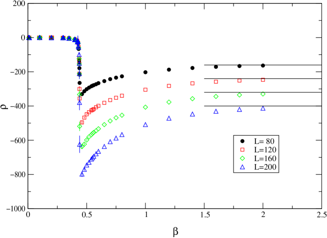
Figure 1: $\rho$ as a function of $\beta$ for different lattice sizes. Continuous lines refer to low temperature calculations.

We have investigated lattices of size $L\times 2L$, with the spatial extension $L$ ranging from 80 to 200. In our simulations we chose $n_{1}=L/2$ and $n_{0}=L$, and periodic boundary conditions were imposed. We simulated both the standard and the kink action of the model by means of a heat-bath algorithm. Errors were estimated by applying the jack-knife method to bunched data. Far from criticality we collected about 100000 measurements for each $\beta$ by sampling each two sweeps; near the critical coupling the statistics has been increased by a factor of 25.

From the behaviour of $\langle\mu\rangle$ in the thermodynamic limit, we expect that $\rho$ is nearly constant at low $\beta$ (due to the slow variation of $\langle\mu\rangle$ in this region), has a sharp negative peak in the critical region (corresponding to the sudden decline of $\langle\mu\rangle$) and approaches $-\infty$ at weak coupling (as a consequence of the restoring of the dual symmetry). The extrapolation of numerical results to the thermodynamic limit should give this behaviour for $\rho$. A plot of $\rho$ data for the lattices we have investigated is reported in Fig. 1. We shall show that the obtained shape of $\rho$ is compatible with the expected behaviour in the infinite volume limit.

By simple algebraic manipulation,

$${\mathcal{D}}(n_{0})=\langle\e^{-\beta(\bar{S}-S)}\rangle_{S}\ ,$$ (32)

where the subscript $S$ means that the average has to be taken over configurations weighted with the standard Ising Boltzmann factor. Only modified links (i.e. links whose sign has been changed) contribute to $\bar{S}-S$, so we get

$${\mathcal{D}}(n_{0})=\langle\e^{-2\beta\sum_{l^{\prime}}\sigma_{i}\sigma_{k}}\rangle_{S}\ ,$$ (33)

where $\sigma_{i}$ and $\sigma_{k}$ are spins connected by a modified link $l^{\prime}$ and the sum is performed over all modified links.

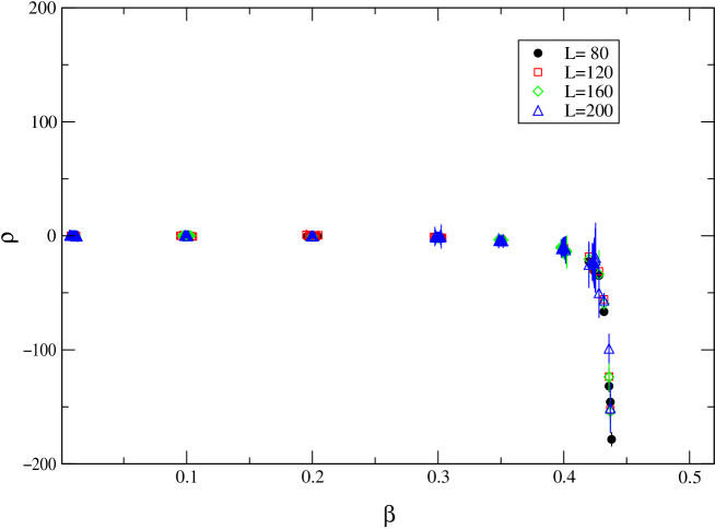
Figure 2: Low $\beta$ data for $\rho$.

In the limit $\beta\to\infty$ the system is completely ordered, so all links are equal to 1 and the sum in Eq. (33) simply reduces to the total number of modified links, i.e.

$${\mathcal{D}}(n_{0})\to\e^{-2\beta L}\ .$$ (34)

Indeed at high $\beta$, $\langle\mu\rangle$ goes to zero in the infinite volume limit, as required from the dual symmetry restoration.

From Eq. (34) we get that

$$\rho\to-2L$$ (35)

at high $\beta$. In Fig. 1 continuous lines indicate the expected results from the high $\beta$ calculation. The agreement with numerical results is evident. We can also consider the opposite implication: if Eq. (35) holds in the weak coupling, in the thermodynamic limit $\langle\mu\rangle=0$ in this region.

On the other hand, $\rho$ is compatible with zero for a wide range of $\beta$’s below $\beta_{\mathrm{c}}$, independently of the volume (see Fig. 2). This implies that $\langle\mu\rangle$ is nearly constant in this region and that feature seems to extrapolate to the thermodynamic limit. Since at high temperature

$$\langle\mu\rangle=1\ ,$$ (36)

our data for $\rho$ imply that $\langle\mu\rangle$ in the thermodynamic limit is different from zero in a wide range of $\beta$’s below $\beta_{\mathrm{c}}$. Hence the behaviour of $\rho$ we obtained is compatible with dual symmetry breaking for $\beta<\beta_{\mathrm{c}}$.

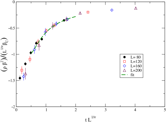
Figure 3: Rescaled plot of $\rho$ data.

In the critical region the approach to the thermodynamic limit is governed by finite size scaling theory, which states that at finite size $L$ in the critical region for $T>T_{\mathrm{c}}$, $\langle\mu\rangle$ is given by

$$\langle\mu\rangle=t^{\delta}f(s)\ ,$$ (37)

with $f$ an unknown function of the scaling variable

$$s=tL^{1/\nu}\ .$$ (38)

From Eq. (37) it follows

$$\rho_{\textrm{rescal}}\equiv\frac{\rho\beta^{2}}{L^{1/\nu}\beta_{\mathrm{c}}}=-\frac{4\delta}{s}-\frac{4}{f(s)}\frac{\d}{\d s}f(s)\ ,$$ (39)

i.e. the rescaled variable $({\rho\beta^{2}})/({L^{1/\nu}\beta_{\mathrm{c}}})$ is a function of the scaling variable $s$.

A plot of rescaled data is shown in Fig. 3. According to Eq. (39), all points should fall on one single curve. We observe however deviations at small and large $s$. It is important to understand the range of validity of Eq. (39). On the one hand, in order for Eq. (26) to be valid, the antikink should be placed at a large temporal distance from the kink. This means that

$$n_{0}=L\gtrsim\xi,$$ (40)

where $\xi$ is the correlation length at a certain temperature. On the other hand, we want to be in the scaling region where finite size scaling is valid, so $L/\xi$ should not take very large values. In order to have an approximate idea, we computed the correlation length in a large $L\times L$ lattice, $L=400$, at the values of $\beta$ used to obtain Fig. 3. The results are shown in Table 1.

$\beta$	$\xi$	Lattices with scaling
0.432	29.1(3)	80
0.436	52.7(2)	80,120,160
0.437	67.6(2)	80,120,160,200
0.438	92.3(1)	80,120,160,200
0.439	138.9(2)	120,160,200
0.44	238.1(4)	-

Table 1: Correlation length in the $2d$ Ising model measured in a $400\times 400$ lattice at the $\beta$ values used in Fig. 3. The third column indicates the lattice sizes which are expected to show scaling behaviour (see text).

The condition Eq. (40) means that, for example for the $L=80$ lattice, only the points of $\beta\lesssim 0.438$ from the list shown in Table 1 should give a proper scaling of $\rho$. On the other hand, $L$ should not be much more larger than $\xi$, because otherwise we go out from the finite size scaling region. We can tentatively write $L/\xi\lesssim 3$, though this value is somewhat arbitrary. In this case this choice corresponds to eliminate the final four points in Fig. 3. Condition (40) eliminates the five points closer to $s=0$ in that figure. Putting the two conditions together, the resulting lattices which should show a proper scaling are given in the third column of Table 1. These are the middle section, 6th-20th points in Fig. 3, which indeed seem to lie on a single curve.

As a further check, we can fit the critical exponent $\delta$ by means of Eq. (39) using as an input $\nu$ and $\beta_{\mathrm{c}}$ ($\nu=1$, $\beta_{\mathrm{c}}=0.44068...$). For the unknown term depending on $f(s)$ we have several possibilities. We can guess that it is roughly constant inside the range of the explored $s$, and do the fit to (fit (a))

$$\rho_{\textrm{rescal}}=-\frac{4\delta}{s}\ ,$$ (41)

or consider that when $s\to 0$, both $f(s)$ and its derivative go to a constant, and write (fit (b))

$$\rho_{\textrm{rescal}}=-\frac{4\delta}{s}+C\ ,$$ (42)

where $C$ is a constant term. We can finally use the three-parameter fit (fit (c))

$$\rho_{\textrm{rescal}}=-\frac{4\delta\,(s+a)}{(s+a)^{2}+b^{2}}\ .$$ (43)

	Fit (a)		Fit (b)		Fit (c)
Points	$\delta$	$\chi^{2}$/DF	$\delta$	$\chi^{2}$/DF	$\delta$	$\chi^{2}$/DF
6-20	0.120(5)	1.42	0.135(2)	1.21	0.132(10)	0.56
7-20	0.120(6)	1.53	0.136(2)	1.22	0.128(9)	0.36
8-20	0.110(3)	0.52	0.143(3)	0.48	0.120(13)	0.36

Table 2: Different fits to obtain the $\delta$ exponent from Eqs. (41)–(43) (see text).

The results of the fits are given in Table 2. Eliminating the 6th or the 7th point (second and third rows in Table 2) corresponds to taking Eq. (40) as a rigourous inequality, $L>\xi$, according to the data of Table 1. Fit (c) gives the more stable values with respect to the modification of the number of points in the fit, and also those with less $\chi^{2}$ by degree of freedom (DF). A mean of the values given by the fit (c) (third column in Table 2) gives $\delta=0.127(8)$, in fair agreement with the expected value $\delta=0.125$. This fit for points 7-20 is shown in Fig. 3.

A more complicated fit allowing also the determination of $\nu$ and $\beta_{\mathrm{c}}$ in principle is also possible, but an appropriate guess of the form of $f$ is needed (see [6, 7, 8]). This fit is useful when only approximated values of $\beta_{\mathrm{c}}$ and $\nu$ are known. In our case the solution of the model is known and the simple quality of the scaling is itself a good indication of the correctness of the approach. We note however that in order to obtain an accurate result for the critical exponents, one should not approach very much the critical point, where the correlation length diverges, in contrast with ordinary analyses. This can be taking into account by monitoring the correlation length, as we showed in this simple case.

4 Conclusions

The analysis of the Ising model suggests that the study of $\rho$ is suitable for investigating order-disorder phase transitions from a dual point of view. While $\langle\mu\rangle$ is not adequate for numerical simulations, $\rho$ data are completely reliable and allow an unambiguous reconstruction of the shape of $\langle\mu\rangle$. In addition, from a finite size scaling analysis we can get the critical exponent associated to the disorder parameter, the critical temperature and the critical exponent of the correlation length, though a careful analysis for this observable is convenient in order to get an accurate measure for the critical exponents.

This analysis is the first complete test of the procedure used to demonstrate that dual superconductivity of the vacuum is the mechanism of colour confinement. The result of this test confirms the hypotheses that are at the basis of the study of Ref. [9].

References

- [1] H.V. Kramers and G.H. Wannier, Phys. Rev. 60 (1941) 252.
- [2] L.P. Kadanoff and H. Ceva, Phys. Rev. B 3 (1971) 3918.
- [3] J. Frölich, P.A. Marchetti, Commun. Math. Phys. 112 (1987) 343.
- [4] L. Del Debbio, A. Di Giacomo, G. Paffuti, Phys. Lett. B 349 (1995) 513.
- [5] L. Del Debbio, A. Di Giacomo, G. Paffuti, P. Pieri, Phys. Lett. B 355 (1995) 255.
- [6] A. Di Giacomo, G. Paffuti, Phys. Rev. D56 (1997) 6816.
- [7] G. Di Cecio, A. Di Giacomo, G. Paffuti, M. Trigiante, Nucl. Phys. B489 (1997) 739.
- [8] A. Di Giacomo, D. Martelli, G. Paffuti, Phys. Rev. D60 (1999) 094511.
- [9] A. Di Giacomo, B. Lucini, L. Montesi, G. Paffuti, Phys. Rev. D 61 (2000) 034504; Phys. Rev. D 61 (2000) 034505.
- [10] E. Marino, B. Schroer, J.A. Swieca, Nucl. Phys. B 200 (1982) 473.
- [11] L. Onsager, Phys. Rev. 65 (1944) 117.