VORTICES AND CONFINEMENT IN
HOT AND COLD D=2+1 GAUGE THEORIES

A. Hart^a, B. Lucini^b, Z. Schram^c and M. Teper^b

^aDepartment of Physics and Astronomy, University of Edinburgh,
Edinburgh EH9 3JZ, Scotland, UK
^bTheoretical Physics, University of Oxford, 1 Keble Road,
Oxford OX1 3NP, England, UK
^cDepartment of Theoretical Physics, University of Debrecen,
H-4010 Debrecen P.O.Box 5, Hungary

Abstract.

We calculate the variation with temperature of the vortex free energy in D=2+1 SU(2) lattice gauge theories. We do so both above and below the deconfining transition at $T=T_{c}$. We find that this quantity is zero at all $T$ for large enough volumes. For $T<T_{c}$ this observation is consistent with the fact that the phase is linearly confining; while for $T>T_{c}$ it is consistent with the conventional expectation of ‘spatial’ linear confinement. In small spatial volumes this quantity is shown to be non-zero. The way it decreases to zero with increasing volume is shown to be controlled by the (spatial) string tension and it has the functional form one would expect if the vortices being studied were responsible for the confinement at low $T$, and for the ‘spatial’ confinement at large $T$. We also discuss in detail some of the direct numerical evidence for a non-zero spatial string tension at high $T$, and we show that the observed linearity of the (spatial) potential extends over distances that are large compared to typical high-$T$ length scales.

1 Introduction

The idea that vortices are the relevant degrees of freedom for understanding confinement in non-Abelian gauge theories is an old one [1]. Consider, for example, an arbitrary SU(2) gauge field, $\{A_{\mu}(x)\}$, in three dimensional Euclidean space-time. Now suppose that we perform the following gauge transformation $\{A\}\to\{A^{g}\}$. Choose a space-like plane and choose a point $x_{c}$ in that plane. Consider any closed loop that encloses that point. We perform a gauge transformation such that, as we go around that closed loop, the gauge transformation varies from $1$ to a non-trivial element of the centre of the group: in this case $z=-1$. Clearly this gauge transformation is not single-valued; nonetheless the gauge potential is, because it is in the adjoint representation. However any field in the fundamental representation would acquire a factor of $-1$; in particular, the Wilson loop defined on such a closed curve, $c$, will acquire a factor of $-1$ relative to its value prior to the gauge transformation

$$W_{c}[A^{g}]=Tr\ e^{\int_{c}A^{g}\cdot ds}=-W_{c}[A]$$ (1)

We extend this construction to all space-like planes, so that the point $x_{c}$ traces a line and we shall refer to this as the vortex (world) line. We can easily generalise the construction so that this line may be closed rather than infinite. If the closed curve along which the Wilson loop is defined links once with the vortex line, then the Wilson loop will acquire a factor of $-1$. If it links $N$ times then it acquires a factor of $(-1)^{N}$. One can consider the field $\{A^{g}\}$ to be the original field $\{A\}$ with an added ultraviolet centre vortex, whose core coincides with the vortex line. Along this line the gauge transformation is singular and the gauge potentials are ill-defined. Since such a vortex corresponds to a gauge transformation everywhere except along a line, we can readily define fields with any number of such vortices (since the problematic vortex intersections will have measure zero). And it is then straightforward to show, as we later shall, that if the vacuum contains an uncorrelated gas of arbitrarily long vortices then the average value of a Wilson loop bounded by a planar curve $c$, will decay as the exponential of its (minimal) area, ${\cal A}[c]$,

$$\langle W_{c}\rangle\propto\exp\{-\sigma{\cal A}[c]\}$$ (2)

with the resulting string tension, $\sigma$ being proportional to the average number of vortex lines threading each unit of area.

When the theory is regularised, such an ultraviolet vortex will become well-defined but will have a divergent action density along the actual vortex line. For example, consider a cubic lattice with a plaquette action. If we place the vortex line so that it avoids all sites and links, then the field is clearly well-defined everywhere. However the plaquettes threaded by this line will have their signs flipped, and this will correspond to an action density along the vortex line, that diverges as we approach the continuum limit. Quantum fluctuations and renormalisation will presumably lead to the line spreading into a tube of finite width, with a non-zero but finite action density within this vortex ‘core’. Indeed, at the classical level we would expect this core to spread to fill the whole box: in which case such a vortex ceases to be a useful degree of freedom. However it may be that quantum fluctuations induce an effective potential for these vortices such that the core is stabilised with a width given by some characteristic length scale. Moreover if this potential is such that these vortices also condense into the vacuum, then they will produce linear confinement between particles in the fundamental representation. But all this is, of course, not guaranteed; if, for example, the vortices are themselves confined, then they will not disorder large Wilson loops.

Whether such vortices exist and, if so, whether they condense, are thus the important dynamical questions for this approach to confinement. They are also difficult non-perturbative questions that have begun to be addressed, during the last two years, in a number of lattice Monte Carlo studies. (See, for example, [2, 3] and references therein.)

Linear confinement corresponds to an area decay, as in (2), for arbitrarily large Wilson loops. If a vortex is to disorder such a loop it must pierce the minimal area an odd number of times and this implies that the vortex line must be correspondingly long. (Unless it is close to the perimeter.) That is to say, one needs a condensate of arbitrarily long vortex lines. Actually this is only so at $T=0$. At high $T$ the requirement becomes far less severe. A vortex that closes upon itself through the periodic temporal direction, is only of length $O(1/T)$ and yet can disorder spatial Wilson loops that are arbitrarily large. (It will not disorder Wilson loops that lie in a space-time plane, but that is to be expected in the high-$T$ deconfining phase.) If vortices exist at all then there will surely exist a finite density of such periodic vortices in the high-$T$ (Euclidean) vacuum. That such short periodic vortices might be the dynamics underlying the apparent area decay of spatial Wilson loops at high $T$ is an old idea. However if the interactions between these vortices were such that they totally screened each other, or were confined, then they would not disorder large spatial loops. That something like this might be the case has been claimed by a recent study [4, 5] of the properties of the magnetic centre symmetry at low and high $T$. This study also suggests that the high-$T$ spatial string tension is only apparent, and that on appropriately large length scales the effective spatial string tension will vanish.

The present work was originally motivated by these [4, 5] unconventional claims. We set out to perform lattice Monte Carlo calculations to determine the properties of the short periodic vortices at high $T$ and to determine whether the spatial string tension was indeed non-zero. The claims made in [4, 5] are strongest for D=2+1 gauge theories and so these are the theories we consider. We work with the simplest SU(2) non-Abelian gauge theory. Our work has, so far, involved a careful reanalysis of some earlier, partially unpublished calculations [6] of the spatial string tension as a function of $T$, together with some simple probes of vortex properties. The results are striking and, if taken at face value, appear to disagree with the suggestion of [4, 5] concerning the behaviour of vortices and spatial confinement at high $T$. Rather they provide some quantitative evidence that vortices at low $T$ and (timelike) periodic vortices at high $T$ have a very similar dynamics. Our work may also be viewed as complementing recent calculations [3] concerning the vortex free energy in D=3+1 low-$T$ SU(2) gauge theories.

2 SU(2) lattice gauge theory in 2+1 dimensions

We work on a cubic lattice with gauge fields represented by SU(2) matrices, $U_{\mu}(n)$, on the links of the lattice. We use the standard plaquette action

$$S=\sum_{p}(1-\frac{1}{2}TrU_{p})$$ (3)

where $U_{p}$ is the ordered product of link matrices around the plaquette labelled $p$. This action appears in the partition function as

$$Z=\int\prod_{l}dU_{l}\exp\{-\beta S\}$$ (4)

where

$$\beta=\frac{4}{ag^{2}}.$$ (5)

This relation holds in the continuum limit and we use it to define $g^{2}$ at arbitrary values of the lattice spacing $a$. (Note that in 3 dimensions the gauge coupling $g^{2}$ has dimensions of mass.) It is clear from (5) that the continuum limit $a\to 0$ corresponds to $\beta\to\infty$. This reflects the fact that the theory becomes free at short distances, just as in 4 dimensions.

To study the theory at finite temperature we use a $L^{2}\cdot L_{t}$ lattice, where $L_{t}$ is the number of sites in the periodic ‘temporal’ direction, and $L\to\infty$ in the thermodynamic limit. The temperature of the system is given by

$$aT=\frac{1}{L_{t}}.$$ (6)

This lattice theory has been studied in detail in recent years [7] and we summarise here some features that will be useful for us later on.

2.1 the confining phase at low $\bf T$

The theory is linearly confining at low $T$. The numerical evidence for this is no less clear-cut than in 3+1 dimensions. The $T=0$ string tension [7] can be accurately parameterised as

$$a\surd\sigma=\frac{1}{\beta}\biggl{\{}1.337+\frac{0.945}{\beta}+\frac{1.10}{\beta^{2}}\biggr{\}}\ \ \ \ \ \ \ :\beta\geq 3.0$$ (7)

with an error of about $\pm 1\%$. We can use (5) to convert (7) into an expression for the dimensionless ratio $\surd\sigma/g^{2}$ in terms of powers of $ag^{2}$. When we need a value of $a\surd\sigma$, or of $\surd\sigma/g^{2}$, at a value of $\beta$ at which direct calculations [7] do not exist, we shall use (7).

An alternative physical mass scale for the theory is provided by the mass gap, $m_{G}$, which, here, turns out to be the mass of the lightest $J^{PC}=0^{++}$ state. An accurate parameterisation for the ratio of $m_{G}$ to $\surd\sigma$ [7] is given by

$$\frac{m_{G}}{\surd\sigma}=4.718-\frac{1.083}{\beta^{2}}\ \ \ \ \ \ \ :\beta\geq 3.75$$ (8)

with an error of $\leq\pm 1\%$ for $\beta\geq 6$ and somewhat larger at lower $\beta$. Using (5) and (7) we can convert (8) into an expression for $am_{G}$ or $m_{G}/g^{2}$.

2.2 the deconfining transition at $\bf T=T_{c}$

As the temperature of the system is increased, the theory undergoes a second order deconfining phase transition at $T=T_{c}$. (See e.g. [8, 9].) The values of $T_{c}$ in [8] can be accurately parameterised by

$$\frac{\beta}{4}\cdot aT_{c}\equiv\frac{T_{c}}{g^{2}}=0.3875\cdot\biggl{(}1-\frac{0.37}{\beta}\biggr{)}^{-1}$$ (9)

which can be translated into a critical value of $L_{t}$

$$L_{t}^{c}(\beta)=\frac{1}{1.55}(\beta-0.37).$$ (10)

We will use (9) and (10) to express the value of $T=1/aL_{t}$ in units of $T_{c}$, at the value of $\beta$ at which we are working.

2.3 the deconfined phase at high $\bf T$

In the deconfined phase, $T>T_{c}$, a Wilson loop defined in a space-time plane will not decay exponentially with its area. However it has long been believed that purely spatial Wilson loops do continue to show an area decay as in (2). That is to say, in the deconfined phase one has ‘spatial’ linear confinement with a corresponding non-zero string tension, $\sigma(T)$, that will depend on the temperature. A number of numerical studies have served to confirm this expectation (see [10] for a recent example), although it is probably fair to say that the effort put into this question has been very much less than that put into the study of confinement at $T=0$. This perhaps leaves room for the suggestion made in [4, 5] that there is in fact no spatial confinement at high $T$ and the apparent spatial area decay is illusory.

Let us consider how this might be. The straightforward possibility is that (accurate) numerical calculations have not been performed on distances that are larger than the relevant dynamical length scale, and so the apparent area decay simply reflects an approximate ‘accidental’ linearity in the spatial potential at small/intermediate distances. An ‘accidental’ linearity is far from impossible. After all, the approximate linearity observed in the $T=0$ potential extends down to distances well below the characteristic distance scale $\sim 1fm$ at which one would have expected a flux tube to have started forming. Thus, the usual heavy-quark potential may be regarded as being ‘accidentally’ linear at small distances. What are ‘small distances’ here? If $T$ is close to $T_{c}$ then

$$\xi_{c}\equiv 1/T_{c}$$ (11)

might be a relevant distance scale. At higher $T$ (see [11] for a review) we expect perturbation theory (in the dimensionless coupling $g^{2}/T\ll 1$) to be good, so that dynamically generated masses are $m^{2}\sim g^{2}T$, and hence a typical dynamical length scale will be

$$\xi_{T}\equiv 1/gT^{1/2}.$$ (12)

However this ignores the infrared divergences in perturbation theory. For example, the Debye screening mass $m_{D}$ is infinite at one loop. Fortunately direct numerical calculations of $m_{D}$ exist [11] and these provide a reference scale

$$\xi_{D}\equiv 1/m_{D}.$$ (13)

We will consider these scales when we come to discuss numerical results on the spatial string tension.

An alternative and more subtle possibility is provided by the actual situation in QCD and similar theories where non-Abelian gauge fields are coupled to fundamental matter fields [12]. Here direct numerical calculations of the potential typically find it to be linearly rising even beyond the distance at which one expects the string to break, and it requires a sophisticated mixing analysis to ‘see’ the string breaking [12]. In such theories the breaking of the string is analogous to the decay of a resonance. The string state exists, but as an unstable state rather than as an asymptotic state. In QCD the decay width is small and so the overlap of a good string operator onto the decay products will be too small for the breaking to be visible in a calculation of limited accuracy. This scenario requires an underlying confinement mechanism that is weakly broken, as in QCD. If there is no confinement to start with, as in weakly coupled D=3+1 QED, then this scenario is irrelevant and there is no sign of any linearity in the potential. While we are not aware of any underlying high-$T$ spatial confinement that would make the QCD example relevant to the discussion of [4, 5], if it were to be so, then the fact that the string breaking is a weak effect should make it easy to identify states into which it decays. For example, in the case of QCD it is into a light $q{\bar{q}}$ pair plus the static sources. Then a mixing analysis [12] could be performed to demonstrate the string breaking.

3 The spatial string tension for $\bf T>T_{c}$

In this section we shall analyse one particular calculation [6] of the spatial string tension in the deconfined phase. We shall look closely at the distance scales over which we see linear confinement and ask whether these distances are ‘large’ or ‘small’. We shall also discuss the values and behaviour of $\sigma(T)$, since, later on in the paper, we shall wish to compare our results with theoretical expressions that incorporate such a spatial string tension.

We shall need to discuss the results of [6] in some detail for two reasons. The first is that some of what we present here has not been previously published. The second is that [6] was not overtly interested in finite temperature physics and a careful translation of notation is needed. The relevant calculations in [6] were performed on $L_{1}\times L_{2}\times L_{3}$ lattices. The Polyakov loops were along the 2 direction and hence the periodic flux tubes onto which they projected were of length $L_{2}$. The correlations were taken in the 1 direction. The value of $L_{3}$ was varied and flux tube masses were obtained for various values of $L_{3}$ and $L_{2}$. In [6] $L_{3}$ was labelled $L_{\perp}$ and was referred to as a transverse spatial direction: the point of the calculation being to estimate the intrinsic width of the confining flux tube. If we choose instead to call $L_{t}\equiv L_{3}$ the Euclidean time direction then what is calculated in [6] is the mass, $M_{p}$, of a spatial confining flux tube of length $L\equiv L_{2}$ at a temperature of $aT=1/L_{t}$. From this we can extract $\sigma(T)$ in the standard fashion:

$$aM_{p}=a^{2}\sigma(T)L-\frac{\pi}{6}\cdot\frac{1}{L}$$ (14)

where the second term on the RHS is the universal string correction for Polyakov loops. These calculations used Polyakov loops separated in the 1-direction and individually smeared in a 2-3 plane. The smearing, however, is only a device for improving the efficiency of the calculation. The lightest flux tube mass is the same as one gets with unsmeared Polyakov loops. And this should give the same string tension as one gets with a large Wilson loop in the 1-2 plane, once the different string corrections have been taken into account.

3.1 linear confinement?

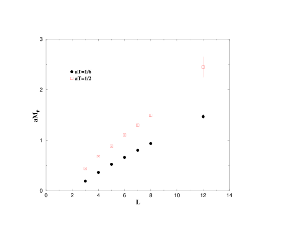
Figure 1: The mass of the spatial flux ‘tube’ versus its length for $aT=1/2>aT_{c}$ ($\Box$) and for $aT=1/6<aT_{c}$ ($\bullet$). All in lattice units at $\beta=4.5$.

The calculations in [6] were performed at $\beta=4.5$ and at $\beta=9.0$. What evidence do we have for linear confinement? Linear confinement will, of course, be reflected in an approximate linear rise in the flux tube mass, $M_{p}$, with its length, $L$. In Fig.1 we show how, at $\beta=4.5$, this mass varies as the flux tube length varies from $L=3$ to $L=12$. We show this for two different values of $L_{t}$. The first is for $L_{t}=2$ which corresponds to a temperature of $T=1/2a=1.33\times T_{c}$ (using (6) and (10)), which is well in the high-$T$ deconfined phase. The second is for $L_{t}=6$ which is well in the low-$T$ confined phase. We see an approximately linear rise throughout this range of $L$, for both values of $T$.

Consider, in more detail, the $L_{t}=2$ high-$T$ calculation. The accurately calculated values are for $L\leq 8$. (The $L=12$ mass is so heavy that the errors become large.) Is a length of $8a$, at $\beta=4.5$ and at $T=1.33T_{c}$, large or small? Now the dynamical scales defined in (11), (12) and (13) are, here, $\xi_{c}\simeq 2.7a$, $\xi_{T}\simeq 1.5a$ and $\xi_{D}\simeq 2.7a$. (For the last relation we have used the value $am_{D}=0.373(5)$ which was calculated in [8] for $\beta=4.5$ and $aT=1/2$, but which was not published.) Compared to these length scales we can confidently claim to have seen linear spatial confinement over ‘large’ distances.

Of course the $\beta=4.5$ calculations correspond to a rather coarse lattice spacing. At $\beta=9$, on the other hand, the lattice spacing is well into the weak coupling scaling region [7] and here there exist calculations [6] of flux tube masses for two lengths, $L=8$ and $L=16$. One again observes an approximate linear rise at both low and high $T$. For example, at $L_{t}=4$ (where $T\simeq 1.4T_{c}$) one finds $aM_{p}(L=8a)=0.292(3)$ and $aM_{p}(L=16a)=0.677(6)$. If we evaluate the previously discussed high-$T$ dynamical length scales at this $\beta$ and $L_{t}$, we find $\xi_{c}\simeq 5.6a$, $\xi_{T}\simeq 3a$ and $\xi_{D}\sim 5a$. (For the last relation we do not have a directly calculated value of $m_{D}$ and have instead interpolated between ‘neighbouring’ values calculated in [11] and unpublished work from [8].) So here too we can claim to have seen linear spatial confinement on reasonably ‘large’ distance scales.

From the above we feel able to say that the spatial linear confinement we observe is not an accidental linearity obtained over small distance scales. On the other hand, the possibility of a weak string-breaking is something we cannot address without a more specific scenario for the string-breaking dynamics.

3.2 $\bf\sigma(T)$

We take from [6] the values of the flux tube mass, $M_{p}$, at $\beta=9$, for various values of the temperature $aT=1/L_{t}$ and for a flux tube length of $L=16a$. We then use (14) to extract the corresponding string tensions, $\sigma(T)$, which we plot in Fig.2. We see that $\sigma(T)\propto T$ for $T>T_{c}$, just as one expects from the simplest dimensional reduction arguments. (This observation, in a different notation, was already made in [6] and a simple dynamical reason for it was given there.) More specifically we find:

$$\sigma(T)\simeq 0.40g^{2}T\simeq T_{c}T\ \ \ \ \ \ \ \ :\ T>T_{c}.$$ (15)

At $\beta=4.5$ only the $L_{t}=2$ calculation is in the deconfined phase, so we cannot perform a similar calculation there. However if we assume a linear rise in $T$ then we obtain a coefficient of $\simeq 0.44$ rather than the $0.40$ in (15). The size of the difference is consistent with being a $O(1/\beta)$ lattice correction and, if so, this implies that the continuum value of the coefficient will be $\simeq 0.36$. Clearly, a more detailed calculation to control the continuum limit would be useful.

In a later section we shall need a particular value of the string tension:

$$a^{2}\sigma(T=1/4a)=0.0443(4)\ \ \ \ \ \ :\beta=9.0.$$ (16)

4 Vortices and boundary conditions

4.1 centre vortices on an infinite lattice

Consider an arbitrary gauge field, $\{U_{\mu}(n)\}$, on an infinite lattice. Let the sites be labelled by integers $(n_{x},n_{y},n_{t})$. We can add an ultraviolet vortex to this field by the following transformation on the fields, $U\to U^{\prime}$. Choose some particular integers $n^{v}_{x},n^{v}_{y}$ which will label the spatial plaquette threaded by the vortex line. We take $U^{\prime}_{l}=U_{l}$ for all links $l$ except that

$$U^{\prime}_{y}(n_{x},n^{v}_{y},n_{t})=-U_{y}(n_{x},n^{v}_{y},n_{t})\ \ \ \ \ {\rm for}\ n_{x}\leq n^{v}_{x}\ {\rm and}\ \forall n_{t}.$$ (17)

It is easy to see that this transformation flips the sign of the spatial $(x,y)$ plaquettes emanating from the sites $(n^{v}_{x},n^{v}_{y},n_{t})$, for all values of $n_{t}$, but that it leaves all other plaquettes unchanged. (Since $-1$ is an element of the centre of the group and so commutes with all $U_{l}$.) Moreover if we consider an arbitrary spatial Wilson loop, it is either unchanged or its sign is flipped. The latter happens if and only if the Wilson loop encircles a plaquette whose sign has been flipped. This has all the expected properties of a vortex. It is an ultraviolet vortex because the vortex core, where the action has changed, is a string of elementary plaquettes. The change of sign of these plaquettes means that their average action has increased; and that the action density along the string will diverge in the continuum limit. The associated $Z_{2}$ gauge transformation has also been localised onto an ultraviolet length scale: a single link. Such a vortex may be suppressed by its action, but the measure of the transformed field is clearly the same as that of the original field.

In the above construction there is a half-plane of links that acquires a minus sign. This half-plane can be smoothly deformed while keeping the edges fixed. On an infinite lattice one edge is invisibly far, and we can deform a set of $\mu=y$ negative links heading off to $n_{x}=-\infty$ to, say, a set of $\mu=x$ negative links heading off to $n_{y}=-\infty$. On a finite lattice this will no longer be possible.

It is also clear that we can introduce any number of these ultraviolet vortices, with vortex lines at any positions. By allowing $n^{v}_{x},n^{v}_{y}$ to vary smoothly with $n_{t}$ we can introduce vortices whose world lines are not straight. A suitable pair of such vortices can produce a vortex line that is a closed loop in space-time. Thus an ensemble of ultraviolet vortices may consist of closed loops of arbitrary sizes and shapes.

When quantum fluctuations are included, we expect that if vortices do exist then the core will acquire a size $O(\xi)$ where $\xi$ is an appropriate dynamical length scale. (And that in any case the gauge transformation will typically be spread over distances greater than one link.) However any such field can be reached by a smooth deformation of the ultraviolet vortex we have defined above, and so, for the ‘kinematic’ part of our discussion, it suffices to focus on the latter.

4.2 twisted and periodic boundary conditions

From now on we shall be in a finite spatial volume. Suppose that we are on a torus so that the gauge potentials are periodic in $x$ and $y$, with periods $L_{x}$ and $L_{y}$ in lattice units. If a gauge field $\{U_{l}\}$ is periodic then it is obvious that when we add an ultraviolet vortex, as in (17), then the transformed field $\{U^{\prime}_{l}\}$ is not periodic. However we can add two such vortices, located at say $n^{v1}_{x},n^{v1}_{y}$ and $n^{v2}_{x},n^{v2}_{y}$, since we can deform the two strings of flipped links so that they join the two vortex cores and there is no string of flipped links heading off to $n_{x}=-\infty$. A Wilson loop that encircles both vortices will not flip sign but one that encircles only one, will. Thus a periodic gauge field possesses an even number of such vortices.

To obtain fields with an odd number of vortices we need to impose twisted boundary conditions. We shall do this in the usual way, keeping the boundary conditions periodic but transforming the plaquette action in (3) as follows (see [11] for a review):

$$S_{tw}=\sum_{p\not=p^{\prime}}(1-\frac{1}{2}TrU_{p})+\sum_{p^{\prime}}(1+\frac{1}{2}TrU_{p^{\prime}})$$ (18)

where the set of plaquettes $p^{\prime}$ is specified to be the set of $(x,y)$ plaquettes emanating from some specific spatial coordinates $n^{tw}_{x},n^{tw}_{y}$ at all values of $n_{t}$. That is to say we flip the sign of a particular string of spatial plaquettes in the action, the string closing on itself through the periodic temporal boundary. That this is equivalent to the usual plaquette action with twisted boundary conditions can be shown by making a singular centre gauge transformation followed by a suitable redefinition of field variables.

Consider a field $\{U\}$ that is typical of those that one obtains with the usual plaquette action (3). Now consider the same field, but with respect to the twisted action. The action density is unchanged, except along the line of twisted plaquettes where its sign is flipped. This is just what we would expect if we had added an (ultraviolet) vortex line so as to thread this line of plaquettes. That is to say, we appear to have added a single vortex to the field $\{U\}$, something that we were previously unable to do.

This interpretation becomes clearer if the vortex is not superimposed upon the twisted plaquettes, but is added to $\{U\}$ so that it threads some other line of plaquettes, labelled by $n^{v}_{x},n^{v}_{y}$. We do this, as usual, by multiplying by $-1$ a string of links running off from $n^{v}_{x},n^{v}_{y}$. Now, instead of running this string to the boundary (which would lead to problems with the periodic boundary conditions) let us run it up to $n^{tw}_{x},n^{tw}_{y}$ where the twisted plaquette lies. This will flip the value of the twisted plaquettes. So now the action density of this field with a twist is the same as that of the original field $U$ without a twist, even at the location of the twist, except that the plaquettes at the location of the vortex core have been flipped. This is exactly what we got when we added a single vortex to a field in an infinite volume. Moreover, any Wilson loop enclosing the vortex, but not the twist, will acquire a factor of $-1$ relative to its value in the field $U$. We may think of the twist as adding a vortex source to the system. Alternatively we note that if we choose to trade the twisted action for twisted boundary conditions, then we obtain a string of flipped links from the vortex to the twist and then on to the boundary. But now this presents no problem because if the field $\{U\}$ was periodic, the field with a vortex added satisfies the twisted boundary conditions. Thus the ensemble of fields obtained with a twisted action is just like the ensemble from the simple plaquette action, but with a vortex added or subtracted. If periodic field have even vorticity then twisted fields have odd vorticity.

4.3 vortex free energy, $\bf F_{v}$

Consider a system at temperature $T=1/aL_{t}$. The partition function and free energy are related by

$$\exp\biggl{\{}-\frac{F}{T}\biggr{\}}=Z.$$ (19)

Let $F_{tw}$ be the free energy of the system with a twist, and $F_{nt}$ of the identical sytem with no twist. We define the vortex free energy to be the difference

$$F_{v}=F_{tw}-F_{nt}.$$ (20)

Note that this will not be the free energy of a single vortex, unless the usual vacuum contains no vortices. It is the free energy difference between a system with an odd number of vortices, and a system with an even number.

From (20), (19) and (4) we readily obtain

$$\frac{\partial}{\partial\beta}\biggl{(}\frac{F_{v}}{T}\biggr{)}=\frac{g^{2}}{4L_{t}}\cdot\frac{\partial}{\partial T}\biggl{(}\frac{F_{v}}{T}\biggr{)}=\langle S_{tw}\rangle-\langle S_{nt}\rangle$$ (21)

where $S_{tw}$ is defined in (18), $S_{nt}$ is the usual untwisted action defined in (3), and we transform the derivative with respect to $\beta$ into one with respect to $T$ using the fact that the former is performed at fixed $L_{t}$.

If $F_{v}\not=0$ in the thermodynamic limit ($L_{x},L_{y}\to\infty$) then the vortices certainly do not condense in the vacuum and will not contribute to a linearly confining ‘spatial potential’. This is known to occur for vortices in a space-time plane at high $T$ [11]. In this paper we calculate not $F_{v}$ itself, but rather $\partial/\partial T(F_{v}/T)$ using (21). We shall assume that if the latter is zero, then so is the former (since we see no reason for $F_{v}$ to be exactly linear in $T$). A direct calculation of $F_{v}$ is possible but less straightforward [3].

4.4 action of a single vortex

A single ultraviolet vortex imposed on a gauge field with $U_{l}=1\ \forall l$ will clearly have an action

$$S_{v}=2L_{t}=\frac{2}{aT}.$$ (22)

If the vortex is fat, so that the $\pi$ units of flux are smoothly spread over $A_{v}$ plaquettes, then

$$S_{v}=\sum_{p}(1-\cos\theta_{p})\simeq\frac{1}{2}\frac{\pi^{2}}{A_{v}}L_{t}.$$ (23)

If we are working with fluctuating gauge fields at some value of $\beta$ then in general we expect the vortex action to be modified by a lattice renormalisation factor:

$$S_{v}(\beta)=S_{v}(\infty)\cdot Z_{v}(\beta).$$ (24)

We note that if, for example, $A_{v}\sim(\xi_{D}/a)^{2}=1/(a^{2}\cdot g^{2}T)$ then $\beta S_{v}$ is independent of $a$ or $T$. On the other hand, if the vortex size is not stabilised by quantum fluctuations, it will spread over the whole spatial volume, $L^{2}$, so that

$$S_{v}\simeq\frac{\pi^{2}}{2}\cdot\frac{L_{t}}{L^{2}}\cdot Z_{v}(\beta)\stackrel{{\scriptstyle L\to\infty}}{{\longrightarrow}}0.$$ (25)

In this case the vortex merges into the Gaussian spin-wave contribution and ceases to be a useful degree of freedom. This is indeed what occurs in U(1) lattice gauge theories: the flux is conserved and hence comes in closed loops, but these do not come in vortices of finite area. Although Wilson loops are still disordered, the effect is Coulombic rather than linearly confining.

4.5 domain walls and spacelike vortices at high T

To give substance to the above discussion of vortices, it would be useful to identify a situation where the vortex becomes a real and easily visible excitation, just like a magnetic monopole in the Higgs phase of the Georgi-Glashow model. It turns out that such a situation exists [11]. Consider a spatial volume $L\times L_{\perp}$ at a temperature $T$ close to zero. Suppose also that $L$ is large. If one decreases $L_{\perp}$ from large values, one finds that there is a phase transition at some $L_{\perp}=L^{c}_{\perp}(\beta)$. If in addition the system possesses a spatial twist, then, for $L_{\perp}\ll L^{c}_{\perp}(\beta)$, one finds that there is a single vortex whose world line extends through time, and which close upon itself through the periodic temporal boundary conditions. Moreover the core of this vortex extends right across the short $L_{\perp}$ direction. In the longer $L$ direction it has a size $\propto\surd(\beta L_{\perp})$. As $L_{\perp}\downarrow$ the vortex action density grows as $S_{v}\propto 1/L^{\frac{3}{2}}_{\perp}$ and the probability of any virtual vortex quantum fluctuation rapidly vanishes. Thus, the special spatial geometry drives the system into an effective vortex Higgs phase, in which the vortex appears ‘squeezed’ by the short spatial direction. Apart from this distortion, it is precisely a vortex of the kind we have been discussing.

In [11] the context of these objects was (apparently) quite different, and we need to provide a brief translation. Consider the system described in the previous paragraph. Rename the time direction to be a spatial one and the short $L_{\perp}$ direction to be the temporal one. Then the phase transition of the previous paragraph is simply the deconfining transition, $T_{c}=1/(aL^{c}_{\perp})$, and the squashed vortex is the ‘domain wall’ separating two high-$T$ $Z_{2}$ vacua. (Or, more precisely, it is the world sheet of the string-like boundary that separates the two $Z_{2}$ vacua.) The Polyakov loops on either side of the vortex have a relative minus sign: just as one would expect for a centre vortex. It was briefly pointed out in [11] that these domain walls have a simple interpretation as real vortices in a space-time plane. Renaming axes it becomes a spatial vortex as discussed in the previous paragraph.

5 Vortices and confinement

In this section we shall assume that centre vortices exist at high $T$ and that they are the fluctuations which produce the spatial string tension. We assume (reasonably) that the relevant vortices are the short ones whose world lines close through the temporal boundary and whose length is therefore $1/T$. These vortices will have a typical area $A_{v}$, and a corresponding action, $S_{v}$, as in (23,24). Note that we are talking here of the vortices in the Euclidean field configurations, rather than the vortices that may appear in the eigenstates of the Hamiltonian. Thus $A_{v}$ may depend on $T$.

In the following calculations we shall assume that the vortices are dilute, since it makes the argument simpler. Whether this is actually so is something we shall return to in the next Section when we discuss our numerical results. As long as vortices are uncorrelated at sufficiently large distances, our conclusions will not be qualitatively altered by vortex correlations which, to a first approximation, can be absorbed into a renormalisation of the effective vortex action.

We shall first show how large Wilson loops acquire an area decay in the presence of such a gas of vortices. We shall ask what the observed $T$ dependence of $\sigma(T)$ teaches us about the properties of these vortices. We shall then show how the average action with twist approaches the periodic action as the volume$\to\infty$, and how this approach is directly related to the string tension generated by the gas of vortices. This parallels the well-known results obtained in [1] for $T=0$.

5.1 vortices and the spatial string tension

Consider a spatial Wilson loop defined along a curve $c$ that bounds a minimal area $\cal A$ (in lattice units). Let us calculate its value within a simple gas of vortices. Suppose that the area $\cal A$ is pierced by $n_{v}$ vortices. Assume they are uncorrelated so that the probability is given by a simple Poisson formula

$$P(n_{v};{\cal A})={{(\mu_{0}{\cal A})^{n_{v}}}\over{n_{v}!}}\cdot e^{-\mu_{0}{\cal A}}$$ (26)

where $\mu_{0}$ is the probability of a vortex piercing a unit area. Now each vortex contributes a factor $-1$ to the value of the Wilson loop, so in this simple picture

$$\langle W_{c}\rangle=\langle Tr\ e^{\int_{c}A\cdot ds}\rangle = \sum_{n_{v}}(-1)^{n_{v}}P(n_{v};{\cal A})$$ (27)

$$= \sum_{n_{v}\ even}P(n_{v};{\cal A})-\sum_{n_{v}\ odd}P(n_{v};{\cal A})$$

$$= e^{-2\mu_{0}{\cal A}},$$

where the last relation follows from using (26). That is to say, the gas of vortices produces linear confinement with a string tension $a^{2}\sigma=2\mu_{0}$.

Since we are at high $T$ we expect the relevant vortex world lines to be closed through the short temporal boundary. If their cross-sectional area is $A_{v}$ (in lattice units) then we expect $\mu_{0}$ in (27) to contain a factor $\sim 1/A_{v}$ as well as a factor containing the action (23,24):

$$a^{2}\sigma(T)=2\mu_{0} \sim \frac{2}{A_{v}}e^{-\beta S_{v}}$$ (28)

$$\simeq \frac{2}{A_{v}}e^{-\frac{\beta\pi^{2}}{2A_{v}}\cdot\frac{1}{aT}\cdot Z_{v}(\beta)}.$$ (29)

One uncertainty here is in the integration over spatial translations of the vortex. This will produce, in addition to the factor $1/A_{v}$, a factor, presumably $O(1)$, that depends on the details of the collective co-ordinate calculation. There will also be a factor from the fluctuations around a vortex. As we remarked earlier, a natural length scale at high $T$ is provided by $\xi_{D}=1/\sqrt{g^{2}T}$. If we assume that $A_{v}\propto(\xi_{D}/a)^{2}$ then we find from (29) and (27) that the string tension is

$$a^{2}\sigma(T)=2\mu_{0}=ca^{2}g^{2}T$$ (30)

where $c$ may have a weak $\beta$ dependence from the $Z_{v}(\beta)$ factor. Thus we naturally obtain a spatial string tension that increases linearly with the temperature (as one would expect from naive dimensional reduction). Conversely the observation that $\sigma(T)\propto T$ implies that $A_{v}\propto 1/T$ and hence that the weighting $\exp(-\beta S_{v})$ is independent of $T$.

5.2 $\bf\Delta S$ and vortices

What do we expect for the action difference

$$\Delta S\equiv\langle S_{tw}\rangle-\langle S_{nt}\rangle$$ (31)

that appears in (21)? The only difference between having twisted and periodic boundary conditions on our $L\times L$ spatial volume is that these constrain us to having an odd or even number of vortices respectively. We assume that in both cases we have a Poisson distribution, just as in (26) with ${\cal A}=L^{2}$. Thus the probability of $n_{v}$ vortices is

$$P(n_{v};L^{2})=\frac{1}{\cal N}\cdot{{(\mu_{0}L^{2})^{n_{v}}}\over{n_{v}!}}$$ (32)

where the normalisation factors in the two cases are

$${\cal N}_{tw}=\sum_{n_{v}\ odd}{{(\mu_{0}L^{2})^{n_{v}}}\over{n_{v}!}}=\sinh(\mu_{0}L^{2})$$ (33)

$${\cal N}_{nt}=\sum_{n_{v}\ even}{{(\mu_{0}L^{2})^{n_{v}}}\over{n_{v}!}}=\cosh(\mu_{0}L^{2}).$$ (34)

Let $s_{0}$ be the effective action of a single vortex. Then it is a simple calculation to obtain

$$\Delta S = \frac{1}{{\cal N}_{tw}}\sum_{n_{v}\ odd}n_{v}s_{0}{{(\mu_{0}L^{2})^{n_{v}}}\over{n_{v}!}}-\frac{1}{{\cal N}_{nt}}\sum_{n_{v}\ even}n_{v}s_{0}{{(\mu_{0}L^{2})^{n_{v}}}\over{n_{v}!}}$$ (35)

$$= s_{0}\cdot\mu\frac{\partial}{\partial\mu}\ln(\tanh\mu)$$

$$= 2s_{0}\cdot a^{2}\sigma L^{2}\cdot{{e^{-a^{2}\sigma L^{2}}}\over{1-e^{-2a^{2}\sigma L^{2}}}}$$

where in the second line we use the shorthand notation $\mu\equiv\mu_{0}L^{2}$ and at the final step we have used $2\mu_{0}=a^{2}\sigma(T)$ from (30).

In (35) the overall factor of $\exp\{-a^{2}\sigma L^{2}\}$ is no surprise in a linearly confining theory: it arises from the fact that we are subtracting the partition function for an odd number of vortices from that for an even number, just as in (27). The prefactor of $\sigma L^{2}$ arises from the average number of vortices in the $L^{2}$ volume; both $\langle S_{tw}\rangle$ and $\langle S_{nt}\rangle$ are proportional to it for large volumes; and hence so is their difference, $\Delta S$. For small enough spatial volumes we expect the periodic volume to have no vortices and the twisted volume to have just one vortex. We observe that (35) embodies this expectation: in the limit $L^{2}\to 0$, one obtains $\Delta S\to s_{0}$, since the factor in the denominator cancels the $\sigma L^{2}$ prefactor in the numerator. Of course, for realistic vortices, the action will start to vary once $L^{2}<A_{v}$ and this simple formula will break down.

6 Calculations of $\bf\Delta S$

In this section we present the results of our lattice Monte Carlo calculations of $\Delta S$. This is defined (31) as the difference of the average total action on lattices with and without a twist: $\Delta S\equiv\langle S_{tw}\rangle-\langle S_{nt}\rangle$. It is related (21) to the derivative with respect to $T$ of the vortex free energy $F_{v}$. In the low $T$ deconfining phase we expect that $\lim_{L\to\infty}F_{v}=0$ and hence $\lim_{L\to\infty}\Delta S=0$. If we have spatial confinement at high $T$ then we expect this to hold there as well. At low $T$ there are specific expectations about how this limit is approached [1]. At high $T$ we can test the possibilities described in the previous section.

Our individual calculations of $\langle S_{tw}\rangle$ and $\langle S_{nt}\rangle$ consist, typically, of $O(10^{6}-10^{7})$ interweaved heat bath and over-relaxed sweeps. We shall begin with a calculation of $\Delta S$ in large spatial volumes and for temperatures ranging from well below $T_{c}$ to well above. We shall then present a finite volume study of $\Delta S$ for $T>T_{c}$. We shall finish with a similar finite volume study of the system in the low $T$ confining phase.

6.1 $\bf\Delta S$ on large spatial volumes

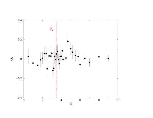
Figure 3: The difference of twisted and untwisted actions on $L_{t}=2$ lattices. $T$ increases as $\beta$ increases, and the system deconfines at $\beta_{c}$ as indicated. The spatial volumes are large in physical units, except very close to $\beta=\beta_{c}$ where there is a diverging correlation length.

Our first calculation is of $\Delta S\equiv\langle S_{tw}\rangle-\langle S_{nt}\rangle$ in the limit of large volumes and for temperatures ranging from values that are well within the confining phase, to values much larger than $T_{c}$. The vortex free energy (21), and hence $\Delta S$, should certainly be zero for $T<T_{c}$, so the interesting question is whether there is a change for $T>T_{c}$. In Fig.3 we show our results. As is clear, these are compatible with $\Delta S=0$ over our whole range of $\beta$. However, to assess the significance of this result, there are some questions that need to be answered. First, what is the range of $T$? Then, how large is the spatial volume? Finally, and most importantly, are the errors on these values of $\Delta S$ small compared to the non-zero value one is attempting to discriminate against?

First, the range of $T$. On our $L_{t}=2$ lattice deconfinement occurs for $\beta=\beta_{c}=3.47$ (see (10)). The range of $\beta$ values for this calculation is $\beta\in[0.5,9.0]$. Using (5,6) this translates into $0.15T_{c}\leq T\leq 2.6T_{c}$. (Note that because of large lattice corrections at small $\beta$, the lower limit has to be interpreted with care.)

Is the volume large? We use $L=12$ for $\beta<2.5$, $L=16$ for $2.5\leq\beta<4.5$, and $L=24$ for $\beta\geq 4.5$. First consider $T<T_{c}$, i.e. $\beta<3.47$. Here a relevant physical length scale is provided by $\xi_{\sigma}\equiv 1/\sigma(T=0)$. In these units [7] we have $aL/\xi_{\sigma}>7.8$ for $T<T_{c}$. As $T\to T_{c}$ there is a correlation length, $\xi_{p}$, that diverges (the transition is second order) and so there will be some region of $\beta$ near $\beta_{c}$ where our volume will become too small to accommodate $\xi_{p}$. Such finite volume effects have been studied in detail in [8] and one finds that they become significant on a $16^{2}2$ lattice only for $\beta>3.15$ where $\xi_{p}>7$. Going now to $T>T_{c}$ we note that there is again an interval close to $T_{c}$ where the correlation length diverges. We do not have direct calculations of finite size effects here, but we assume that they are negligible for $\beta\geq 3.7$ since $\xi_{p}(\beta=3.7)\simeq 3$ and $\xi_{D}(\beta=3.7)\simeq 6$ [8]. In the high-$T$ range our lattice sizes range from $aL\sim 4.5\xi_{D}$ at $\beta=4.0$ to $aL\sim 9\xi_{D}$ at $\beta=9.0$. Thus, apart from a window of temperatures close to $T_{c}$, the volumes we are using are indeed large. (In fact there is some reason to believe that even within this window the quantities we are interested in will be little affected. For example, the calculated values of the spatial string tension, $\sigma(T)$, show no effects as $T$ passes near $T_{c}$. And we see no sign of larger fluctuations near $T_{c}$ in either $\sigma(T)$ or $\Delta S$.) We shall later perform some detailed finite volume studies that will confirm this.

How significant is our result that $\Delta S$ is compatible with zero? The extra action of a single ultraviolet vortex would arise from the change in sign of a single plaquette in each time-slice, and so it would contribute $\delta S_{v}=L_{t}\langle TrU_{p}\rangle$. This increases from $\delta S_{v}\simeq 2.5$ at $\beta=3.0$ to $\delta S_{v}\simeq 3.5$ at $\beta=9.0$. This is certainly excluded by Fig.3. The action of a more realistic ‘fat’ vortex will depend on the area, as in (23) and (24). Our results constrain the diameter of such a vortex to be $d_{v}>10a$. Compared to the natural length scales in the problem (as discussed above) this is very large, and thus we believe that our results for $\Delta S$ strongly discriminate against the twisted system differing from the untwisted one by the presence of a single extra vortex.

6.2 $\bf\Delta S$ as a function of $\bf L$ for $\bf T>T_{c}$

We have seen that $\lim_{L\to\infty}\Delta S=0$. How is this limit approached? Does it point to a gas of confining vortices, and hence a behaviour as in (35)? Or is it just that vortices do not exist; for example as in (25) because their size is not stabilised?

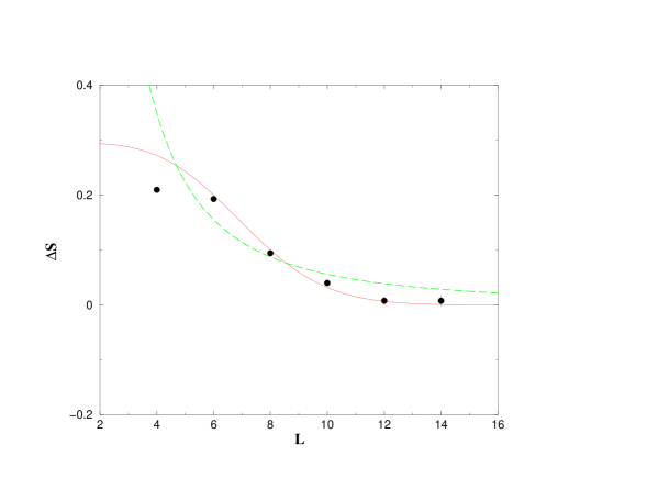
Figure 4: The difference of twisted and untwisted actions at $T=1/4a>T_{c}$ at $\beta=9$, for various spatial sizes. Curves correspond to best fits for a dilute vortex gas (solid line) and for a single unstable ‘vortex’ (dashed line).

To address this question we have calculated $\Delta S$ as a function of the spatial lattice size, $L$, at $\beta=9$ and for $L_{t}=4$ which, at this $\beta$, corresponds (10) to $T\simeq 1.4T_{c}$. We show our results in Fig.4. We observe that on small volumes $\Delta S$ does indeed deviate substantially from zero. Moreover, we see that the variation is not compatible with the $\Delta S\propto 1/L^{2}$ behaviour expected (25) if the ‘vortex’ spreads to fill the whole spatial volume. By contrast it is well fitted by the expression (35) that one derives in a dilute vortex gas. (Except for the smallest lattice, which corresponds to a $4^{3}$ volume, and which can hardly be characterised as a system at a finite $T$.)

As an aside we remark that an equally good fit can be obtained using the expression in (35) without the term in the denominator. Clearly much more accurate calculations will be needed to determine whether it is there or not. We have also tried a fit of the form (25) modified by a screening factor of the form $\exp(-mL)$. This gives a rather poor fit.

Returning to the fit using (35), we find that the parameter in the exponent is constrained to be

$$a^{2}\sigma(aT=0.25)=0.043\pm 0.002.$$ (36)

We note that this is in precise agreement with the value of the spatial string tension, $a^{2}\sigma(aT=0.25)=0.0443(4)$ that we obtained in (16) from Polyakov loop correlations at the same value of $a$ and $T$. This provides a striking confirmation of the simple vortex model.

Can we learn something about the properties of these vortices? For example, if we can estimate the vortex area and also the average density of vortices, then we can determine whether the vortices are indeed dilute. The density is straightforward to determine. From (26,30) the average number of vortices per unit area is

$${\bar{n}}_{v}=\mu_{0}=\frac{a^{2}\sigma(T)}{2}\simeq 0.022$$ (37)

which implies that the typical separation between neighbouring vortices is

$$\delta r=\frac{1}{\surd{\bar{n}}_{v}}\simeq 7$$ (38)

in lattice units. Now, we have previously suggested that the vortex area should be $A_{v}\sim 1/(ag^{2}.aT)\simeq 9$. If so, such a vortex gas will indeed be quite dilute.

It would be much better to estimate $A_{v}$ directly; but this is not so easy because of the unknown factors, such as $Z_{v}(\beta)$. If we ignore these factors then we can obtain wildly different estimates of $A_{v}$. For example, one approach is to take the overall coefficient of the fit in Fig.4

$$2s_{0}a^{2}\sigma=0.024\pm 0.002$$ (39)

and then to use (36) to obtain $s_{0}\simeq 0.27$. If we use this value for $S_{v}$ in (28) we obtain $A_{v}\sim 4$. If instead we use (29) with $s_{0}\simeq 0.27$ then we find $A_{v}\sim 70$. This huge disagreement suggests that these calculations are much too rough to be useful. At a very qualitative level, the fact that (35) fits the values in Fig.4 all the way down to $L=6$, with the same value of the vortex action, does suggest that the vortex is not being squeezed in this range. This suggests that the vortex area satisfies $A_{v}<36$, so that the vortex gas is at least moderately dilute.

6.3 $\bf{\Delta S}$ as a function of $\bf L$ for $\bf{T<T_{c}}$

In the low $T$ confining phase one expects, from the general analysis of [1], that the vortex free energy, $F_{v}$, should approach zero as $L\to\infty$ with a correction that $\propto\exp(-a^{2}\sigma L^{2})$. This is also the prediction of our simple vortex model if we generalise it to a condensate of the arbitrarily long vortex lines that would be needed to disorder arbitrarily large Wilson loops at $T=0$.

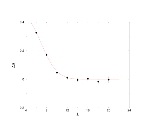
Figure 5: The difference of twisted and untwisted actions at $T=1/6a<T_{c}$ at $\beta=7$, for various spatial sizes. Fit shown is for a dilute vortex gas.

It would obviously be of interest to extend our high-$T$ calculations of $\Delta S$ to low $T$ so as to test these expectations. In Fig.5 we show the result of such a calculation on lattices with $L_{t}=6$ at $\beta=7$. Using (10) we see that this corresponds to $T\simeq 0.7T_{c}$. We also show in the figure a best fit of the form in (35) to the values for $L\geq 6$. This clearly fits very well. From the exponent we extract the value

$$a^{2}\sigma=\left\{\begin{array}[]{ll}0.043(2)&\ \ \ L\geq 6\\ 0.048(4)&\ \ \ L\geq 8\end{array}\right.$$ (40)

This is nicely consistent with the low-$T$ string tension, $a^{2}\sigma\simeq 0.0455$, that one obtains from (7) at $\beta=7$. (The comparison with the $T=0$ string tension is the correct one to make even though $T\not=0$ here. The reason is that the spatial string tension does not vary significantly with $T$ until $T$ is close to $T_{c}$, as we see in Fig.2.)

As a check of the scaling properties of this behaviour, we have also performed such a calculation on $L_{t}=4$ lattices at $\beta=5$. Using (10) we see that this corresponds to $T\simeq 0.75T_{c}$. We again show the best fit of the form (35), in this case to $L\geq 4$. Again this fits very well. From the fits we extract

$$a^{2}\sigma=\left\{\begin{array}[]{ll}0.091(2)&\ \ \ L\geq 4\\ 0.080(7)&\ \ \ L\geq 6\end{array}\right.$$ (41)

which, we note, is reasonably consistent with the string tension, $a^{2}\sigma=0.0979(13)$, that one obtains by a direct $T=0$ calculation [7] at this value of $\beta$.

So we see that in the low $T$ confining phase, the finite volume corrections to the asymptotic $\Delta S=0$ result, are also precisely what one expects from the simple vortex model (and indeed from the more general arguments of [1]). We note that the fact that the functional form fits all the way down to $4^{3}$ and $6^{3}$ lattices at $\beta=5$ and $7$ respectively, is in contrast to the high-$T$ $L_{t}=4$ case where the value of $\Delta S$ on the $4^{3}$ lattice falls below the fit. The temptation is to interpret this as follows. As $L\downarrow$ at fixed $L_{t}=1/aT$, the lattice ceases to correspond to a thermodynamic system at a fixed $T$, and so the area of the vortex begins to grow, as it loses its $\propto 1/T$ suppression factor. This leads to a decrease of $s_{0}$ and hence of $\Delta S$. This is of course no more than a plausible speculation.

7 Conclusions

That centre vortices might drive confinement is an attractive idea [1] which has motivated a number of recent lattice calculations, e.g. [2, 3]. At high temperatures one would naively expect to find a gas of such vortices which, in a Euclidean calculation, would manifest themselves as vortex world lines that close through the short ($=1/T$) temporal boundary. In the deconfining phase these should then provide the mechanism for ‘spatial’ linear confinement. The statistical mechanics of such high-$T$ vortices is relatively simple, as we saw in a calculation that showed how a spatial string tension, $\sigma(T)$, is generated within a dilute gas of vortices. The observed $\sigma(T)\propto T$ behaviour arises naturally if the vortex cross-section has an area $\propto g^{2}T$.

In contrast to such expectations is the recent suggestion [4, 5] that the vortices might not be uncorrelated at large separations, so that there is no linear spatial confinement for $T>T_{c}$. To address this possibility we performed calculations of the variation with $T$ of the vortex free energy and found it to be zero at all temperatures, high and low. This supports the conventional expectation of a non-zero spatial string tension. We then calculated the approach to zero as the spatial volume increases and found that it was controlled by the same spatial string tension, $\sigma(T)$, that had been obtained in earlier direct calculations of that quantity. Moreover the functional behaviour is exactly like the one we derived within the dilute vortex gas. From the fits we estimated the mean inter-vortex distance and, much more roughly, the vortex area. These estimates suggest that the vortices are indeed moderately dilute.

We performed similar calculations in the low-$T$ confining phase and showed that there too the finite volume corrections are as expected for a dilute gas of vortices, although here the argument can be made much more generally [1].

We carefully reanalysed some earlier calculations [8, 6] of the spatial string tension and showed that the observed linearity of the potential extends over distances that are large compared to the natural dynamical length scales at high $T$.

All this provides strong evidence that the usual expectation of an area decay for spatial Wilson loops at high $T$ is indeed correct. It also provides support for the notion that, at least at high $T$, vortices do produce this area law behaviour. We intend to pursue these questions with a better scaling study as well as a dedicated spatial string tension calculation. Such studies are worth pursuing because the dynamics of vortices should be much simpler to identify at high $T$; both in Euclidean calculations and possibly through a careful analysis of the relatively tractable D=1+1 reduced theory.

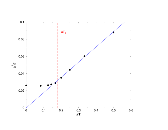
Figure 2: The spatial string tension as a function of $aT$ at $\beta=9$. The deconfining temperature, $aT_{c}$, is indicated.

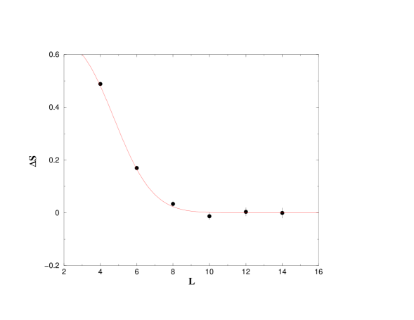
Figure 6: The difference of twisted and untwisted actions at $T=1/4a<T_{c}$ at $\beta=5$, for various spatial sizes. Fit shown is for a dilute vortex gas.

References

- [1] G. ‘t Hooft, Nucl. Phys. B138 (1978) 1; B153 (1979) 141; Cargese Lectures, 1979; Schladming Lectures, 1980.
- [2] M. Faber, J. Greensite, S. Olejnik and D. Yamada, hep-lat/9912002.
- [3] T. Kovacs and E. Tomboulis, hep-lat/0002004.
- [4] C. Korthals-Altes, A. Kovner and M. Stephanov, hep-ph/9909516.
- [5] C. Korthals-Altes and A. Kovner, hep-ph/0004052.
- [6] M. Teper, Phys. Lett. B311 (1993) 223 and unpublished notes.
- [7] M. Teper, Phys. Rev. D59 (1999) 014512.
- [8] M. Teper, Phys. Lett. B313 (1993) 417 and unpublished notes.
- [9] J. Engels et al., Nucl. Phys. Proc. Suppl. 53 (1997) 420.
- [10] P. Bialas, A. Morel, B. Petersson, K. Petrov and T. Reisz, hep-lat/0003004.
- [11] C. Korthals Altes, A. Michels, M. Stephanov and M. Teper, Phys. Rev. D55 (1997) 1047.
-
[12]
I. T. Drummond,
Phys. Lett. B434 (1998) 92; Phys. Lett. B442 (1998) 279.
I. T. Drummond and R. Horgan, Phys.Lett. B447 (1999) 298.
O. Philipsen and H. Wittig, Phys. Rev. Lett. 81 (1998) 4056; Phys. Lett. B451 (1999) 146.
F. Knechtli and R. Sommer, Phys. Lett. B440 (1998) 345.
Ph. de Forcrand and O. Philipsen, hep-lat/9912050.
C. DeTar, U. Heller and P. Lacock, hep-lat/9909078.
P. Pennanen and C. Michael (UKQCD collaboration), hep-lat/0001015.