Domain Wall Fermions with Exact Chiral Symmetry

Abstract

We show how the standard domain wall action can be simply modified to allow arbitrarily exact chiral symmetry at finite fifth dimensional extent. We note that the method can be used for both quenched and dynamical calculations. We test the method using smooth and thermalized gauge field configurations. We also make comparisons of the performance (cost) of the domain wall operator for spectroscopy compared to other methods such as the overlap-Dirac operator and find both methods are comparable in cost.

I Introduction

Recently a great deal of theoretical progress has been made in the construction of lattice regularizations of fermions with good chiral properties [1, 2, 3]. For use in practical numerical simulations, though, approximations to these formulations are necessary. In the formulation using domain wall fermions (DWF) [1, 4], the extent of an auxiliary fifth dimension has to be kept finite in numerical simulations while chiral symmetry holds strictly only in the limit of infinite fifth dimension. The violations of chiral symmetry are expected to be suppressed exponentially in the extent of the fifth dimension [4, 5], but in practice the coefficient in the exponent can be quite small [6, 7] and the suppression correspondingly slow.

In the case of overlap fermions there is no such problem in principle. However, there is a problem of practicality: how to deal efficiently with $\epsilon(H)=H/\sqrt{H^{2}}$, where $H$ is some auxiliary Hermitian lattice Dirac operator for large negative mass, but free of doublers. Most commonly, the Hermitian Wilson-Dirac operator $H_{w}$ is used. So far, the best methods use rational polynomial approximations of $\epsilon(H)$ rewritten as a sum over poles

$$\epsilon(H)=\frac{HP(H^{2})}{Q(H^{2})}=H\left(c_{0}+\sum_{k=1}^{n}\frac{c_{k}}{H^{2}+b_{k}}\right)~{}.$$ (1)

Variants of this are Neuberger’s polar decomposition [8] and the optimal rational polynomial approximation of Ref. [9, 10]. In the application of $\epsilon(H)$ on a vector $\psi$ the shifted inversions $(H^{2}+b_{k})^{-1}\psi$ are done simultaneously with a multi-shift CG inverter [11]. This is referred to as the “inner CG”, since typically another, “outer”, CG method is used to compute propagators or eigenvalues of the overlap Dirac operator containing $\epsilon(H)$.

In these methods, the main problem is the difficulty of getting an accurate approximation to $\epsilon(x)$ for small $x$. As emphasized in Ref. [12, 10] accuracy for the lower range of the spectrum of $H$ can always be enforced by calculating a sufficient number of eigenvectors of $H$ with small eigenvalues and computing $\epsilon(H)$ in the space spanned by these eigenvectors exactly. The approximation is then only used after projecting out these eigenvectors. This is referred to as “projection”.

Small eigenvalues of $H_{w}$ occur quite frequently on (quenched) lattices used in current simulations. Indeed, a non-zero density of eigenvalues near zero has been found [13]. Projection is thus essential in efficient implementations of the overlap Dirac operator. It is known that the zero eigenvalues of $H_{w}$ correspond to unit eigenvalues of the transfer matrix $T$ that describes propagation along the fifth direction for domain wall fermions [2]. The left and right handed physical fermions in the domain wall formulation occur along the two boundaries in the fifth direction. A unit eigenvalue of the transfer matrix then allows for unsuppressed interaction between left and right handed fermions and thus to a breaking of chiral symmetry. Therefore the same modes that make the approximation of $\epsilon(H)$ difficult to achieve in overlap fermions, and need to be projected, are responsible for the chiral symmetry breaking for domain wall fermions at finite $L_{s}$.

If we could project out the modes with near unit eigenvalue of the transfer matrix and take their contribution with effectively infinite $L_{s}$ we could obtain a domain wall fermion action with no chiral symmetry breaking even at finite $L_{s}$. This would make domain wall fermions with finite $L_{s}$ equivalent to overlap fermions. It would then become a matter of computational efficiency as to which form is to be preferred for numerical simulations. Based on ideas of Boriçi [14] we show in section II how projection for domain wall fermions can be achieved. In section III we illustrate how projection works, first on smooth instanton configurations and then on a configuration from a quenched simulation. We discuss the degree of chiral symmetry conservation that can be achieved and compare the performance (cost) of domain wall fermion implementations with and without projection to overlap fermions. We conclude the paper with a brief summary and some discussions in section IV.

II Projected Domain Wall Fermion Actions

Kaplan’s method [1] realizes a single massless fermion field through an infinite tower (or infinite number of flavors) of massive fermion fields with a particular flavor structure. The flavor index can be interpreted as an extra (here fifth) dimension, and the flavor structure as a defect along the fifth dimension to which the massless fermions are bound. Lattice calculations necessarily require a finite fifth dimensional extent and lattice spacing, as well as regularizations for the derivatives in the four dimensional space and in the fifth direction. These regularizations are not unique. In particular, higher order terms in the fifth dimensional lattice spacing can be added to the action, as long as they do not change the “defect structure”. Such changes can affect the effective four dimensional theory by altering the discretization effects in the four dimensional lattice spacing, but not the continuum limit.

The finite fifth dimensional extent induces some chiral symmetry violation. This can be eliminated by “projecting” an appropriate number of violation inducing states. We show how the projection method can be implemented for two different five dimensional domain wall actions. The Wilson fermion action is used for the four dimensional part of the action, but it should be understood that other actions realizing a single massive fermion field could be considered, and much of the following derivations do not depend on the specific form chosen.

A Form of the actions

To fix our notation/conventions, we write the usual, 4-d, Wilson-Dirac operator as

$$D_{w}(M) = (4+M)\delta_{x,y}-\frac{1}{2}\sum_{\mu=1}^{4}\Bigl{[}(1-\gamma_{\mu})U_{\mu}(x)\delta_{x+\mu,y}+(1+\gamma_{\mu})U_{\mu}^{\dagger}(y)\delta_{x,y+\mu}\Bigr{]}$$ (2)

$$= \begin{pmatrix}B+M&C\\ -C^{\dagger}&B+M\end{pmatrix}.$$ (3)

Here, with $\sigma_{\mu}=(\sigma_{k},i{\bf 1})$,

$$C = \frac{1}{2}\sum_{\mu=1}^{4}\sigma_{\mu}\Bigl{[}U_{\mu}(x)\delta_{x+\mu,y}-U_{\mu}^{\dagger}(y)\delta_{x,y+\mu}\Bigr{]},$$ (4)

$$B = \frac{1}{2}\sum_{\mu=1}^{4}\Bigl{[}2\delta_{x,y}-U_{\mu}(x)\delta_{x+\mu,y}-U_{\mu}^{\dagger}(y)\delta_{x,y+\mu}\Bigr{]}.$$ (5)

We are using a chiral basis: $\gamma_{\mu}=\begin{pmatrix}0&\sigma_{\mu}\\ \sigma_{\mu}^{\dagger}&0\end{pmatrix}$, $\gamma_{5}=\begin{pmatrix}1&0\\ 0&-1\end{pmatrix}$. We will also use the hermitian Wilson-Dirac operator

$$H_{w}(M)=\gamma_{5}D_{w}(M)=\begin{pmatrix}B+M&C\\ C^{\dagger}&-B-M\end{pmatrix}.$$ (6)

Usually, we will use a large negative mass here, but often omit the argument from $D_{w}$ and $H_{w}$.

In this notation, the usual domain wall fermion action of Shamir [4] reads, with an explicit fifth dimensional lattice spacing $a_{5}$ for the hopping term — the 4-d lattice spacing $a$ is kept fixed at $a=1$ throughout —,

$$S_{DW}=-\bar{\Psi}D^{(5)}_{DW}\Psi=-\sum_{i=1}^{L_{s}}\bar{\Psi}_{i}\Bigl{\{}\bigl{[}a_{5}D_{w}(-M)+1\bigr{]}\Psi_{i}-P_{-}\Psi_{i+1}-P_{+}\Psi_{i-1}\Bigr{\}}$$ (7)

where the extent of the fifth dimension, $L_{s}$ has to be taken as even. The gauge fields in $D_{w}(-M)$ are independent of the fifth coordinate, and the fermion fields satisfy the boundary conditions in the fifth direction:

$$P_{-}\Psi_{L_{s}+1}=-mP_{-}\Psi_{1},\qquad P_{+}\Psi_{0}=-mP_{+}\Psi_{L_{s}}.$$ (8)

$P_{\pm}$ are the chiral projectors, $P_{\pm}=\frac{1}{2}(1\pm\gamma_{5})$. $0\leq m<1$ is proportional to the quark mass (for small $m$). The 4-d physical fermion degrees of freedom are identified with the fields at the boundaries as

$$q^{R}=P_{+}\Psi_{L_{s}}=\Psi_{L_{s}}^{R}, \quad q^{L}=P_{-}\psi_{1}=\Psi_{1}^{L},$$ (9)

$$\bar{q}^{R}=\bar{\Psi}_{L_{s}}P_{-}=\bar{\Psi}_{L_{s}}^{R}, \quad\bar{q}^{L}=\bar{\psi}_{1}P_{+}=\bar{\Psi}_{1}^{L}.$$ (10)

As will be shown below, projection of low-lying eigenvalues of $-\log T$, with $T$ the transfer matrix along the fifth direction, can be achieved by introducing an additional term in (7) so that the complete domain wall fermion action reads

$$S_{DWP}=-\bar{\Psi}D^{(5)}_{DWP}\Psi= - \sum_{i=1}^{L_{s}}\bar{\Psi}_{i}\Bigl{\{}\bigl{[}a_{5}D_{w}(-M)+1\bigr{]}\Psi_{i}-P_{-}\Psi_{i+1}-P_{+}\Psi_{i-1}\Bigr{\}}$$ (11)

$$+ \qquad\bar{\Psi}_{1}\hat{A}(m)\bigr{[}P_{-}\Psi_{1}+P_{+}\Psi_{L_{s}}\bigl{]}.$$ (12)

Boriçi [14] introduced an interesting variation of the domain wall fermion action, which differs from the usual one by terms of order ${\cal O}(a_{5})$. He called it (5-d) truncated overlap action, since its effective 4-d action for the light fermions is just the polar decomposition approximation of order $L_{s}/2$ to the overlap Dirac operator introduced by Neuberger [8]. In our notation, and introducing again an additional term to be used for projecting low-lying eigenvalues, Boriçi’s variant reads

$$S_{DW^{\prime}}=-\bar{\Psi}D^{(5)}_{DW^{\prime}}\Psi=-\sum_{i=1}^{L_{s}}\bar{\Psi}_{i} \Bigl{\{}\bigr{[}a_{5}D_{w}(-M)+1\bigl{]}\Psi_{i}+\bigr{[}a_{5}D_{w}(-M)-1\bigl{]}P_{-}\Psi_{i+1}+$$ (14)

$$~{}~{}\bigr{[}a_{5}D_{w}(-M)-1\bigl{]}P_{+}\Psi_{i-1}\Bigr{\}}+\bar{\Psi}_{1}\hat{A}(m)\bigr{[}P_{-}\Psi_{1}+P_{+}\Psi_{L_{s}}\bigl{]}.$$

The boundary conditions in the fifth direction remain as in (8). The kernel of the 5-d operator is, including the boundary conditions,

$$D^{(5)}_{DW^{\prime}}=\begin{pmatrix}D_{+}-\hat{A}P_{-}&D_{-}P_{-}&0&0&\cdots&0&0&-mD_{-}P_{+}-\hat{A}P_{+}\cr D_{-}P_{+}&D_{+}&D_{-}P_{-}&0&\cdots&0&0&0\cr 0&D_{-}P_{+}&D_{+}&D_{-}P_{-}&\cdots&0&0&0\cr\vdots&\vdots&\vdots&\vdots&\vdots&\vdots&\vdots&\vdots\cr 0&0&0&0&\cdots&D_{-}P_{+}&D_{+}&D_{-}P_{-}\cr-mD_{-}P_{-}&0&0&0&\cdots&0&D_{-}P_{+}&D_{+}\cr\end{pmatrix}$$ (15)

where

$$D_{\pm}=a_{5}D_{w}(-M)\pm 1~{}.$$ (16)

The kernel of the standard domain wall operator, but including the term to be used for projection, $D^{(5)}_{DWP}$, is simply obtained by the replacement $D_{-}\to-1$.

We now integrate out the heavy fermion degrees of freedom to arrive at a 4-d Dirac operator describing the light fermions. Following Ref. [14] we define ${\cal P}$ by

$${\cal P}_{jk}=\begin{cases}P_{-}\delta_{j,k}+P_{+}\delta_{j+1,k}&\text{for $j=1,\dots,L_{s}-1$}\\ P_{-}\delta_{L_{s},k}+P_{+}\delta_{1,k}&\text{for $j=L_{s}$}~{}.\end{cases}$$ (17)

This has an inverse ${\cal P}^{-1}={\cal P}^{\dagger}$, given by

$${\cal P}^{-1}_{jk}=\begin{cases}P_{-}\delta_{j,k}+P_{+}\delta_{j-1,k}&\text{for $j=2,\dots,L_{s}$}\\ P_{-}\delta_{1,k}+P_{+}\delta_{L_{s},k}&\text{for $j=1$}~{}.\end{cases}$$ (18)

Next, we introduce $\chi_{i}$’s through $\Psi_{i}=({\cal P}\chi)_{i}$ and define 4-d operators $Q_{\pm}$ as

$$Q_{\pm}=\begin{cases}a_{5}H_{w}P_{\pm}\pm 1&\text{for the standard domain wall action}\\ a_{5}H_{w}\pm 1&\text{for Bori\c{c}i's domain wall action}~{}.\end{cases}$$ (19)

Then, using $\gamma_{5}P_{+}=P_{+}$ and $\gamma_{5}P_{-}=-P_{-}$ as well as the boundary conditions on the fermion fields, we can rewrite both domain wall actions as

$$S^{(5)}= - \Bigl{\{}\bar{\Psi}_{1}\gamma_{5}\bigl{[}Q_{-}(P_{-}-mP_{+})\chi_{1}-\gamma_{5}\hat{A}\chi_{1}+Q_{+}\chi_{2}\bigr{]}$$ (20)

$$+ \quad\sum_{i=2}^{L_{s}-1}\bar{\Psi}_{i}\gamma_{5}\bigl{[}Q_{-}\chi_{i}+Q_{+}\chi_{i+1}\bigr{]}+\bar{\Psi}_{L_{s}}\gamma_{5}\bigl{[}Q_{-}\chi_{L_{s}}+Q_{+}(P_{+}-mP_{-})\chi_{1}\bigr{]}\Bigr{\}}.$$ (21)

Next, we introduce $\bar{\Psi}_{i}=\bar{\chi}_{i}Q_{-}^{-1}\gamma_{5}$ and

$$T^{-1}=-Q_{-}^{-1}Q_{+}~{}.$$ (22)

This change of variables would give rise to a Jacobian in a dynamical simulation. However, it would be exactly canceled by the Jacobian of this transformation for the pseudo-fermion fields which are needed to cancel the bulk contribution from the 5-d fermions. The action for the pseudo-fermions is obtained by the replacement $m\to 1$ from the fermion action. The Jacobians cancel since integration of fermions (Grassman fields) acts like differentiation. We note that for the standard domain wall action $Q_{\pm}$ do not commute and the ordering in (22) is important. From (6) we find

$$T^{-1}=\begin{pmatrix}1&a_{5}C\frac{1}{\tilde{B}}\cr 0&\frac{1}{\tilde{B}}\cr\end{pmatrix}\begin{pmatrix}{\tilde{B}}&0\cr a_{5}C^{\dagger}&1\end{pmatrix}=\begin{pmatrix}\tilde{B}+a_{5}^{2}C\frac{1}{\tilde{B}}C^{\dagger}&a_{5}C\frac{1}{\tilde{B}}\cr a_{5}\frac{1}{\tilde{B}}C^{\dagger}&\frac{1}{\tilde{B}}\cr\end{pmatrix}~{},$$ (23)

where $\tilde{B}=1+a_{5}(B-M)$, and thus

$$T=\begin{pmatrix}\frac{1}{\tilde{B}}&0\cr-a_{5}C^{\dagger}\frac{1}{\tilde{B}}&1\cr\end{pmatrix}\begin{pmatrix}1&-a_{5}C\cr 0&{\tilde{B}}\cr\end{pmatrix}=\begin{pmatrix}\frac{1}{\tilde{B}}&-a_{5}\frac{1}{\tilde{B}}C\cr-a_{5}C^{\dagger}\frac{1}{\tilde{B}}&a_{5}^{2}C^{\dagger}\frac{1}{\tilde{B}}C+\tilde{B}\cr\end{pmatrix}~{}.$$ (24)

$T$ is the usual domain wall fermion transfer matrix [2] in our conventions.

For later use it will be convenient to introduce a 4-d Hamiltonian $H_{T}$ [14] such that

$$T^{-1}=\frac{1+a_{5}H_{T}}{1-a_{5}H_{T}}~{}.$$ (25)

For Boriçi’s domain wall action we have simply $H_{T}=H_{w}$, while for the standard domain wall action one finds

$$H_{T}=\frac{1}{2+a_{5}H_{w}\gamma_{5}}H_{w}=H_{w}\frac{1}{2+a_{5}\gamma_{5}H_{w}}~{}.$$ (26)

In terms of the new fields $\bar{\chi}$ and $\chi$ the 5-d actions become

$$S^{(5)}=-\bar{\chi}D^{(5)}_{\chi}\chi= - \biggl{\{}\bar{\chi}_{1}\bigl{[}(P_{-}-mP_{+})\chi_{1}-Q_{-}^{-1}\gamma_{5}\hat{A}\chi_{1}-T^{-1}\chi_{2}\bigr{]}$$ (27)

$$+ \quad\sum_{i=2}^{L_{s}-1}\bar{\chi}_{i}\bigl{[}\chi_{i}-T^{-1}\chi_{i+1}\bigr{]}+\bar{\chi}_{L_{s}}\bigl{[}\chi_{L_{s}}-T^{-1}(P_{+}-mP_{-})\chi_{1}\bigr{]}\biggr{\}}.$$ (28)

Now, we integrate out, in succession, $\chi_{L_{s}},\bar{\chi}_{L_{s}}$, $\chi_{L_{s}-1},\bar{\chi}_{L_{s}-1}$, $\dots$, $\chi_{2},\bar{\chi}_{2}$. For this we use, at the first step,

$$\bar{\chi}_{L_{s}}\chi_{L_{s}}-\bar{\chi}_{L_{s}-1}T^{-1}\chi_{L_{s}}-\bar{\chi}_{L_{s}}T^{-1}(P_{+}-mP_{-})\chi_{1}=$$ (29)

$$\bigl{[}\bar{\chi}_{L_{s}}-\bar{\chi}_{L_{s}-1}T^{-1}\bigr{]}\bigl{[}\chi_{L_{s}}-T^{-1}(P_{+}-mP_{-})\chi_{1}\bigr{]}-\bar{\chi}_{L_{s}-1}T^{-2}(P_{+}-mP_{-})\chi_{1}$$ (30)

and at the $(L_{s}-i)$-th step

$$\bar{\chi}_{i+1}\chi_{i+1}-\bar{\chi}_{i}T^{-1}\chi_{i+1}-\bar{\chi}_{i+1}T^{-L_{s}+i}(P_{+}-mP_{-})\chi_{1}=$$ (31)

$$\bigl{[}\bar{\chi}_{i+1}-\bar{\chi}_{i}T^{-1}\bigr{]}\bigl{[}\chi_{i+1}-T^{-L_{s}+i}(P_{+}-mP_{-})\chi_{1}\bigr{]}-\bar{\chi}_{i}T^{-L_{s}+i-1}(P_{+}-mP_{-})\chi_{1}.$$ (32)

With a change of variables $\chi_{i+1}^{\prime}=\chi_{i+1}-T^{-L_{s}+i}(P_{+}-mP_{-})\chi_{1}$ and $\bar{\chi}_{i+1}^{\prime}=\bar{\chi}_{i+1}-\bar{\chi}_{i}T^{-1}$ the integration over $\chi_{i+1}^{\prime},\bar{\chi}_{i+1}^{\prime}$ is trivial, giving a factor 1. At the end, we arrive at the 4-d action for $\chi_{1},\bar{\chi}_{1}$

$$S^{(4)}=-\bar{\chi}_{1}\bigl{[}(P_{-}-mP_{+})-T^{-L_{s}}(P_{+}-mP_{-})-Q_{-}^{-1}\gamma_{5}\hat{A}\bigr{]}\chi_{1}=-\bar{\chi}_{1}D^{(4)}(m)\chi_{1}.$$ (33)

The kernel is

$$D^{(4)}(m) = (P_{-}-mP_{+})-T^{-L_{s}}(P_{+}-mP_{-})-Q_{-}^{-1}\gamma_{5}\hat{A}$$ (34)

$$= -\left[\frac{1+m}{2}\left(T^{-L_{s}}+1\right)\gamma_{5}+\frac{1-m}{2}\left(T^{-L_{s}}-1\right)+Q_{-}^{-1}\gamma_{5}\hat{A}\right]$$ (35)

$$= -\Bigl{[}\left(T^{-L_{s}}+1\right)\gamma_{5}\Bigr{]}\times\left[\frac{1+m}{2}+\frac{1-m}{2}\gamma_{5}\frac{T^{-L_{s}}-1}{T^{-L_{s}}+1}+\gamma_{5}\left[Q_{-}(T^{-L_{s}}+1)\right]^{-1}\gamma_{5}\hat{A}\right]~{}.$$ (36)

Finally, integrating out $\chi_{1},\bar{\chi}_{1}$ and dividing by the pseudo-fermion determinant, obtained by the substitution $m\to 1$ and requiring $\hat{A}(m=1)=0$, we find

$$\frac{\det D^{(5)}(m)}{\det D^{(5)}(1)}=\frac{\det D^{(4)}(m)}{\det D^{(4)}(1)}=\det\left\{\left[D^{(4)}(1)\right]^{-1}D^{(4)}(m)\right\}.$$ (37)

Now, from eq. (35), $D^{(4)}(1)=-\left(T^{-L_{s}}+1\right)\gamma_{5}$ and thus we get

$$\left[D^{(4)}(1)\right]^{-1}D^{(4)}(m)=\frac{1}{2}\Biggl{[}1+m+(1-m)\gamma_{5}\frac{T^{-L_{s}}-1}{T^{-L_{s}}+1}+2\gamma_{5}\left[Q_{-}(T^{-L_{s}}+1)\right]^{-1}\gamma_{5}\hat{A}(m)\Biggr{]}~{}.$$ (38)

Using (25) we note that

$$\frac{T^{-L_{s}}-1}{T^{-L_{s}}+1}=\frac{(1+a_{5}H_{T})^{L_{s}}-(1-a_{5}H_{T})^{L_{s}}}{(1+a_{5}H_{T})^{L_{s}}+(1-a_{5}H_{T})^{L_{s}}}=\varepsilon_{L_{s}/2}(a_{5}H_{T})$$ (39)

where $\varepsilon_{n}(x)$ is Neuberger’s polar decomposition approximation to $\epsilon(x)$. Ignoring the term with $\hat{A}(m)$ for the moment, we see that

$$\left[D^{(4)}(1)\right]^{-1}D^{(4)}(m)=\frac{1}{2}\Bigl{[}1+m+(1-m)\gamma_{5}\varepsilon_{L_{s}/2}(a_{5}H_{T})\Bigr{]}=D_{tov}(m)~{}.$$ (40)

This is just Neuberger’s polar decomposition approximation [8] to the overlap Dirac operator for auxiliary Hamiltonian $H_{T}$, which we denote by $D_{tov}$, “truncated overlap.” For $L_{s}\to\infty$ it becomes the exact overlap Dirac operator $D_{ov}$ [15]. Alternatively, we can write

$$\frac{T^{-L_{s}}-1}{T^{-L_{s}}+1}=\tanh\left(-\frac{L_{s}}{2}\log|T|\right)$$ (41)

and eq. (38), still ignoring the term with $\hat{A}(m)$, becomes the effective 4-d Dirac operator that Neuberger derived for domain wall fermions in [16]. Here we have used that $L_{s}$ is even and written the formula in terms of the absolute value $|T|$ to indicate that everything remains well defined when an eigenvalue of $T$ becomes negative.

We now can use $\hat{A}(m)$ to project out low-lying eigenvectors, $v_{i}$, of the auxiliary Hamiltonian $H_{T}$ for which $\varepsilon_{L_{s}/2}$ with finite $L_{s}$ is not a sufficiently accurate approximation to $\epsilon(x)$. Let

$$H_{T}v_{i}=\lambda_{i}v_{i},\qquad Tv_{i}=T_{i}v_{i},\qquad\hat{P}_{i}=v_{i}v_{i}^{\dagger}~{},$$ (42)

where, from eq. (25),

$$T_{i}=\frac{1-a_{5}\lambda_{i}}{1+a_{5}\lambda_{i}}~{}.$$ (43)

The projection can then be achieved by setting

$$\hat{A}(m)=(1-m)\gamma_{5}Q_{-}\sum_{i}g_{i}\hat{P}_{i},$$ (44)

with

$$g_{i} = \frac{1}{2}\left[-\left(T_{i}^{-L_{s}}-1\right)+\left(T_{i}^{-L_{s}}+1\right)\epsilon(a_{5}\lambda_{i})\right]~{}.$$ (45)

Note that $\hat{A}(m)$ vanishes for $m=1$, as required for the pseudo-fermions. With this $\hat{A}(m)$ we find, instead of (40),

$$\left[D^{(4)}(1)\right]^{-1}D^{(4)}(m)=D_{ov}(m)=$$ (46)

$$\qquad\frac{1}{2}\biggl{\{}1+m+(1-m)\gamma_{5}\Bigl{[}\varepsilon_{L_{s}/2}(a_{5}H_{T})\Bigl{(}1-\sum_{i}\hat{P}_{i}\Bigr{)}+\sum_{i}\epsilon(a_{5}\lambda_{i})\hat{P}_{i}\Bigr{]}\biggr{\}}~{}.$$ (47)

For Boriçi’s variant of the domain wall action, where $H_{T}=H_{w}$ commutes with $Q_{\pm}$ the “projection operator” $\hat{A}(m)$ can be simplified to

$$\hat{A}(m)=(1-m)\gamma_{5}\sum_{i}f_{i}\hat{P}_{i},$$ (48)

with

$$f_{i} = \frac{1}{2}(a_{5}\lambda_{i}-1)\left[-\left(T_{i}^{-L_{s}}-1\right)+\left(T_{i}^{-L_{s}}+1\right)\epsilon(a_{5}\lambda_{i})\right]$$ (49)

$$= \begin{cases}(a_{5}\lambda_{i}-1)&\text{for $\lambda_{i}>0$}\\ \frac{(1+a_{5}\lambda_{i})^{L_{s}}}{(1-a_{5}\lambda_{i})^{L_{s}-1}}&\text{for $\lambda_{i}<0$}~{}.\end{cases}$$ (50)

B Propagator

Our next step is to relate the 4-d overlap propagator to the 5-d propagator of the corresponding domain wall fermion action. In all steps below $\hat{A}(m)$ for the eigenvalue projections is included. From (47) we find, obviously,

$$D_{ov}^{-1}(m)=\left[D^{(4)}(m)\right]^{-1}D^{(4)}(1).$$ (51)

To connect this to the 5-d theory, we consider, motivated by the fact that the light 4-d fermion is $q=({\cal P}^{-1}\Psi)_{1}=\chi_{1}$,

$$X = \left\{{\cal P}^{-1}\left[D^{(5)}(m)\right]^{-1}D^{(5)}(1){\cal P}\right\}_{11}$$ (52)

$$= \frac{1}{Z}\int\prod_{i}d\Psi_{i}d\bar{\Psi}_{i}\sum_{k}({\cal P}^{-1}\Psi)_{1}\bar{\Psi}_{k}\left[D^{(5)}(1){\cal P}\right]_{k1}{\rm e}^{-S^{(5)}}$$ (53)

$$= \frac{1}{Z^{\prime}}\int\prod_{i}d\chi_{i}d\bar{\chi}_{i}\sum_{k}\chi_{1}\bar{\chi}_{k}Q_{-}^{-1}\gamma_{5}\left[D^{(5)}(1){\cal P}\right]_{k1}{\rm e}^{-S^{(5)}}$$ (54)

$$= \frac{1}{Z^{\prime}}\int\prod_{i}d\chi_{i}d\bar{\chi}_{i}\sum_{k}\chi_{1}\bar{\chi}_{k}\left[D^{(5)}_{\chi}(1)\right]_{k1}{\rm e}^{-S^{(5)}}~{}.$$ (55)

Here we have used the 5-d $D^{(5)}_{\chi}=Q_{-}^{-1}\gamma_{5}D^{(5)}{\cal P}$ introduced in eq. (28). Now, we integrate out, in succession, $\chi_{L_{s}},\bar{\chi}_{L_{s}}$, $\chi_{L_{s}-1},\bar{\chi}_{L_{s}-1}$, $\dots$, $\chi_{2},\bar{\chi}_{2}$. From the transformations (31) we see that $\bar{\chi}_{k}\rightarrow\bar{\chi}_{1}T^{-k+1}$ in the process. Therefore, we obtain

$$X=\frac{1}{Z^{\prime}}\int d\chi_{1}d\bar{\chi}_{1}\chi_{1}\bar{\chi}_{1}\sum_{k}T^{-k+1}\left[D^{(5)}_{\chi}(1)\right]_{k1}{\rm e}^{\bar{\chi}_{1}D^{(4)}(m)\chi_{1}}.$$ (56)

But from (28) we see that

$$\sum_{k}T^{-k+1}\left[D^{(5)}_{\chi}(1)\right]_{k1}=(P_{-}-P_{+})-T^{-L_{s}}(P_{+}-P_{-})=D^{(4)}(1)~{},$$ (57)

where we used the fact that $\hat{A}(1)=0$. Thus we finally obtain

$$X=\left\{{\cal P}^{-1}\left[D^{(5)}(m)\right]^{-1}D^{(5)}(1){\cal P}\right\}_{11}=\left[D^{(4)}(m)\right]^{-1}D^{(4)}(1)=D_{ov}^{-1}(m)~{}.$$ (58)

To solve

$$D_{ov}(m)\psi=b$$ (59)

we introduce $\tilde{b}=(b,0,\dots,0)^{T}$ and solve [14]

$$D^{(5)}(m)\phi=D^{(5)}(1){\cal P}\tilde{b}.$$ (60)

$\psi$ is then obtained as

$$\psi=\left({\cal P}^{-1}\phi\right)_{1}.$$ (61)

The physical propagator has a contact term subtracted [12], and we arrive at the general form for both auxiliary Hamiltonians considered here, with and without projection, and also valid for finite $L_{s}$,

$${\tilde{D}_{ov}}^{-1}(m)=\frac{1}{1-m}\left[D_{ov}^{-1}(m)-1\right]=\frac{1}{1-m}\left[\left\{{\cal P}^{-1}\left[D^{(5)}(m)\right]^{-1}D^{(5)}(1){\cal P}\right\}_{11}-1\right]~{}.$$ (62)

C Relation of the 5-d and 4-d operators

So far, we have related $D_{ov}^{-1}(m)$ and $\det D_{ov}(m)$, or their truncated versions, to 5-d operators, see (37), (40) and (47) and finally (58). E.g. for eigenvalue calculations it would be useful to establish a similar connection for $D_{ov}(m)$ or $D_{tov}(m)$. Consider $D^{(5)}_{\chi}(m)$ introduced in (28). We find

$$\left[D^{(5)}_{\chi}(m)-D^{(5)}_{\chi}(1)\right]_{ij}=$$ (63)

$$\left[(1-m)P_{+}-Q_{-}^{-1}\gamma_{5}\hat{A}(m)\right]\delta_{i1}\delta_{j1}-T^{-1}(1-m)P_{-}\delta_{iL_{s}}\delta_{j1}~{}.$$ (64)

Thus

$$\left[D^{(5)}_{\chi}(1)\right]^{-1}D^{(5)}_{\chi}(m)=$$ (65)

$$1+\left[D^{(5)}_{\chi}(1)\right]^{-1}_{i1}\left[(1-m)P_{+}-Q_{-}^{-1}\gamma_{5}\hat{A}(m)\right]\delta_{j1}-(1-m)\left[D^{(5)}_{\chi}(1)\right]^{-1}_{iL_{s}}T^{-1}P_{-}\delta_{j1}~{}.$$ (66)

So only the first column (of 4-d blocks) is different from the 5-d unit matrix. Let’s call the entries in the first column $X_{1},X_{2},\dots,X_{L_{s}}$. Similarly, its inverse is

$$\left[D^{(5)}_{\chi}(m)\right]^{-1}D^{(5)}_{\chi}(1)=$$ (67)

$$1-\left[D^{(5)}_{\chi}(m)\right]^{-1}_{i1}\left[(1-m)P_{+}-Q_{-}^{-1}\gamma_{5}\hat{A}(m)\right]\delta_{j1}+(1-m)\left[D^{(5)}_{\chi}(m)\right]^{-1}_{iL_{s}}T^{-1}P_{-}\delta_{j1}~{}.$$ (68)

Again, only the first column is different from the 5-d unit matrix. Let’s call the entries in the first column $Y_{1},Y_{2},\dots,Y_{L_{s}}$. Since these 5-d matrices are the inverse of each other, their product is the 5-d unit matrix, i.e.

$$Y_{1}X_{1}=1 \Rightarrow Y_{1}=(X_{1})^{-1}$$ (69)

$$Y_{2}X_{1}+X_{2}=0 \Rightarrow Y_{2}=-X_{2}(X_{1})^{-1}$$ (70)

$$\vdots \vdots$$ (71)

$$Y_{j}X_{1}+X_{j}=0 \Rightarrow Y_{j}=-X_{j}(X_{1})^{-1}\quad{\rm for}~{}j=1,\dots,L_{s}~{}.$$ (72)

The first equation, $Y_{1}=(X_{1})^{-1}$ establishes the relation we are looking for

$$D_{ov}(m)=\left\{{\cal P}^{-1}\left[D^{(5)}(1)\right]^{-1}D^{(5)}(m){\cal P}\right\}_{11}~{}.$$ (73)

Note that the components of the 5-d propagator used for the inverse of the overlap Dirac operator in eq. (58) do not correspond to the physical quark propagator $\langle q\bar{q}\rangle$ as obtained from domain wall fermions. The reason is that the overlap propagator still needs a subtraction of a contact term and a multiplicative normalization [12]. We consider here the standard domain wall action without projection, and denote the corresponding 4-d Dirac operator $D_{tov}(m;H_{T})$. To make the connection between the subtracted 4-d propagator and $\langle q\bar{q}\rangle$ explicit, we write the 1 for the subtraction as

$$1=\left\{{\cal P}^{-1}\left[D^{(5)}_{DW}(m)\right]^{-1}D^{(5)}_{DW}(m){\cal P}\right\}_{11}$$ (74)

and thus

$$D_{tov}^{-1}(m;H_{T})-1=\left\{{\cal P}^{-1}\left[D^{(5)}_{DW}(m)\right]^{-1}\left[D^{(5)}_{DW}(1)-D^{(5)}_{DW}(m)\right]{\cal P}\right\}_{11}.$$ (75)

From the matrix for $D^{(5)}_{DW}$, eq. (15) with the replacement $D_{-}\to-1$ and setting $\hat{A}(m)=0$, we see that

$$\left[D^{(5)}_{DW}(1)-D^{(5)}_{DW}(m)\right]_{ij}=(1-m)\left[P_{-}\delta_{iL_{s}}\delta_{j1}+P_{+}\delta_{i1}\delta_{jL_{s}}\right]~{}.$$ (76)

Therefore we obtain

$$D_{tov}^{-1}(m;H_{T})-1=(1-m)\left\{{\cal P}^{-1}[D^{(5)}_{DW}(m)]^{-1}{\cal J}{\cal P}\right\}_{11}~{},$$ (77)

where ${\cal J}_{ij}=\delta_{i,L_{s}+1-j}$ is the inversion operator of the fifth direction. Now from (10) we see that the physical fermion degrees are given in terms of the domain wall boundary fermions as

$$q=({\cal P}^{-1}\Psi)_{1}~{},\qquad\qquad\bar{q}=(\bar{\Psi}{\cal J}{\cal P})_{1}~{}.$$ (78)

Hence we find

$$\langle q\bar{q}\rangle=\left\{{\cal P}^{-1}[D^{(5)}_{DW}(m)]^{-1}{\cal J}{\cal P}\right\}_{11}=\frac{1}{1-m}\left[D_{tov}^{-1}(m;H_{T})-1\right]~{}.$$ (79)

The usual domain wall physical fermion propagator automatically contains both the subtraction and multiplicative normalization of the overlap fermion propagator.

The hermitian conjugate of the 5-d operator $D^{(5)}_{DW^{\prime}}$, eq. (15), of Boriçi’s variant is different than that of the usual DWF operator, $D^{(5)}_{DW}$, without projection. In particular it does not have the (generalized) $\gamma_{5}$ hermiticity, $D^{(5)\dagger}_{DW}=\gamma_{5}{\cal J}D^{(5)}_{DW}\gamma_{5}{\cal J}$, with ${\cal J}$ the inversion operator of the fifth direction. Instead we find

$$D^{(5)\dagger}_{DW^{\prime}}=\begin{pmatrix}D_{+}^{\dagger}-P_{-}\hat{A}^{\dagger}&P_{+}D_{-}^{\dagger}&0&0&\cdots&0&0&-mP_{-}D_{-}^{\dagger}\cr P_{-}D_{-}^{\dagger}&D_{+}^{\dagger}&P_{+}D_{-}^{\dagger}&0&\cdots&0&0&0\cr 0&P_{-}D_{-}^{\dagger}&D_{+}^{\dagger}&P_{+}D_{-}^{\dagger}&\cdots&0&0&0\cr\vdots&\vdots&\vdots&\vdots&\vdots&\vdots&\vdots&\vdots\cr 0&0&0&0&\cdots&P_{-}D_{-}^{\dagger}&D_{+}^{\dagger}&P_{+}D_{-}^{\dagger}\cr-mP_{+}D_{-}^{\dagger}-P_{+}\hat{A}^{\dagger}&0&0&0&\cdots&0&P_{-}D_{-}^{\dagger}&D_{+}^{\dagger}\cr\end{pmatrix}$$ (80)

where

$$D^{\dagger}_{\pm}=a_{5}D_{w}^{\dagger}(-M)\pm 1,\qquad\hat{A}^{\dagger}(m)=(1-m)\sum_{i}f_{i}\hat{P}_{i}\gamma_{5}\ .$$ (81)

D Eigenvalues of the pseudo-fermion operators

Here, we want to investigate a little more the properties of the pseudo-fermions, needed to cancel the bulk contributions in the 5-d domain wall fermion approaches.

For both the standard domain wall fermion action (7) and for Boriçi’s variant (14) we find for the pseudo-fermion matrix, including the boundary conditions and recalling that the projection operator $\hat{A}(1)$ vanishes,

$$D^{(5)}(1)D^{(5)\dagger}(1)=\begin{pmatrix}X&Y&0&0&\cdots&0&0&-Y\cr Y&X&Y&0&\cdots&0&0&0\cr 0&Y&X&Y&\cdots&0&0&0\cr\vdots&\vdots&\vdots&\vdots&\vdots&\vdots&\vdots&\vdots\cr 0&0&0&0&\cdots&Y&X&Y\cr-Y&0&0&0&\cdots&0&Y&X\cr\end{pmatrix}$$ (82)

with $X$ and $Y$ 4-d hermitian matrices,

$$Y = -P_{+}D_{+}-D_{+}^{\dagger}P_{-}=-\frac{1}{2}\left(a_{5}D_{w}+a_{5}D_{w}^{\dagger}+2\right)$$ (83)

$$X = D_{+}D_{+}^{\dagger}+1=a_{5}^{2}D_{w}D_{w}^{\dagger}-2Y$$ (84)

for the standard domain wall action, and

$$Y = D_{+}P_{+}D_{-}^{\dagger}+D_{-}P_{-}D_{+}^{\dagger}=a_{5}^{2}D_{w}D_{w}^{\dagger}-1$$ (85)

$$X = D_{+}D_{+}^{\dagger}+D_{-}D_{-}^{\dagger}=2a_{5}^{2}D_{w}D_{w}^{\dagger}+2=4a_{5}^{2}D_{w}D_{w}^{\dagger}-2Y$$ (86)

for Boriçi’s variant. Similar relations can be found in Ref. [17].

Now, let $S$ be the shift (or translation) operator in the 5-th direction with anti-periodic boundary condition:

$$S=\begin{pmatrix}0&1&0&\dots&0&0\cr 0&0&1&\dots&0&0\cr\vdots&\vdots&\vdots&\vdots&\vdots&\vdots\cr 0&0&0&\dots&0&1\cr-1&0&0&\dots&0&0\cr\end{pmatrix}$$ (87)

It is easy to see that $[S,D^{(5)}(1)D^{(5)\dagger}(1)]=0$, and so $S$ and $D^{(5)}(1)D^{(5)\dagger}(1)$ can be diagonalized simultaneously. The eigenvalues of $S$ are $\exp\{i\pi(2k+1)/L_{s}\}$ for $k=0,\dots,L_{s}-1$, because of the anti-periodic boundary conditions. The corresponding eigenvectors are

$$w(k)^{T}=$$ (88)

$$(v_{4},v_{4}\exp\{i\pi(2k+1)/L_{s}\},v_{4}\exp\{i\pi 2(2k+1)/L_{s}\},\dots,v_{4}\exp\{i\pi(L_{s}-1)(2k+1)/L_{s}\})^{T}$$ (89)

with $v_{4}$ some 4-d vector. This also has to be an eigenvector of $D^{(5)}(1)D^{(5)\dagger}(1)$. From (82), and using (84) and (86) we obtain the eigenvalue equation for $v_{4}$

$$\left\{Ja_{5}^{2}D_{w}D_{w}^{\dagger}-2Y\left[1-\cos\left(\frac{\pi}{L_{s}}(2k+1)\right)\right]\right\}v_{4}=\lambda(k)v_{4}$$ (90)

Here $J=1$ for domain wall fermions, and $J=4$ for Boriçi’s variant, and we have indicated the dependence of $\lambda$ on $k$, the momentum in the 5-th direction. Since the left-hand-side of (90) remains unchanged under $k\rightarrow L_{s}-k-1$ we conclude that $\lambda(L_{s}-k-1)=\lambda(k)$. Therefore, the eigenvalues of $D^{(5)}(1)D^{(5)\dagger}(1)$ are all (at least) doubly degenerate.

Furthermore, for large $L_{s}$ and small $k$ the pseudo-fermion domain wall eigenvalues closely track the Wilson eigenvalues, the eigenvalues of $D_{w}D_{w}^{\dagger}$, since then $2Y\left[1-\cos\left(\frac{\pi}{L_{s}}(2k+1)\right)\right]\approx Y\pi^{2}(2k+1)^{2}/L_{s}^{2}$ in (90) is only a small perturbation. In particular, at zero crossings of the Wilson Dirac operator, a pair of pseudo-fermion domain wall eigenvalues will go to zero for $L_{s}\to\infty$.

From the domain wall Dirac operator $D^{(5)}_{DW}(m)$ without the projection matrix $\hat{A}(m)$, we can make a hermitian version, $H^{(5)}_{DW}(m)=D^{(5)}_{DW}(m){\cal J}\gamma_{5}$, with ${\cal J}_{ij}=\delta_{i,L_{s}+1-j}$ the inversion operator of the fifth direction. From eq. (15) with $D_{-}\to-1$ and $\hat{A}=0$ it becomes

$$H^{(5)}_{DW}(m)=\begin{pmatrix}mP_{+}&0&0&0&\cdots&0&P_{-}&D_{+}\gamma_{5}\cr 0&0&0&0&\cdots&P_{-}&D_{+}\gamma_{5}&-P_{+}\cr 0&0&0&0&\cdots&D_{+}\gamma_{5}&-P_{+}&0\cr\vdots&\vdots&\vdots&\vdots&\vdots&\vdots&\vdots&\vdots\cr P_{-}&D_{+}\gamma_{5}&-P_{+}&0&\cdots&0&0&0\cr D_{+}\gamma_{5}&-P_{+}&0&0&\cdots&0&0&-mP_{-}\cr\end{pmatrix}$$ (91)

Since $D^{(5)}_{DW}(m)D^{(5)\dagger}_{DW}(m)=[H^{(5)}_{DW}(m)]^{2}$, the vectors $w(k)$ and $w(L_{s}-k-1)$ of eq. (88) are degenerate eigenvectors of $[H^{(5)}_{DW}(1)]^{2}$. To get the eigenvalues of $H^{(5)}_{DW}(1)$ we need to compute the $2\times 2$ matrix $\langle w(k_{1})|H^{(5)}_{DW}(1)|w(k_{2})\rangle$ with $k_{1},k_{2}=k,L_{s}-k-1$. We find

$$\langle w(k_{1})|H^{(5)}_{DW}(1)|w(k_{2})\rangle=$$ (92)

$$\sum_{j=1}^{L_{s}}{\rm e}^{-\frac{i\pi}{L_{s}}(2k_{1}+1)(j-1)}{\rm e}^{\frac{i\pi}{L_{s}}(2k_{2}+1)(L_{s}-j)}\langle v_{4}|P_{-}{\rm e}^{-\frac{i\pi}{L_{s}}(2k_{2}+1)}+D_{+}\gamma_{5}-P_{+}{\rm e}^{\frac{i\pi}{L_{s}}(2k_{2}+1)}|v_{4}\rangle$$ (93)

The sum over $j$ gives the constraint $k_{2}=L_{s}-k_{1}-1$, and we thus find the $2\times 2$ matrix to be of the form

$$\begin{pmatrix}0&b\cr b^{*}&0\cr\end{pmatrix}$$ (94)

and therefore the eigenvalues of the hermitian pseudo-fermion domain wall operator come in $\pm$ pairs.

E Preconditioning

Even-odd preconditioning is a common technique to reduce the condition number of a matrix [18] and can be implemented in both versions of the domain wall actions discussed above. With projection, the matrices have a more complicated form reminiscent of preconditioning for the clover fermion action.

Write the matrix $D^{(5)}$ as a two by two block matrix

$$D^{(5)}=\begin{pmatrix}{\cal A}_{EE}&{\cal B}_{EO}\\ {\cal B}_{OE}&{\cal A}_{OO}\end{pmatrix}$$ (95)

where the upper case characters $E$ and $O$ label even and odd (checkerboard) sites, respectively, in five dimensions. The matrix $D^{(5)}$ can be brought into an even-odd block diagonal form using the lower and upper block triangular matrices

$$L=\begin{pmatrix}I_{EE}&0\\ {\cal B}_{OE}{\cal A}_{EE}^{-1}&I_{OO}\end{pmatrix}\qquad U=\begin{pmatrix}{\cal A}_{EE}&{\cal B}_{EO}\\ 0&I_{OO}\end{pmatrix}$$ (96)

with the transformation

$${\tilde{D}}^{(5)}=L^{-1}D^{(5)}U^{-1}=\begin{pmatrix}I_{EE}&0\\ 0&{\cal A}_{OO}-{\cal B}_{OE}{\cal A}_{EE}^{-1}{\cal B}_{EO}\end{pmatrix}.$$ (97)

This decomposition always exists as long as ${\cal A}_{EE}$ is non-singular.

The structure of ${\cal A}_{EE}$ is deduced from the structure of $D_{w}(M)$ and the projection matrix ${\hat{A}}$ that occur in both the standard domain wall and Boriçi variants, $D^{(5)}_{DW}$ and $D^{(5)}_{DW^{\prime}}$, respectively. In Boriçi’s variant the nearest neighbor coupling in the fifth direction contains also hoppings in the spatial directions leading to a complicated even-odd structure. This case will not be discussed further here. For preconditioning of the standard domain wall action with projection, after a rescaling of the fermion fields to bring $D^{(5)}_{DW}$ into the “kappa”-form, i.e., having 1 in the diagonal except for the projection matrix $\hat{A}$, we have

$${\cal A}_{EE}=\begin{pmatrix}1-\hat{A}_{ee}P_{-}&0&\cdots&0&-\hat{A}_{eo}P_{+}\cr 0&1&\cdots&0&0\cr\vdots&\vdots&\vdots&\vdots&\vdots\cr 0&0&\cdots&1&0\cr 0&0&\cdots&0&1\cr\end{pmatrix}~{}.$$ (98)

Here $\hat{A}$ is rescaled by $2\kappa$, with $\kappa=1/(2(a_{5}(4+M)+1))$, and $e$ and $o$ refer to the even and odd sub-lattice in the 4-d checker-boarding.

For even-odd preconditioning, we need

$${\cal A}^{-1}_{EE}=\begin{pmatrix}(1-\hat{A}_{ee}P_{-})^{-1}&0&\cdots&0&(1-\hat{A}_{ee}P_{-})^{-1}\hat{A}_{eo}P_{+}\cr 0&1&\cdots&0&0\cr\vdots&\vdots&\vdots&\vdots&\vdots\cr 0&0&\cdots&1&0\cr 0&0&\cdots&0&1\cr\end{pmatrix}~{}.$$ (99)

Therefore, for every application of the projected domain wall Dirac operator, the inversion $(1-\hat{A}_{ee}P_{-})^{-1}\phi$ for some 4-d even sub-lattice fermion $\phi$ has to be performed once — the two occurrences in ${\cal A}^{-1}_{EE}$ can be combined into the application on one 4-d even sub-lattice fermion field. In the limit of the fermion mass $m\rightarrow 1$, the matrices ${\cal A}^{-1}_{EE}$ and ${\cal A}_{OO}$ become the unit matrix. For small $m$, the matrix $(1-\hat{A}_{ee}P_{-})$ should be well conditioned, and the cost of inversion is the number of iterations involving applications of $D_{w}$ on half of the four volume. This “inner” iteration cost is a multiplicative overhead on the cost of inverting ${\tilde{D}^{(5)}}$.

F Dynamical fermions

Implementing an HMC algorithm for dynamical domain wall fermion simulations is a straightforward modification of dynamical Wilson fermion simulation code. Implementing projection does not cause any fundamental difficulties. What is needed, in addition to the usual case, for the computation of the fermion contribution to the force is $\partial\hat{A}(m;H(U))/\partial U$, where we indicated the implicit dependence on $U$ of the projection operator $\hat{A}$. Using the chain rule, what we need is

$$\frac{\partial\lambda_{i}}{\partial U}\qquad{\rm and}\qquad\frac{\partial\hat{P}_{i}}{\partial U}=\frac{\partial v_{i}}{\partial U}v^{\dagger}_{i}+v_{i}\frac{\partial v^{\dagger}_{i}}{\partial U}~{},$$ (100)

for $H(U)v_{i}=\lambda_{i}v_{i}$ with $v^{\dagger}_{i}v_{i}=1$. We easily find

$$\frac{\partial\lambda_{i}}{\partial U}=v^{\dagger}_{i}\frac{\partial H(U)}{\partial U}v_{i}~{}.$$ (101)

and

$$\frac{\partial v_{i}}{\partial U}=\left(H-\lambda_{i}\right)^{-1}\left[v^{\dagger}_{i}\frac{\partial H(U)}{\partial U}v_{i}-\frac{\partial H(U)}{\partial U}\right]v_{i}~{}.$$ (102)

Therefore, a different 4-d inversion is needed for every projected eigenvector $v_{i}$. For the standard domain wall fermion action, where $H=H_{T}$, additional 4-d inversions are needed to compute $\frac{\partial H_{T}(U)}{\partial U}$.

We note that the modifications involving projection for the force term may not be necessary in practice. The unprojected action can be used to construct the guiding Hamiltonian for HMC with the projected action used for the computation of the initial and final energies in the Metropolis accept/reject step. A critical factor in the choice will be the acceptance rate which will suffer if the guiding Hamiltonian is not accurate enough without projection.

III Results

A Smooth gauge field

We start our analysis by first considering the case of spectral flow on a smooth SU(2) instanton configuration. We use the instanton construction from ref. [19], namely a single $8^{4}$ instanton with $\rho=1.5$ and anti-periodic boundary conditions. In this section we will mainly focus on the standard domain wall operator. Similar results are found for the Boriçi variant.

What we are interested in is first determining how various domain-wall like actions reproduce topology on the lattice. Without projection, we note that the index of the massless four dimensional (4-d) operator is

$$Q={\rm Tr}(\gamma_{5}D_{tov})=\frac{1}{2}{\rm Tr}\left(\varepsilon_{L_{s}/2}(a_{5}H(-M))\right)$$ (103)

with the auxiliary Hamiltonian $H$ given by either $H_{T}$ or $H_{w}$ — the two cases under consideration. For infinite $L_{s}$, $\varepsilon_{L_{s}/2}$ becomes $\epsilon$ and $Q$ is a measure of the discrepancy of positive and negative states of $H$. A simple way to determine $Q$ is to start from some $M$ where we know that $Q=0$ and increase it to the desired value while counting the change of the number of positive states. We emphasize that this procedure works as long as the spectral flow is smooth — namely, as long as the eigenvalues of $H$ are well behaved. While $H_{w}$ is always well behaved, we note that this is not the case for the domain wall $H_{T}(-M)$ for $M>2$. In particular, the spectral flow method will fail for $M$ in the “doubler” region where there are multiple species of chiral fermions. We will address this point in more detail later.

In Fig. 1 we show the spectral flow of the lowest 10 eigenvalues of the hermitian Wilson-Dirac operator $H_{w}(-M)$, the lowest 10 eigenvalues of the hermitian domain wall Dirac operator ${\cal J}\gamma_{5}D^{(5)}_{DW}(0)$ with $a_{5}=1$ for various fifth dimensional extent values $L_{s}$, and the 10 lowest eigenvalues of the hermitian overlap-Dirac operator (with projection, i.e. with chiral symmetry), all as function of the “domain wall height $M$”. We recall from eq. (73)

$$D_{ov}(0)=\left\{{\cal P}^{-1}\left[D^{(5)}(1)\right]^{-1}D^{(5)}(0){\cal P}\right\}_{11}$$ (104)

that when $D_{ov}(0)$ has zero-eigenvalues we can expect $D^{(5)}(0)$ to have zero-eigenvalues as long as $D^{(5)}(1)$ is not singular. We see in Fig. 1 that there are exact zeros of $D_{ov}(0)$ for $M$ beyond the crossing, and the spectrum changes discontinuously at the crossing [9]. For finite $L_{s}$, the $D^{(5)}_{DW}(0)$ eigenvalues decrease quickly in $L_{s}$. For $M$ beyond the crossing they quickly go to zero and in fact appear exponential in $L_{s}$, but near the crossing, when the eigenvalues of $H_{w}$ are small, the decrease is slowed.

This slow rate of convergence in $L_{s}$, when the eigenvalues of $H_{w}$ are small, is a prime source of difficulty in recent numerical calculations involving domain wall fermions. The reason for the slow rate of convergence is clear when the form of the 4-d operator is examined,

$$D_{tov}(m)=\frac{1}{2}\Bigl{[}1+m+(1-m)\gamma_{5}\varepsilon_{L_{s}/2}(a_{5}H)\Bigr{]}~{}.$$ (105)

When $\varepsilon_{L_{s}/2}(a_{5}H)$ deviates from one, for example for the smallest and largest eigenvalues of $H$, there is violation of chiral symmetry. Fig. 2 shows the domain wall spectral flow when the $5$ smallest (closest to zero) eigenvectors of $H_{T}$ are projected out as prescribed by eqs. (44),(45) and (47). With projection turned on, $D^{(5)}_{DW}(0)$ no longer has (generalized) $\gamma_{5}$ hermiticity, so the eigenvalues of $+\sqrt{(D^{(5)}_{DW}(0))^{\dagger}D^{(5)}_{DW}(0)}$ are determined. We see that just beyond the crossing there is a discontinuous drop of the eigenvalues to zero. In fact fairly small eigenvalues are seen even for $L_{s}=4$. Also shown are the lowest eigenvalues of $H_{T}$. We see they agree quite well with the eigenvalues of $H_{w}$ up to a factor of two as predicted by eq. (26).

All computations of eigenvalues and eigenvectors where done with the Ritz method [20]. For computing eigenvectors of $H_{T}(-M)$, in each Ritz iteration, the application of $H_{T}(-M)^{\dagger}H_{T}(-M)$ on a vector is needed. From eq. (26) for $H_{T}$, the expression for $H_{T}^{\dagger}H_{T}$ can be combined into

$$H_{T}^{\dagger}H_{T}=\gamma_{5}D_{w}\frac{1}{(2+a_{5}D_{w}^{\dagger})(2+a_{5}D_{w})}\gamma_{5}D_{w}~{},$$ (106)

so a single inversion of a hermitian positive definite operator is needed for each Ritz iteration and Conjugate Gradient for Normal Equations (CGNE) was used. Typically 30 to 60 iterations of CGNE were needed for each inversion to achieve an accuracy of $10^{-7}$.

It should come as no surprise that zero eigenvalues of the domain wall operator can be obtained when projection is turned on since this is the same mechanism by which they are obtained for the overlap-Dirac operator [9]. What was key to the latter case was enough projection coupled with a judicious choice of the fifth dimension spacing $a_{5}$. Since $a_{5}$ only serves as a multiplicative scaling of $H_{w}$, $a_{5}$ can be chosen so that the lowest unprojected and highest eigenvalues of $H_{w}$ lie within the range of approximation of $\epsilon$. For the overlap-Dirac operator in Ref. [9], an optimal rational approximation was chosen; however, this merely increased the useful range of the approximation. When the condition is met for a valid approximation of $\epsilon$, there are no other cutoff effects associated with having a finite $a_{5}$. For example, observables of the effective 4-d theory will not have slightly different 4-d lattice spacing dependencies for slightly different choices of $a_{5}$. However, for the conventional domain wall action, $H_{T}$ intrinsically depends on $a_{5}$ as seen in eq. (26). Therefore, even for infinite extent in the fifth direction, where $\varepsilon(a_{5}H_{T})$ converges to $\epsilon(a_{5}H_{T})=\epsilon(H_{T})$, choosing different $a_{5}$ results in different 4-d lattice spacing dependence for physical observables. This fact limits the usefulness of adjusting $a_{5}$ with the goal of imposing arbitrarily precise chiral symmetry for (small) finite fifth dimension as will be shown later.

In Fig. 3 we examine more closely the smallest eigenvalue of the domain wall operator and the deviation of $\varepsilon(a_{5}H_{T})$ from one for $a_{5}=1$. We see that without projection the eigenvalues decrease approximately exponentially in $L_{s}$ with a slow rate varying with $M$, while with projection they drop to about $10^{-4}$ after the crossing. This is the accuracy to which the eigenvalues were computed in single precision and is “zero” here. For increasing $M$, the zero eigenvalues slowly increase.

Some clue to the slow increase can be seen from the right panel in Fig. 3 which shows the deviation from unity of $\varepsilon(\lambda_{i})$ where $\lambda_{i}$ is the first, fifth and largest eigenvalue of $H_{T}$. The deviation for the fifth and the largest eigenvalue gives a measure of the accuracy of the approximation since the first five eigenvalues are projected out of $H_{T}$. The deviation of the first eigenvalue indicates how much the standard unprojected case deviates. For $L_{s}=4$ the deviation of the largest eigenvalue is clearly visible, and for $L_{s}\geq 8$ the deviation is off the bottom of the graph until $M$ approaches $2$. For $L_{s}=8$ a typical deviation of the fifth eigenvalue is about 1% while nonetheless a domain wall eigenvalue of $10^{-4}$ is obtained. However, as $M$ is increased, the largest eigenvalue is not well approximated and the domain wall eigenvalue deviates away from zero due to the resulting chiral symmetry breaking.

We will conclude this portion of the analysis with a final look at the role of the pseudo-fermion term in eq. (73) (repeated again in eq. (104)). It was stated that zero eigenvalues of the 5-d $D^{(5)}(0)$ are seen when the 4-d $D_{ov}(0)$ has zero eigenvalues. However, as shown in Sec. II D, the pseudo-fermion term has a zero eigenvalue in the infinite fifth dimensional extent limit at the zero crossings of $H_{w}$. We show in Fig. 4 the lowest eigenvalue of the hermitian version of the unprojected $D^{(5)}(0)$ and the pseudo-fermion operator $D^{(5)}(1)$ (recall that the pseudo-fermion operator is unaffected by projection). The pseudo-fermion eigenvalues track the regular eigenvalues up to the crossing, then move away from zero again. As $L_{s}$ increases, the pseudo-fermion eigenvalues appear to go exponentially to zero. We see then by studying eq. (104) that the pseudo-fermions cancel to some extent in the ratio $(D^{(5)}(1))^{-1}D^{(5)}(0)$.

For the resultant unprojected 4-d operator $D_{tov}(0)$ (finite $L_{s}$), the eigenvalues are larger than the corresponding 5-d ones and the 4-d eigenvalues decrease across a broad region in the mass $M$. These eigenvalues are the actual ones occurring in 4-d observables like the pion propagator and the chiral condensate. More to the point, the eigenvalues of the 5-d operator $D^{(5)}(m)$ are in general not directly physically relevant to 4-d observables. Stated differently, the eigenvectors or some piece of the eigenvectors of the $D^{(5)}(m)$ are not eigenvectors of $D_{tov}(m)$ because of the basis changing matrices ${\cal P}$ and the projection onto the first 5-d slice. However, eq. (104) gives us the connection between the 5-d and 4-d matrices and in fact provides a new algorithm to compute the relevant 4-d eigenvalues from only the 5-d operators. It has some attractive features for practical use because of its simplicity and direct connection, but it is not really efficient for the reason that $D^{(5)}(1)$ has near zero eigenvalues at $H_{w}$ zero crossings and hence has bad condition numbers, at least in the large $L_{s}$ limit.

We proceed to another test of chiral symmetry given by the generalized Gellmann-Oakes-Renner relation (called GMOR by many authors). In the form used here and with our normalization conventions [9], it states that

$$m\;\langle b|(\gamma_{5}{\tilde{D}}^{-1}_{ov}(m))^{2}|b\rangle=\langle b|{\tilde{D}}^{-1}_{ov}(m)|b\rangle\qquad\forall\quad\gamma_{5}|b\rangle=\pm|b\rangle~{},$$ (107)

with the physical (subtracted, see eq. (62)) fermion propagator

$${\tilde{D}_{tov}}^{-1}(m)=\frac{1}{1-m}\left[D_{tov}^{-1}(m)-1\right]$$ (108)

and $L_{s}$ taken to the infinite fifth dimensional limit. Averaging over several (chiral) Gaussian random vectors $|b\rangle$, eq. (107) becomes a stochastic estimate for $m\chi_{\pi}=\langle\bar{\psi}\psi\rangle$, which is the familiar Gellmann-Oakes-Renner relation. Eq. (107) holds configuration by configuration for any chiral state $|b\rangle$. For finite fifth dimensional extent $L_{s}$, the relation is broken and a useful measure is the ratio

$$R=m\frac{\langle b|(\gamma_{5}{\tilde{D}}^{-1}_{tov}(m))^{2}|b\rangle}{\langle b|{\tilde{D}}^{-1}_{tov}(m)|b\rangle}~{}.$$ (109)

This ratio has been studied for domain wall fermions [21] where in quenched SU(3) configurations at $\beta=5.85$ and $5.7$ significant deviations of the ratio from one are seen for fermion masses on the order $m=0.01$ and smaller. We argue that the larger violations seen at $\beta=5.7$ are due to the larger ensemble averaged density of zero eigenvalues of $H_{w}(-M)$ at $\beta=5.7$ compared to $\beta=5.85$ [13].

We show in Fig. 5 a plot of the ratio $R$ for the domain wall operator as a function of the fermion mass at a fixed $M=0.5$ and $a_{5}=1$ with the instanton background used in Fig. 1. The mass $M=0.5$ is just before the zero crossing of $H_{w}(-M)$. Without projection, the deviation is large even for $L_{s}=32$. With $5$ eigenvalues projected, the deviation from unity is negligible for $L_{s}=16$. For $L_{s}=8$, the violation is large with $5$ eigenvectors projected out and is not noticeably changed with $20$ eigenvectors projected out. This is explained by noticing in the right panel of Fig. 3 that for $L_{s}=8$ the fifth eigenvalue shows a deviation of $1-|\varepsilon_{4}(\lambda_{5})|\approx 0.01$. What is not shown is that this value changes little at the 20th eigenvalue. What we are seeing is that by the 20th eigenvalue we are entering into a relatively dense band of eigenvalues of $H_{T}$ and they change slowly with increasing eigenvalue. Therefore, little is gained by projecting out more eigenvectors. By going to $L_{s}=16$, $1-|\varepsilon_{8}(\lambda_{5})|\approx 5\times 10^{-5}$ is much reduced compared to $L_{s}=8$, and hence all the volume modes contributing to $R$ have deviation less (or much less) than the worst case resulting in a small overall deviation of $R$ from unity. Therefore, projection is quite effective at restoring chiral symmetry, and we see that the GMOR test given by eq. (109) is a quite sensitive measure of chiral symmetry breaking since it detected a deviation in the $\epsilon$ approximation on order of 1%.

We finish up the discussion of the smooth field case by considering the case of $M>2$ (the doubler region). We continue the discussion initiated in Ref. [17] on the difference of the overlap Dirac operator $D_{ov}(m;H_{w})$ and the 4-d version of the standard domain wall operator $D_{ov}(m;H_{T})$.

We consider the free propagator with momentum near one of the corners of the Brillouin zone, i.e., with ${\overline{p}_{\mu}}=\sin(p_{\mu})\ll 1$ for all $\mu$. Set $M(p)=M-B(p)=M-\sum_{\mu}2\sin^{2}(p_{\mu}/2)=M-2n+{\cal O}({\overline{p}_{\mu}}^{2})$, where $n$ is the number of momentum components near $\pi$. Then $D_{w}(-M)=i\sum_{\mu}\gamma_{\mu}{\overline{p}_{\mu}}-M(p)$ and we find for the inverse free overlap propagator, up to terms of higher order in ${\overline{p}_{\mu}}$ and $m$,

$$\tilde{D}^{-1}_{ov}(p,m)=\begin{cases}2M(p)\times\frac{-i\sum_{\mu}\gamma_{\mu}{\overline{p}_{\mu}}+2mM(p)}{\sum_{\mu}{\overline{p}_{\mu}}^{2}+(2mM(p))^{2}}&\text{for $M(p)>0$}\\ \frac{-i\sum_{\mu}\gamma_{\mu}{\overline{p}_{\mu}}}{2|M(p)|}&\text{for $M(p)<0$}~{}.\end{cases}$$ (110)

This corresponds to a light free fermion propagator only for $M(p)\approx M-2n>0$. For $2<M<4$, for example, the origin and the corners of the Brillouin zone with one momentum component close to $\pi$ give light fermions, while for $0<M<2$ only the origin gives a light fermion.

For free domain wall fermions, recalling the form of $H_{T}$ from eq. (26),

$$H_{T}(-M)=\gamma_{5}D_{w}(-M)\frac{1}{2+a_{5}D_{w}(-M)}=\gamma_{5}D_{w}(-M)\frac{1}{a_{5}D_{w}(\frac{2}{a_{5}}-M)}~{}.$$ (111)

we find

$$D_{T}(-M)=\gamma_{5}H_{T}(-M)=C(p)\left[i\sum_{\mu}\gamma_{\mu}{\overline{p}_{\mu}}-\frac{1}{2}M(p)\left(2-a_{5}M(p)\right)\right]$$ (112)

with $C(p)$ positive, and hence unimportant in $\epsilon(H_{T})$. We see that for free domain wall fermions $\frac{1}{2}M(p)\left(2-a_{5}M(p)\right)$ plays the role of $M(p)$ for overlap fermions. Hence, from eq. (110) we see that we need $M(p)\left(2-a_{5}M(p)\right)>0$ to have a light domain wall fermion. These are exactly the conditions for a normalizable domain wall zero mode [17], $-1<1-a_{5}M(p)<1$. The first inequality here is an additional condition for domain wall fermions, not present for overlap fermions. For $2<M<4$ it excludes the origin of the Brillouin zone from giving a light fermion, as it did for overlap fermions.

Now consider the interacting case. We know that zero crossings of $H_{w}(-M)=0$ also correspond to zero crossings of the domain wall $H_{T}(-M)$ for all $a_{5}$. However, eq. (111) suggests that $H_{T}(-M)$ can have poles. Zero eigenvalues of $H_{w}(-M)$ at some $M_{0}$ are also zero eigenvalues of $D_{w}(-M_{0})$. From (111) we see that to each such zero eigenvalue is associated a pole of $H_{T}(-M)$ at $M=M_{0}+2/a_{5}$. In other words, all zeros below $M=2$ are replicated as poles at $M+2/a_{5}$.

For the single instanton background shown in Fig. 1, there is one downward crossing in the Wilson spectral flow at about $M=0.55$. After $M=0.55$, the domain wall and overlap Dirac operators have index $-1$ and hence a single zero mode. For this one downward crossing, there are 4 corresponding upward crossings at $M=2.17$ and $M=2.30$. After this last crossing, the index of the Dirac operator is $+3$ and hence there are 3 zero modes. There are no other zeros of $H_{w}(-M)$ and hence $H_{T}(-M)$ until $M\approx 4$. The largest eigenvalue of $H_{T}(-M)$ has a behavior as follows: Starting at $M=0$, there is a near pairing of positive and negative eigenvalues of the largest eigenvalue $\lambda_{\rm max}$; however, a negative eigenvalue is slightly largest in magnitude. As $M$ increases, so does $|\lambda_{\rm max}|$. At $M=1.249$ $\lambda_{\rm max}$ reaches $-1$, giving a zero eigenvalue for $T^{-1}$. This corresponds to ${\tilde{B}}$ in the transfer matrix $T$, eqs. (23) and (24), having a zero eigenvalue. In the free field case the domain wall mass at which $T^{-1}$ has a zero eigenvalue (namely $M=1$) is identified as the mass where the domain walls (each end of the fifth dimension) have the least coupling for fixed $L_{s}$, i.e. this is the optimal domain wall mass. As $M$ increases to the pole position of $M=2.55$, the eigenvalue $-\lambda_{\rm max}$ diverges. The pole is the mechanism by which the topology changes for as $M$ increases beyond the pole mass the largest eigenvalue flips sign and decreases from positive infinity. There is a net increase in the number of positive states of $H_{T}(-M)$ occurring in $\epsilon(H_{T}(-M))$ for the 4-d domain wall Dirac operator $D_{ov}(0;H_{T}(-M))$ and the index becomes $+4$ with four zero modes.

In general then for the standard domain wall action in the smooth field case with $a_{5}=1$, for every crossing of $H_{w}(-M_{0})$ for $M_{0}<2$, there are four opposite crossings around $M\geq 2$ and a pole of $H_{T}(-M)$ at $M=2+M_{0}$. If at some mass $M<2$ there is an index $Q(M)$ then $Q(2+M)=-4Q(M)$. For the overlap Dirac operator $D_{ov}(0;H_{w}(-M))$, however, $Q(2+M)=-3Q(M)$.

Varying the fifth dimension lattice spacing $a_{5}$ gives some freedom in improving the chiral symmetry properties for the induced 4-d Dirac operators at finite $L_{s}$ given in eq. (105). If at some positive $\lambda_{*}<1$ we have $1-\varepsilon_{L_{s}/2}(a_{5}\lambda_{*})<\delta$ where $\delta$ is some prescribed accuracy, then the range of accuracy is $|\lambda|$ in $[\lambda_{*},1/(a_{5}^{2}\lambda_{*})]$. For the overlap Dirac operator with $H_{w}(-M)$, the flexibility of rescaling by a gauge field dependent $a_{5}$ coupled with projection helped insure that all unprojected eigenvalues of $H_{w}(-M)$ where within some prescribed range of accuracy of $|\varepsilon_{L_{s}/2}(a_{5}\lambda_{i})|$ approximating $1$.

For the standard domain wall operator, $H_{T}(-M)$ depends implicitly on $a_{5}$, and choosing different values for $a_{5}$ leads to different cut-off effects, just as choosing different values for $M$ does. Therefore, both $M$ and $a_{5}$ need to be kept fixed in a given simulation. We saw in Fig. 3 that even for moderate $L_{s}$ the largest eigenvalue $\lambda_{\rm max}$ of $H_{T}(-M)$ was usually well within the good approximation region of $\epsilon(a_{5}\lambda)$. Thus we would like to use an $a_{5}>1$ to fully use the region of good approximation to $\epsilon$. However, this can mix in doubler contributions, since for each crossing at $M_{0}<2$ there is the doubler pole of $H_{T}(-M)$ at $M=2/a_{5}+M_{0}$, and as $a_{5}$ increases the pole moves down to lower domain wall mass $M$. However, as can be seen in the right panel of Fig. 3 the deviation for the largest eigenvalue of $H_{T}$ becomes sizeable well before the pole at $M=2/a_{5}+M_{0}$ is reached. This region of large deviation moves down with increasing $a_{5}$ and begins to conflict with our goal of increasing $a_{5}$ to fully utilize the region of good approximation to $\epsilon$. Since one needs to choose $M$ sufficiently larger than the $M_{c}$ around which the physically important crossings, due to large instantons, occur, the choice of $a_{5}$ is quite limited. This is a fundamental limitation of the standard domain wall operator.

B Quenched gauge field

We now move on to the interesting case of a thermalized quenched SU(3) gauge field configuration. Fig. 6 shows the spectral flow of the hermitian domain wall and Wilson operators for a quenched SU(3) $\beta=5.85$, $8^{3}\times 32$ configuration. Near $M=1.0$, the Wilson flow has two crossings down and two crossings up that result in a zero index for $M>1.017$. There is a fifth crossing at about $M_{0}=1.86$ resulting in an index of $-1$ for $M$ greater than this crossing mass. In the region around $M=1.0$ where there is a non-zero index, the domain wall eigenvalues do not go close to zero. Well into the region $M>1.017$ where the index is zero there are fairly small domain wall eigenvalues, but no dramatic drop of the lowest eigenvalue is observed for $M>M_{0}$. The overlap Dirac operator, on the other hand, has zero modes whenever the index is non-zero. Fig. 7 shows the spectral flow of the projected domain wall operator on the same configuration as in the Fig. 6, together with the Wilson flow and the low-lying eigenvalues of $2H_{T}$. Near $M=1.0$ and after the Wilson crossing around $1.85$ there are small (zero) eigenvalues of the projected domain wall operator.

In the left panel of Fig. 8 is shown the spectral flow of the lowest eigenvalue of the standard domain wall operator for $L_{s}=10$ and $30$ and the Boriçi variant for $L_{s}=10$ all for $a_{5}=1$. We see in Fig. 8 that a small (near) zero eigenvalue is obtained for $L_{s}=30$ with the standard domain wall $D^{(5)}_{DW}(0)$. For $L_{s}=10$, a drop is seen in the lowest eigenvalue for $M>M_{0}$, down to the level of the $L_{s}=30$ eigenvalue. For the Boriçi variant $D^{(5)}_{DW^{\prime}}(0)$, a relatively small eigenvalue is seen even for $L_{s}=10$.

The explanation for the small eigenvalues of the Boriçi variant even at $L_{s}=10$ can be seen in the right panel of Fig. 8 which shows the accuracy of the $|\varepsilon_{L_{s}/2}(\lambda_{i})|$ approximating $1$. The lowest eigenvalues of $H_{T}(-M)$ are about half those of $H_{w}(-M)$. Hence for the domain wall fermion action with $L_{s}=10$ and $M=1.65$ we find $1-|\varepsilon_{5}(\lambda_{20})|\approx 0.25$ while for the Boriçi variant using $H_{w}(-M)$ the deviation is about $0.3\%$. The largest eigenvalue of $H_{T}(-1.65)$ is about $1.13$ hence the deviation is below the range in the graph even for $L_{s}=10$. For the Boriçi variant, the largest eigenvalue of $H_{w}(-1.65)$ is $5.82$ and there is about $6\%$ deviation. While the condition number is smaller for $H_{T}(-1.65)$ than $H_{w}(-1.65)$, the eigenvalues are placed more optimally around one for $H_{w}$ which results in overall smaller deviations of $|\varepsilon_{L_{s}/2}(\lambda_{i})|$ from $1$. For this configuration, there is not much need for rescaling the Wilson $H_{w}$ eigenvalues by $a_{5}$ since $a_{5}=1$ is close to optimal. For the standard domain wall action, a larger $a_{5}$ would lower the deviations of $|\varepsilon_{L_{s}/2}(a_{5}\lambda_{i})|$ from 1 for this configuration. However, as explained in the previous sub-section, choosing an $a_{5}>1$ might not be desirable, since it could lead to large deviations (due to the proximity of poles) for other configurations in a simulation.

Fig. 8 shows that small eigenvalues of the domain wall fermion actions $D^{(5)}_{DW}$ and $D^{(5)}_{DW^{\prime}}$ can be easily achieved using projection and the cost of the projection is justified. To achieve the same small eigenvalue without projection would require $L_{s}\gg 30$.

In Fig. 9 is shown the ratio $R$ defined from the generalized Gellmann-Oakes-Renner relation (GMOR) in (109) using $M=1.65$, $a_{5}=1$ and the same configuration as in Fig. 8. For the standard domain wall action, not much is gained from projection for $L_{s}=10$ and violations of the relation are large. For $L_{s}=30$, projection significantly improves chiral symmetry resulting in small violations of the relation while there are large deviations for even this large $L_{s}$ without projection. The Boriçi variant also shows similar improvement with increasing $L_{s}$.

The condition number of a fermionic operator is a useful measure of its convergence properties in solving linear systems of equations, and can be used to construct a bound on the number of iterations for convergence in some iterative methods. The condition number defined here is $\lambda_{\rm max}/\lambda_{\rm min}$ where $\lambda_{i}\geq 0$ is defined from $D^{\dagger}Dv_{i}=\lambda_{i}^{2}v_{i}$. The condition numbers of the various fermion operators are shown in Fig. 10. The parameters are chosen the same as for the GMOR test in Fig. 9. The condition number of the overlap Dirac operator $D_{ov}(m;H_{w})$ is much smaller than the 5-d methods. The condition number of the standard domain wall operator $D^{(5)}_{DW}$ is larger for $L_{s}=30$ compared to $L_{s}=10$ while the Boriçi variant is roughly the same for both $L_{s}$ values, but higher than that of $D^{(5)}_{DW}$. Projection also does not affect the condition numbers much basically because for this configuration at mass $M=1.65$, there should be no zero modes and the smallest eigenvalue of $D^{(5)}$ is not strongly affected by projection as can be seen in Fig. 8. The reason the 4-d operator has much smaller condition number is due to the largest eigenvalue which for $D_{ov}(m)$ is very close to $1$, while for $D^{(5)}$ it is roughly $10$.

Performance tests and comparisons of the various fermion actions are shown in Fig. 11. The left panel shows the iteration count for the benchmark Conjugate-Gradient for Normal Equations (CGNE) algorithm to achieve a residual accuracy of $10^{-5}$ normalized by the source norm for the linear system $D^{\dagger}D\phi=D^{\dagger}b$. The configuration parameters are those of the GMOR test in Fig. 9. The average and the standard error of the data (not the mean) is derived from the $12$ source color and spin inversions necessary to compute a fermion propagator. For the 4-d case (exact chiral symmetry not necessary), we note that a single inversion could be used for all the fermion masses $m$ used in Fig. 11 with the convergence governed by the time required for the smallest fermion mass. The 4-d overlap Dirac operator $D_{ov}(m)$ has a low iteration count requiring about $320$ CG iterations for convergence at $m=0$. Without preconditioning, the standard domain wall operator $D^{(5)}_{DW}(m)$ requires roughly 1000 iterations for convergence at $L_{s}=10$ and there is a strong $L_{s}$ dependence as expected from the condition number. Preconditioning reduces the condition numbers by about a factor of three. The Boriçi variant requires correspondingly more iterations for convergence. All these results are consistent with a linear scaling in the condition number.

It has been pointed out [14, 22] that both CGNE and Conjugate-Residual are optimal algorithms for the overlap-Dirac operator with exact chiral symmetry. In principle the Conjugate-Residual method would be more desirable since only one $D_{ov}(m)$ application is needed per iteration. For CGNE one expects two applications of $D_{ov}(m)$, but this can be rewritten as only one application of $\epsilon(H_{w})$ on a vector [12], so the work is the same per iteration for both methods. However, it was found that Conjugate-Residual had clearly worse convergence in practice compared to CGNE and was not used.

The right panel of Fig. 11 shows the actual cost for convergence measured in total number of $D_{w}$ applications for each linear system solution. This includes the “inner” CG portion for the 4-d overlap Dirac operator. For each “outer” CG iteration, a single application of $\epsilon(H_{w})$ is needed on a vector [9]. This inner CG iteration in turn involves multiplications of a vector with $H_{w}^{2}$. For the standard domain wall operator, there are $2L_{s}$ applications of $D_{w}$ needed per iteration. For the Boriçi variant, there are $3L_{s}$ applications of $D_{w}$ needed as can be seen from the form of $D^{(5)}_{DW^{\prime}}(m)$ and $(D^{(5)}_{DW^{\prime}}(m))^{\dagger}$ in eqs. (15) and (80).

The cost of the methods can be roughly characterized as follows: the Boriçi variant requires about twice as many $D_{w}$ applications for a given $L_{s}$ compared to the standard domain wall operator with and without projection. This can be expected from the slightly larger condition number (mainly from the largest eigenvalue) and the 50% overhead in $D_{w}$ applications. Preconditioning saves the domain wall operator roughly a factor of two to three for both $L_{s}$ values with and without projection. This decrease is mainly due to the reduction of the largest eigenvalue. The $L_{s}=30$ calculations require about three to four times as many $D_{w}$ applications as the $L_{s}=10$ calculations with and without projection. However, $L_{s}=30$ and projection is needed to pass the GMOR test successfully.

The inversion of $(1-{\hat{A}}_{ee}P_{-})$ in eq. (99) requires only about three iterations of a Minimal Residual algorithm to reach an accuracy of $10^{-7}$. This multiplicative overhead in the number of “outer” CG iterations, but not proportional to $L_{s}$, is included in the total cost of the preconditioned domain wall operator and results in about an 18% overhead for $L_{s}=10$ and a 5% overhead for $L_{s}=30$ — there is little $L_{s}$ dependence in the “inner” CG. However, for these parameters and configuration (topological index is zero) the projected preconditioned domain wall requires fewer CGNE iterations for convergence, and is less costly in $D_{w}$ applications for $L_{s}=30$ than the unprojected version.

For $L_{s}=30$ with preconditioning and projection, the standard domain wall operator is about three times less costly in $D_{w}$ applications than the 4-d overlap Dirac operator. However, given that with the 4-d overlap Dirac operator all the masses for this spectroscopic calculation can be computed simultaneously for a given color and spin source, the cost benefit of the two approaches is comparable.

IV Discussion

The five dimensional domain wall fermion action provides a means whereby an effective chiral theory may be obtained. Upon integrating out extra modes (which may be interpreted as flavors) from this extra fifth dimension, a chiral theory is obtained in four dimensions. For finite fifth dimensional extent $L_{s}$, the form of this action in four dimensions is

$$D_{tov}(m;H_{T})=\frac{1}{2}\Bigl{[}1+m+(1-m)\gamma_{5}\varepsilon_{L_{s}/2}(a_{5}H_{T})\Bigr{]}$$ (113)

with the auxiliary Hamiltonian $H_{T}$. When $L_{s}\rightarrow\infty$, $\varepsilon_{L_{s}/2}(a_{5}H_{T})\rightarrow\epsilon(H_{T})$ for $a_{5}>0$ and there is a chiral symmetry in the action. For finite $L_{s}$, chiral symmetry breaking is induced because $\varepsilon_{L_{s}/2}(a_{5}\,H_{T})$ deviates from one. These deviations occur whenever the range of eigenvalues of $H_{T}$ are outside the range of approximation of $\varepsilon_{L_{s}/2}(x)$ to $\epsilon(x)$. Deviations can occur for both large and small eigenvalues of $H_{T}$.

Section II shows how the domain wall operator and a variant can be straightforwardly modified to allow arbitrarily precise chiral symmetry at finite values of $L_{s}$. The domain wall operator as shown in eq. (15) has only two new entries corresponding to projection of eigenvalues of $H_{T}$ or $H_{w}$. When the $\chi$ basis is chosen for the fermions fields in the action, eq. (28), the projection term occurs only in the origin along the fifth dimensional line (the flavor index). With this special position, the projection term is unmodified by the successive integrations of the extra flavor fermion fields. After extraction of the pseudo-fermion term, the expected form of the 4-d fermion action is obtained with the projection term acting as (part) of the spectral decomposition of $\epsilon(a_{5}H)$. In principle then one can see that once in the $\chi$ basis the projection term could account for the entire spectrum of $H$ and the fifth dimensional extent could be set to one!

All the normal relations involving the fermion propagator go through with projection, and we have the relation connecting the 5-d and 4-d operators in eq. (73) and the propagator in eq. (62) valid with and without projection.

The main purpose of this paper is to show how projection can be used to achieve exact chiral symmetry at finite fifth dimensional extent. The method is not limited to quenched calculations and methods were outlined in Section II F for use in dynamical fermion calculations. Even-odd preconditioning is practical and for moderate $L_{s}$ is a small overhead. Tests of chiral symmetry were made for a smooth gauged field background composed of a single instanton, and for a quenched SU(3) gauge field background. Small (zero) eigenvalues of the Dirac operator can be achieved given careful control of the range of the approximation of the eigenvalues of the auxiliary Hamiltonian and choice of $L_{s}$. A stringent simple test is the generalized Gellmann-Oakes-Renner relation (GMOR) from eq. (107) and projection appears essential to pass this test.

However, for practical simulations the requirement of no induced chiral symmetry breaking may not be necessary or easy to achieve. In this case, the amount of projection and the fifth dimensional length can be tuned. This may well be necessary anyway since as shown for quenched backgrounds, there is evidence [13] for a non-zero density of zero eigenvalues $\rho(0;H)$ of the auxiliary Hamiltonian $H_{w}$ (and hence $H_{T}$) for a large range of $\beta$. If one wants to go to very large lattice volume, the number of eigenvalues for projection to achieve some given accuracy for $\varepsilon_{L_{s}/2}(a_{5}H)$ grows like the 4-d lattice volume. For example, this cost is an additional overhead for a spectroscopy calculation which also grows like the 4-d lattice volume. One way to lessen the overhead is to use a weaker coupling since $\rho(0;H)$ decreases very rapidly with the coupling which of course may require a larger lattice volume to hold the physical volume fixed. To keep calculation costs down, $L_{s}$ can be chosen suitably small and measures of induced chiral symmetry breaking like PCAC [7] can be used. No effort was made to quantify this for given parameters like $\beta$, however, some projection is expected to reduce the induced chiral symmetry breaking from finite $L_{s}$.

For a given calculation, one would like to know what ultimately is the most efficient method to use. Namely, is the 5-d or the direct 4-d method the most efficient? From the present work, when one enforces chiral symmetry there is not really a huge difference in the cost of any of the methods tested. Quite likely then the answer depends on what one wants to do and on ones taste. For eigenvalue calculations of spectral quantities, the 4-d eigenvalues are needed. For spectroscopy or dynamical fermion calculations, either 5-d or 4-d methods can be used. For fixed cutoff dependence, the 5-d domain wall operator is preferable to the 4-d methods using $\epsilon(a_{5}H_{T})$ – the nontrivial cost of applying $H_{T}$ within an inner CG iteration inside of another inner CG iteration is prohibitive. For 4-d eigenvalue calculations the application of $D_{ov}(m;H_{T})$ from $D^{(5)}_{DW}(m)$ in eq. (73) is probably most efficient. For the overlap Dirac case using $D_{ov}(m;H_{w})$, the Boriçi variant of $D^{(5)}_{DW^{\prime}}(m)$ does not appear competitive for spectroscopy calculations. A multi-grid implementation in the fifth direction might help [14], but has not been tested here. Other 5-d methods should be tried and tested [23].

For a direct comparison of the standard domain wall action $D^{(5)}_{DW}(m)$ and the overlap operator $D_{ov}(m)$, one first must answer just how important is chiral symmetry? Projection is essential for realizing good chiral symmetry properties for small quark masses and moderate $L_{s}$. Clearly computing eigenvectors using $H_{w}$ is much more efficient than computing eigenvectors of $H_{T}$. If one enforces chiral symmetry the un-preconditioned domain wall operators is about the same cost in the number of $D_{w}$ applications as the overlap operator. Preconditioning saves about a factor of three in cost, however the methods are comparable in cost for a spectroscopy calculation when multiple fermion masses are needed. A benefit of the 5-d method is that it gives a simple handle $L_{s}$ in which to reduce the overall cost while incurring some acceptably small amount of induced chiral symmetry breaking.

RGE was supported by DOE contract DE-AC05-84ER40150 under which the Southeastern Universities Research Association (SURA) operates the Thomas Jefferson National Accelerator Facility (TJNAF). UMH was supported in part by DOE contract DE-FG05-96ER40979. Computations were performed on FSU’s QCDSP, operated at TJNAF, and on the HPC workstation cluster at TJNAF and the workstation cluster at CSIT. We thank Rajamani Narayanan for discussion, and UMH would like to thank Artan Boriçi for a useful conversation.

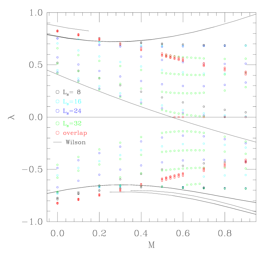
FIG. 1.: Spectral flow of the hermitian DWF operator for various $L_{s}$ and of the hermitian Wilson operator around its zero crossing on a single $8^{4}$ instanton background. Also shown is the flow of the overlap-Dirac operator which has zero eigenvalues after the crossing, setting in discontinuously.

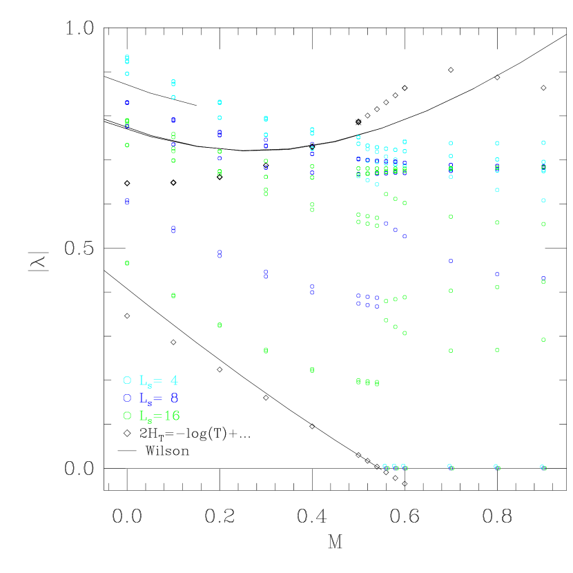
FIG. 2.: Spectral flow of the projected DWF operator, projecting the five lowest eigenvectors of $H_{T}$, for various $L_{s}$ on the same instanton background as in Fig. 1. With projection, the lowest DWF eigenvalue drops to (near) zero discontinuously after the Wilson crossing. Also shown are the flows of $H_{w}$ and $2*H_{T}$. The eigenvalues of $2*H_{T}$ track closely those of $H_{w}$.

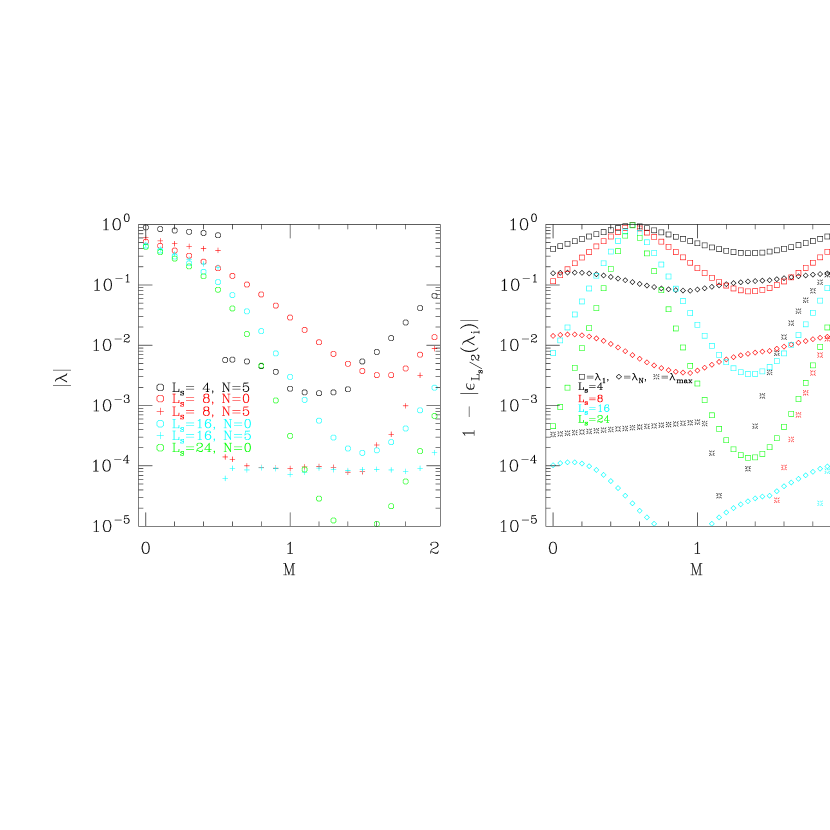
FIG. 3.: Results for DWF on the same $8^{4}$ instanton background as in in Fig. 1. The left panel shows a logarithmic plot of how the lowest (near) zero eigenvalue (with extent $L_{s}$ and $N$ eigenvectors projected) slowly rises with decreasing accuracy of the epsilon approximation as shown on the right. The right panel shows the quality of the approximation of $|\epsilon_{L_{s}/2}(\lambda_{i})|$ to unity for eigenvalues $\lambda_{i}$ of $H_{T}$. The $\lambda_{1}$ deviations shows the quality for the standard action, $\lambda_{N}$ is for the fifth eigenvalue, and $\lambda_{max}$ is for the highest eigenvalue. The smallest projected domain wall eigenvalue rises as the deviation for $\lambda_{max}$ increases.

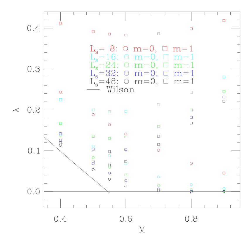
FIG. 4.: Spectral flow of the lowest pseudo-fermion eigenvalue ($m=1$) and lowest domain wall eigenvalue ($m=0$, with no projection) for various $L_{s}$ on a single $8^{4}$ instanton background. The minimum of the lowest pseudo-fermion eigenvalues is at the Wilson crossing and decreases with increasing $L_{s}$.

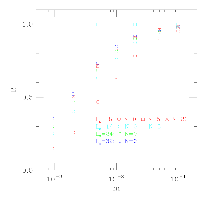
FIG. 5.: The ratio given by the Gellmann-Oakes-Renner relation (GMOR) for $M=0.5$ (just before the crossing) as a function of $L_{s}$ and projection on a single $8^{4}$ instanton background. $N$ denotes the number of projected eigenvectors. Projection for $L_{s}=16$ helps to satisfy GMOR since for all unprojected eigenvalues of $H_{T}$, $\epsilon(H_{T})$ is well approximated. For $L_{s}=8$, the deviation for the largest projected eigenvalue is still large as seen in Fig. 3.

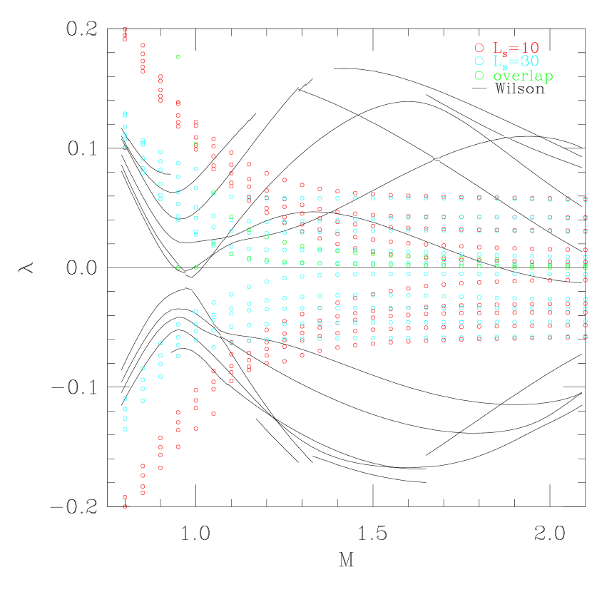
FIG. 6.: Spectral flow of the hermitian (unprojected) DWF operator for various $L_{s}$, and of the hermitian Wilson and overlap-Dirac operators on a quenched SU(3), $\beta=5.85$, $8^{3}\times 32$ configuration around the zero crossing of the Wilson flow. The overlap operator correctly finds zero eigenvalues around $M=1$ while the domain wall operator misses them.

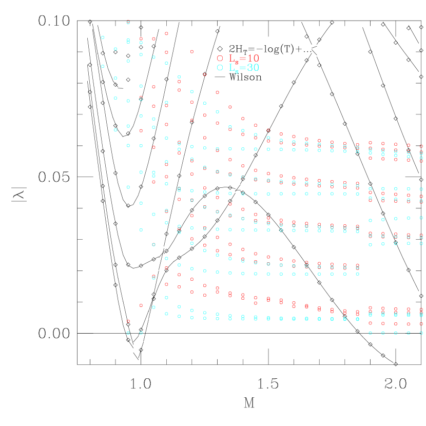
FIG. 7.: Spectral flow of the projected DWF operator, projecting the 20 lowest eigenvectors of $H_{T}$, for various $L_{s}$ on the quenched SU(3) configuration of Fig. 6. With projection, the lowest domain wall eigenvalue drops to zero (within precision used here) discontinuously after the crossing around $1.85$. The zero eigenvalues around $M=1$ are also correctly identified. Also shown are the flows of $H_{w}$ and $2*H_{T}$. The eigenvalues of $2*H_{T}$ track closely those of $H_{w}$.

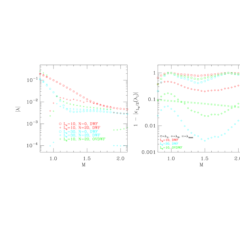
FIG. 8.: Results for the quenched SU(3) configuration of Fig. 6. The presentation is similar to Fig. 3. DWF and OVDWF are the domain wall operator and Boriçi’s variant, resp., with $N$ eigenvectors projected. The left panel shows how the lowest (near) zero eigenvalue slowly rises with decreasing accuracy of the epsilon approximation as shown on the right. The right panel shows the quality of the approximation of $|\epsilon_{L_{s}/2}(\lambda_{i})|$ for eigenvalues $\lambda_{i}$ of $H_{T}$. Here $N=20$ eigenvectors are projected. For domain wall, the 20-th eigenvalue is badly approximated for $L_{s}=8$ but slightly better for the Boriçi variant. For $L_{s}=30$, the deviation of $\lambda_{\max}$ is below the range shown.

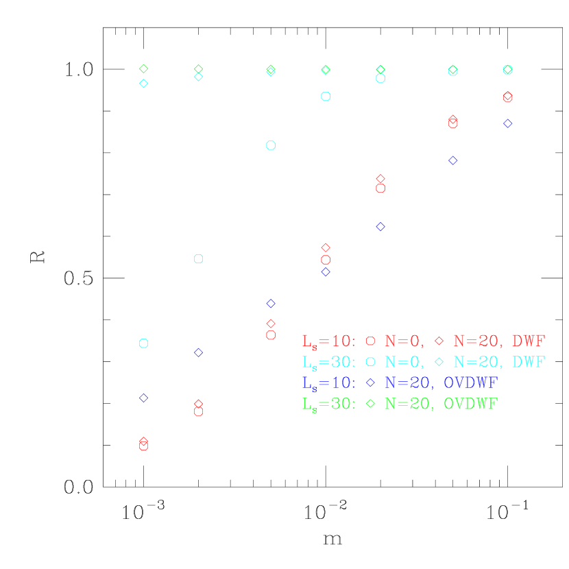
FIG. 9.: The ratio given by the Gellmann-Oakes-Renner relation (GMOR, c.f. (107)) for $M=1.65$ (just before the crossing) as a function of $L_{s}$ and projection on the same quenched SU(3) configuration as in Fig. 6. DWF and OVDWF are the domain wall operator and Boriçi’s variant, resp. For $L_{s}=30$ with projection, the GMOR relation is well satisfied but some discrepancy is seen from deviations of $H_{T}$ eigenvalues $\lambda_{i}$ in Fig. 8.

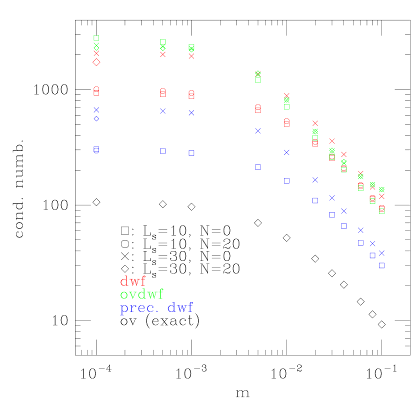
FIG. 10.: Condition numbers as a function of the mass for various actions on the same quenched SU(3) configuration and parameters as in Fig. 9. The overlap operator has the lowest condition number.

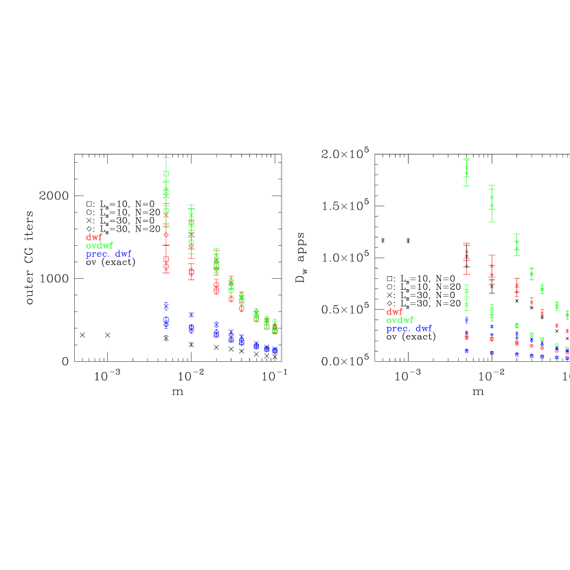
FIG. 11.: The left panel shows the number of (outer) CGNE applications to reach convergence of $10^{-5}$. The right panel shows the total number of $D_{w}$ applications for convergence (including inner and outer CG applications) on the same quenched SU(3) configuration and parameters as in Fig. 9. The overlap operator needs the fewest CG iterations. For $L_{s}=30$ with projection, the standard (un-preconditioned) domain wall and overlap operator have comparable $D_{w}$ application counts. Preconditioning saves the domain wall operator about a factor of two to three in cost.

REFERENCES

- [1] D.B. Kaplan, Phys. Lett. B288, 342 (1992).
- [2] R. Narayanan and H. Neuberger, Nucl. Phys. B443, 305 (1995).
- [3] For some recent reviews see, H. Neuberger, hep-lat/9909042, hep-lat/9910040; M. Lüscher, hep-lat/9909150.
- [4] Y. Shamir, Nucl. Phys. B406, 90 (1993).
- [5] P. Vranas, Phys. Rev. D57, 1415 (1998); S. Aoki and Y. Taniguchi, Phys. Rev. D59, 054510 (1999); Y. Kikukawa and H. Neuberger, Nucl. Phys. B526, 572 (1998).
- [6] P. Chen, N. Christ, G. Fleming, A. Kaehler, C. Malureanu, R. Mawhinney, G. Siegert, C. Sui, P. Vranas and Y. Zhestkov, hep-lat/9812011; T. Blum, Nucl. Phys. Proc. Suppl. 73, 167 (1999).
- [7] G. Fleming, hep-lat/9909140; S. Aoki, T. Izubuchi, Y. Kuramashi, and Y. Taniguchi, hep-lat/0004003.
- [8] H. Neuberger, Phys. Rev. Lett. 81, 4060 (1998).
- [9] R.G. Edwards, U.M. Heller and R. Narayanan, Nucl. Phys. B540, 457 (1999).
- [10] R.G. Edwards, U.M. Heller and R. Narayanan, Parallel Computing 25, 1395 (1999).
- [11] A. Frommer, S. Güsken, T. Lippert, B. Nöckel, K. Schilling, Int. J. Mod. Phys. C6, 627 (1995); B. Jegerlehner, hep-lat/9612014.
- [12] R.G. Edwards, U.M. Heller and R. Narayanan, Phys. Rev. D59, 094510 (1999).
- [13] R.G. Edwards, U.M. Heller and R. Narayanan, Phys. Rev. D60, 034502 (1999).
- [14] A. Boriçi, hep-lat/9909057, hep-lat/9912040.
- [15] H. Neuberger, Phys. Lett. B417, 141 (1998).
- [16] H. Neuberger, Phys. Rev. D57, 5417 (1998).
- [17] Y. Shamir, Phys Rev. D59, 054506 (1999).
- [18] T.A. DeGrand, Comp. Phys. Comm. 52, 161 (1988); T.A. DeGrand and P. Rossi, Comp. Phys. Comm. 60, 211 (1990).
- [19] R.G. Edwards, U.M. Heller and R. Narayanan, Nucl. Phys. B522, 285 (1998).
- [20] B. Bunk, K. Jansen, M. Lüscher and H. Simma, DESY-Report (September 1994); T. Kalkreuter and H. Simma, Comput. Phys. Commun. 93 (1996) 33.
- [21] P. Chen, N. Christ, G. Fleming, A. Kaehler, C. Malureanu, R. Mawhinney, G. Siegert, C. Sui, P. Vranas, Y. Zhestkov, Nucl. Phys. Proc. Suppl. 73, 207 (1999).
- [22] A. Boriçi, PhD Thesis, CSCS TR-96-27, ETH Zürich (1996).
- [23] H. Neuberger, hep-lat/9909043; R. Narayanan and H. Neuberger, in preparation.