A Lattice Study of the Glueball Spectrum^†

Abstract

Glueball spectrum is studied using an improved gluonic action on asymmetric lattices in the pure $SU(3)$ gauge theory. The smallest spatial lattice spacing is about $0.08fm$ which makes the extrapolation to the continuum limit more reliable. In particular, attention is paid to the scalar glueball mass which is known to have problems in the extrapolation. Converting our lattice results to physical units using the scale set by the static quark potential, we obtain the following results for the glueball masses: $M_{G}(0^{++})=1730(90)MeV$ for the scalar glueball mass and $M_{G}(2^{++})=2400(95)MeV$ for the tensor glueball.

PACS: 12.38.Gc, 11.15.Ha, 12.39.Mk Keywords: Glueball spectrum, Lattice QCD.

 
$\diamond$Email: chuan@mail.phy.pku.edu.cn
$\dagger$Work supported by the Chinese Natural Science Foundation under Grant No. 17500000, Pandeng fund, Startup fund from MOE and the Startup fund from Peking University.

1 Introduction

It is believed that QCD is the theory which describes strong interactions among quarks and gluons. A direct consequence of this is the existence of excitations of gluonic degrees of freedom, i.e. glueballs. However, due to their non-perturbative nature, the spectrum of glueballs can only be investigated reliably with non-purterbative methods like lattice QCD [1, 2, 3, 4]. Recently, it has become clear that such a calculation can be performed on a relatively coarse lattice using an improved gluonic action on asymmetric lattices [5, 6, 7]. In this paper, we present our results for a glueball spectrum calculation. The spatial lattice spacing in our simulations ranges from $0.08fm$ to $0.25fm$ which enables us to extrapolate more reliably to the continuum limit. The improved gluonic action we used is the tadpole improved gluonic action on asymmetric lattices as described in [6, 7]. It is given by:

$$S= - \beta\sum_{i>j}\left[{5\over 9}{TrP_{ij}\over\xi u^{4}_{s}}-{1\over 36}{TrR_{ij}\over\xi u^{6}_{s}}-{1\over 36}{TrR_{ji}\over\xi u^{6}_{s}}\right]$$ (1)

$$- \beta\sum_{i}\left[{4\over 9}{\xi TrP_{0i}\over u^{2}_{s}}-{1\over 36}{\xi TrR_{i0}\over u^{4}_{s}}\right]\;\;.$$

In the above expression, $\beta$ is related to the bare gauge coupling, $\xi=a_{s}/a_{t}$ is the (bare) aspect ratio of the asymmetric lattice with $a_{s}$ and $a_{t}$ being the lattice spacing in spatial and temporal direction respectively. The parameter $u_{s}$ is the tadpole improvement parameter to be determined self-consistently from the spatial plaquettes in the simulation. $P_{ij}$ and $P_{0i}$ are the spatial and temporal plaquette variables. $R_{ij}$ designates the $2\times 1$ Wilson loop ($2$ in direction $i$ and $1$ in direction $j$). Using spatially coarse and temporally fine lattices helps to enhance signals in the glueball correlation functions. Therefore, the bare aspect ratio is taken to be some value larger than one. In our simulation, we have used $\xi=3$ for our glueball calculation. It turns out that, using the non-perturbatively determined tadpole improvement [8] parameter $u_{s}$, the renormalization effects of the aspect ratio is small [6, 7], typically of the order of a few percent for practical values of $\beta$ in the simulation. This could also be verified by measuring corresponding Wilson loops, which will directly yield the renormalized aspect ratio. For the moment, we will ignore their difference and simply use the bare value of $\xi$. It is also noticed that, without tadpole improvement, this renormalization effect could be as large as $30$ percent [6, 7].

This paper is organized as follows. In the next section, we will explain our calculation of the Wilson loops, glueball correlation functions which give us the mass values of the glueballs in various symmetry sectors. Finite volume errors are discussed and more importantly, finite lattice spacing errors are analyzed. Special attention is paid to the scalar sector where the extrapolation used to be troublesome at coarse lattices. In the last section, we will have some discussion of out result and conclude.

2 Monte Carlo Simulations

Glueball spectrum calculations in pure gauge theory basically involve three stages. The first stage, gauge field configurations are generated using some algorithm. We have utilized a Hybrid Monte Carlo algorithm to update gauge field configurations. Several lattice sizes have been simulated and the detailed information can be found in Table.1.

Table 1: Simulation parameters and the corresponding lattice spacing in physical units obtained from Wilson loop measurements.

Lattices	$\beta$	$\lambda_{W}$	$n_{W}$	$r_{0}/a_{s}$
$8^{3}\times 24$	$2.4$	$0.20\sim 0.40$	$2\sim 4$	$1.98(2)$
$8^{3}\times 24$	$2.6$	$0.20\sim 0.40$	$2\sim 4$	$2.48(2)$
$8^{3}\times 24$	$3.0$	$0.20\sim 0.40$	$4\sim 6$	$4.11(4)$
$8^{3}\times 24$	$3.2$	$0.25\sim 0.50$	$4\sim 6$	$5.89(8)$
$10^{3}\times 30$	$3.2$	$0.25\sim 0.50$	$4\sim 6$	$5.89(8)$

For each lattice with fixed bare parameters, order of $10^{3}$ configurations have been accumulated. Each gauge field configuration is separated from the previous one by several Hybrid Monte Carlo trajectories, typically $5\sim 10$, to make sure that they are sufficiently decorrelated. Further binning of the data has been performed and no noticeable remaining autocorrelation has been observed.

The second stage of the calculation is to perform measurements of physical observables using the accumulated gauge field configurations. In fact, two independent measurements have to be done. One is to set the scale in physical units, i.e. to determine the lattice spacing $a_{s}$ in physical units. This is necessary since there is no scale in a pure gauge theory. The second is to measure glueball mass values in lattice units. This is done by measuring various glueball correlation functions. With the scale being set in the first step, the mass values of the glueballs can then be converted into physical units.

In the final stage of the calculation, glueball mass values obtained from a finite lattice have to be extrapolated to the continuum limit. This means that finite volume effects and finite lattice spacing errors have to be eliminated. Typically, finite volume errors are found to be small in these calculations [6, 7]. It is the finite lattice spacing errors that are more difficult to handle, especially for the scalar glueball mass. It was observed that, the scalar glueball sector exhibits a dip in the extrapolation, making the extrapolation less dependable compared with other channels [6]. To remedy this situation, a simulation at a smaller values of $a_{s}$ has been performed. In our calculation, we also performed a simulation at a smaller lattice spacing where $a_{s}\sim 0.08fm$. These two simulations now makes the extrapolation in the scalar sector more dependable and less sensitive to the form of the functions used in the extrapolation.

2.1 Setting the scale

In our simulation, the scale is set by measuring Wilson loops from which the static quark anti-quark potential $V(R)$ is obtained. Using the static potential between quarks, we are able to determine the lattice spacing in physical units by measuring $r_{0}$, a pure gluonic scale determined from the static potential [9]. The definition of the scale $r_{0}$ is given by: $R^{2}dV(R)/dR]_{R=r_{0}}=1.65$. In physical units, $r_{0}$ is roughly $0.5fm$ which is determined by comparison with potential models. For a recent determination of $r_{0}$, please consult Ref. [10].

In order to measure the Wilson loops accurately, it is the standard procedure to perform single link smearing [2, 6] on the spatial gauge links of the configurations. In this procedure, each spatial gauge link is replaced by a linear combination of the original link and its spatial staples. Each spatial gauge staple is weighted by a parameter $\lambda_{W}$ relative to the original gauge link. The final result is then projected back into $SU(3)$. This smearing scheme can be performed iteratively on the spatial links of gauge fields for as many as $n_{W}$ times. The effect of smearing is to projects out higher excitation contaminations from the Wilson loop measurements. Then, Wilson loops are constructed using these smeared links. For a Wilson loop of size $R\times T$, it is fitted against:

$$W(R,T)\stackrel{{\scriptstyle T\rightarrow\infty}}{{\sim}}Z(R)e^{-V(R)T}\;\;.$$ (2)

Therefore, by extracting the effective mass plateau at large temporal separation, the static quark potential $V(R)$ is obtained. We have measured the Wilson loops along different lattice axis. It is seen that the measured data points for the quark anti-quark potential along different lattice axis lie on a universal line which is an indication that the improved action restores the rotational symmetry quite well. The smearing parameter $\lambda_{W}$ used in this process are also listed in Table. 1. Using smearing, we have been able to obtain descent plateau in the effective mass and the potential $a_{t}V(R)$ is thus determined for various values of $R/a_{s}$.

The static quark potential is fitted according to a Coulomb term plus a linear confining potential which is known to work well at these lattice spacings [7]. The potential is parameterized as:

$$V(R)=V_{0}+e_{c}/R+\sigma R\;\;.$$ (3)

From this and the definition of $r_{0}$, it follows that:

$$r_{0}/a_{s}=\sqrt{{1.65+e_{c}\over\sigma a^{2}_{s}}}\;\;.$$ (4)

To convert the measured result to $r_{0}/a_{s}$, we have also used the value of $\xi$ taken as the bare value. As explained earlier, the renormalization effects for this parameter is small. The result of the spatial lattice spacing in physical units is also included in Table. 1. The errors for the ratio $r_{0}/a_{s}$ are obtained by blocking the whole data set into smaller blocks and obtain the error from different blocks.

2.2 Glueball mass measurement

To obtain glueball mass values, it is necessary to constructed glueball operators in various symmetry sectors of interests. On a lattice, the full rotational symmetry is broken down to only cubic symmetry, which is a finite point group with $5$ irreducible representations . They are labeled as : $A_{1}$, $A_{2}$, $E$, $T_{1}$ and $T_{2}$. The first two irreducible representations are one-dimensional. The third is two-dimensional while the last two are three-dimensional. In practice, one is interested in the scalar, tensor and vector glueballs in the continuum limit. The correspondence is the following: scalar glueball is in the $A_{1}$ representation of the cubic group; tensor glueball is in representation $E+T_{2}$, which forms a $5$-dimensional representation; vector glueballs are in the representation $T_{1}$. Of course, this correspondence is not one to one but infinite to one. Therefore, what we can measure is the lowest excitation in the corresponding representation of the cubic group [11, 3].

Glueball correlation functions are notoriously difficult to measure. They die out so quickly and it is very difficult to get a clear signal. In order to enhance the signal of glueball correlation functions, smearing and fuzzying have to be performed on spatial links of the gauge fields [2, 6, 7]. These techniques greatly enhance the overlap of the glueball states and thus provide possibility of measuring the mass values.

Figure 1: The Wilson loop shapes used in constructing the glueball operators.

In our simulations, after performing single link smearing and double link fuzzying on spatial links, we first construct raw operators at a given time slice $t$: $\{{\mathcal{R}}^{(i)}_{t}=\sum_{{\bf x}}{\mathcal{W}}^{(i)}_{{\bf x},t}\}$, where ${\mathcal{W}}^{(i)}_{t,{\bf x}}$ are closed Wilson loops originates from a given lattice point $x=(t,{\bf x})$. The loop-shapes studied in this calculation are shown in Fig.1. Then, elements from the cubic group is applied to these raw operators and the resulting set of loops now forms a basis for a representation of the cubic group. Suitable linear combinations of these operators are constructed to form a basis for a particular irreducible representation of interest [3]. We denote these operators as $\{{\mathcal{O}}^{(R)}_{\alpha}(t)\}$ where $R$ labels a specific irreducible representation and $\alpha$ labels different operators at a given time slice $t$. In order to maximize the overlap with one glueball state, we construct a glueball operator ${\mathcal{G}}^{(R)}(t)=\sum_{\alpha}v^{(R)}_{\alpha}\bar{{\mathcal{O}}}^{(R)}_{\alpha}(t)$, where $\bar{{\mathcal{O}}}^{(R)}_{\alpha}(t)={\mathcal{O}}^{(R)}_{\alpha}(t)-\langle 0\mid{\mathcal{O}}^{(R)}_{\alpha}(t)\mid 0\;\rangle$. The coefficients $v^{(R)}_{\alpha}$ are to be determined from a variational calculation. To do this, we construct the correlation matrix:

$${\mathbf{C}}_{\alpha\beta}(t)=\sum_{\tau}\langle 0\mid\bar{{\mathcal{O}}}^{(R)}_{\alpha}(t+\tau)\bar{{\mathcal{O}}}^{(R)}_{\alpha}(\tau)\mid 0\;\rangle\;\;.$$ (5)

The coefficients $v^{(R)}_{\alpha}$ are chosen such that they minimize the effective mass

$$m_{eff}(t_{C})=-{1\over t_{C}}\log\left[{\sum_{\alpha\beta}v^{(R)}_{\alpha}v^{(R)}_{\beta}{\mathbf{C}}_{\alpha\beta}(t_{C})\over\sum_{\alpha\beta}v^{(R)}_{\alpha}v^{(R)}_{\beta}{\mathbf{C}}_{\alpha\beta}(0)}\right]\;\;,$$ (6)

where $t_{C}$ is time separation for the optimization. In our simulation $t_{C}=1$ is taken. If we denote the optimal values of $v^{(R)}_{\alpha}$ by a column vector ${\mathbf{v}}^{(R)}$, this minimization is equivalent to the following eigenvalue problem:

$${\mathbf{C}}(t_{C})\cdot{\mathbf{v}}^{(R)}=e^{-t_{C}m_{eff}(t_{C})}{\mathbf{C}}(0)\cdot{\mathbf{v}}^{(R)}\;\;.$$ (7)

The eigenvector ${\mathbf{v}}^{(R)}_{0}$ with the lowest effective mass then yields the coefficients $v^{(R)}_{0\alpha}$ for the operator ${\mathcal{G}}^{(R)}_{0}(t)$ which best overlaps the lowest lying glueball in the channel with symmetry $R$. Higher-mass eigenvectors of this equation will then overlap predominantly with excited glueball states of a given symmetry channel.

With these techniques, the glueball mass values are obtained in

Table 2: Glueball mass estimates for the symmetry channel $A^{++}_{1}$, $E^{++}$ and $T^{++}_{2}$ at various lattice spacings. The entries corresponding to the highest $beta$ value are the values after the infinite volume extrapolation. The last row tabulated the continuum extrapolated result of the glueball mass values in units of $1/r_{0}$.

$\beta$	$a_{t}M_{A^{++}_{1}}$	$a_{t}M_{E^{++}}$	$a_{t}M_{T^{++}_{2}}$
$2.4$	$0.552(8)$	$0.980(10)$	$1.002(9)$
$2.6$	$0.482(12)$	$0.760(16)$	$0.798(15)$
$3.0$	$0.322(8)$	$0.460(13)$	$0.470(13)$
$3.2$	$0.233(7)$	$0.323(12)$	$0.340(10)$
$\infty$	$4.23(22)$	$5.77(34)$	$5.92(32)$

lattice units and the final results are listed in Table.2. The errors are obtained by binning the total data sets into several blocks and doing jackknife on the blocks.

2.3 Extrapolation to the continuum limit

As has been mentioned, finite volume errors are eliminated by performing simulations at the same lattice spacing but different physical volumes. This also helps to purge away the possible toleron states whose energy are sensitive to the size of the volume. A simulation at a larger volume is done for the smallest lattice spacing in our calculation. We found that the mass of the scalar glueball remains unchanged when the size of the volume is increased. The mass of the tensor glueball seems to be affected, which is consistent with the known result that tensor glueballs have a rather large size and therefore feel the finiteness of the volume more heavily. The infinite volume is obtained by extrapolating the finite volume results using the relation [12]:

$$a_{t}M^{(R)}(L_{s})=a_{t}M^{(R)}(\infty)\left(1-\lambda^{(R)}\exp(-\sqrt{3}z/2)/z\right)\;\;,$$ (8)

where $z=M^{(A^{++}_{1})}L_{s}$. Using the results for the mass of the $E^{++}$ and $T_{2}$ glueballs on $8^{3}24$ and $10^{3}30$ lattices for the same value of $\beta$, the final result for the mass of these glueball states are obtained. Glueball mass values for other symmetry sectors are not so sensitive to the finite volume effects. Therefore, in Table.2, only the extrapolated values for the smallest physical volume are tabulated. Other entries are obtained from $8^{3}24$ lattice results.

As for the finite lattice spacing errors, special attention is paid to the scalar glueball sector where the continuum limit extrapolation was known to have problems. Due to the simulation points at small lattice spacings, around $0.1fm$ and below, the ambiguity in this extrapolation is greatly reduced. We have tried to extrapolate the result using different formula suggested in Ref. [7], the extrapolated results are all consistent within statistical errors. For definiteness, we take the simple form:

$$r_{0}M_{G}(a_{s})=r_{0}M_{G}(0)+c_{1}(a_{s}/r_{0})^{2}+c_{2}(a_{s}/r_{0})^{4}\;\;,$$ (9)

and

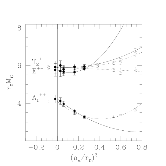
Figure 2: The continuum limit extrapolation of glueball mass values in scalar and tensor channels. The solid symbols are results from this calculation with the corresponding continuum limit extrapolation represented by the solid lines. For comparison, the corresponding results from [7] are also shown with open symbols and dashed lines.

the result is illustrated in Fig.2. The final extrapolated results for the glueball mass values are also listed in Table.2. The data points from our simulation results are shown with solid symbols and the corresponding extrapolations are plotted as solid lines. It is also noticed that the extrapolated mass values for $E^{++}$ and $T^{++}_{2}$ channels coincide within statistical errors, indicating that in the continuum limit, they form the tensor representation of the rotational group. For comparison, simulation results from [7] are also shown with open symbols and the corresponding extrapolation are represented by the dashed lines. We also tried to extrapolate linearly in $(a_{s}/r_{0})^{2}$ using three data points with smallest lattice spacing. The results are statistically consistent with the results using the extrapolation (9) within errors. It is seen that, due to data points at lattice spacings around $0.1fm$ and below, the uncertainties in the extrapolation for the glueball mass values are reduced.

Finally, to convert our simulation results on glueball masses into physical units, we use the result $r^{-1}_{0}=410MeV$. The errors for the hadronic scale $r_{0}$ is neglected. For the scalar glueball we obtain $M_{G}(0^{++})=1730(90)MeV$. For the tensor glueball mass in the continuum, we combine the results for the $T^{++}_{2}$ and $E^{++}$ channels and obtain $M_{G}(2^{++})=2400(95)MeV$ for the tensor glueball mass.

3 Discussions and Conclusions

We have studied the glueball spectrum at zero momentum in the pure $SU(3)$ gauge theory using Monte Carlo simulations on asymmetric lattices with the lattice spacing in the spatial directions ranging from $0.08fm$ to $0.25fm$. This helps to make extrapolations to the continuum limit with more confidence for the scalar and tensor glueball states. The mass values of the glueballs are converted to physical units in terms of the hadronic scale $r_{0}$. We obtain the mass for the scalar glueball and tensor glueball to be: $m_{G}(0^{++})=1730(90)MeV$ and $m_{G}(2^{++})=2400(95)MeV$. It is interesting to note that, around these two mass values, experimental glueball candidates exist. Of course, in order to compare with the experiments other issues like the mixing effects and the the effects of quenching have to be studied.

References

- [1] G. Bali et al., Phys. Lett. B 309, 378 (1993).
- [2] C. Michael and M. Teper, Nucl. Phys. B 314, 347 (1989).
- [3] B. Berg and A. Billoire, Nucl. Phys. B 221, 109 (1983).
- [4] B. Berg and A. Billoire, Nucl. Phys. B 226, 405 (1983).
- [5] M. Alford et al., Phys. Lett. B 361, 87 (1995).
- [6] C. Morningstar and M. Peardon, Phys. Rev. D 56, 4043 (1997).
- [7] C. Morningstar and M. Peardon, Phys. Rev. D 60, 034509 (1999).
- [8] G. P. Lepage and P. B. Mackenzie, Phys. Rev. D 48, 2250 (1993).
- [9] R. Sommer, Nucl. Phys. B 411, 839 (1994).
- [10] M. Guagnelli, R. Sommer, and H. Wittig, Nucl. Phys. B 535, 389 (1998).
- [11] R. C. Johnson, Phys. Lett. B 114, 147 (1982).
- [12] M. Lüscher, Commun. Math. Phys. 104, 177 (1986).