UTHEP-404 UTCCP-P-66 KANAZAWA-00-03 Domain Wall Fermions in Quenched Lattice QCD

Abstract

We study the chiral properties and the validity of perturbation theory for domain wall fermions in quenched lattice QCD at $\beta=6.0$. The explicit chiral symmetry breaking term in the axial Ward-Takahashi identity is found to be very small already at $N_{s}=10$, where $N_{s}$ is the size of the fifth dimension, and its behavior seems consistent with an exponential decay in $N_{s}$ within the limited range of $N_{s}$ we explore. From the fact that the critical quark mass, at which the pion mass vanishes as in the case of the ordinary Wilson-type fermion, exists at finite $N_{s}$, we point out that this may be a signal of the parity broken phase and investigate the possible existence of such a phase in this model at finite $N_{s}$. The $\rho$ and $\pi$ meson decay constants obtained from the four-dimensional local currents with the one-loop renormalization factor show a good agreement with those obtained from the conserved currents.

I Introduction

Domain wall fermion model[1, 2, 3] is a 5-dimensional Wilson fermion with free boundaries in the fifth dimension. At each of the boundaries either of the left- and right-handed chiral mode is expected to be localized exponentially, and hence the mixing between them, which represents the explicit chiral symmetry breaking effects, is suppressed exponentially. In the large $N_{s}$ limit, where $N_{s}$ is the size of the fifth direction, domain wall QCD (DWQCD) would have the desirable features, such as (i) no fine tuning for the chiral limit, (ii) $O(a^{2})$ scaling violation and (iii) no mixing between three- and four-quark operators with different chiralities. It is shown that these expectations are realized within the perturbation theory up to the one-loop level in the limit $N_{s}\rightarrow\infty$ [4, 5, 6, 7, 8]. Pioneering numerical studies also seem to support these expectations[9, 10].

In this paper we focus on two issues. One is the chiral properties of DWQCD at the finite $N_{s}$. It is of great importance to understand correctly how the ideal chiral properties are realized nonperturbatively as $N_{s}$ increases. We investigate the $N_{s}$ dependence of the explicit chiral symmetry breaking term in the axial Ward-Takahashi identity, which are expected to be exponentially suppressed as the $N_{s}$ increases. Correspondingly, at finite $N_{s}$, the pion remains massive in the chiral limit. We notice, however, that the pion mass at finite $N_{s}$ may vanish at some non-zero value of quark mass, which we call the critical quark mass, in a similar manner that the pion mass in the Wilson fermion formulation vanishes at the critical hopping parameter. In the case of the Wilson fermion formulation, it is well known that the massless pion implies the existence of a parity(-flavor) broken phase[11]. The analysis of two-dimensional Gross-Neveu model with domain-wall fermions indeed demonstrates the existence of the parity broken phase at the finite $N_{s}$, and the negative critical quark mass goes to zero as $N_{s}$ increases[12, 13]. In this paper we explore the negative quark mass region to examine the possible existence of the parity broken phase in the four-dimensional DWQCD.

Another important issue in this paper is the validity of the perturbation theory for DWQCD. Recently we calculated the renormalization factors for the bilinear operators[6] and three- and four-quark operators[7], for the latter of which we find the multiplicative renormalizability at infinite $N_{s}$ as opposed to the Wilson fermion case. We test the validity of the perturbation theory comparing the $\rho$ and $\pi$ meson decay constants extracted from the local currents with those from the conserved ones.

This paper is organized as follows. In Sec. II we present the details of simulation including the action of domain wall fermion. The chiral properties of DWQCD are investigated in Sec. III, where we also examine the existence of the parity broken phase. In Sec. IV we test the validity of the perturbation theory for DWQCD using the meson decay constants. Our conclusions and discussions are summarized in Sec. V.

II Details of Numerical Simulation

A Action

The domain wall fermion action is written as[2, 3]

$$S_{f} = -\sum_{x,s,y,{s^{\prime}}}{\bar{\psi}}(x,s)D_{dwf}(x,s;y,{s^{\prime}})\psi(y,{s^{\prime}})~{},$$ (1)

$$D_{dwf}(x,s;y,{s^{\prime}}) = (5-M)\delta_{x,y}\delta_{s,{s^{\prime}}}-D^{4}(x,y)\delta_{s,{s^{\prime}}}-D^{5}(s,{s^{\prime}})\delta_{x,y}~{},$$ (2)

$$D^{4}(x,y) = \frac{1}{2}\left[(1-\gamma_{\mu})U_{x,\mu}\delta_{x+\hat{\mu},y}+(1+\gamma_{\mu})U^{\dagger}_{y,\mu}\delta_{x-\hat{\mu},y}\right],$$ (3)

$$D^{5}(s,{s^{\prime}}) = \left\{\begin{array}[]{lll}P_{L}\delta_{2,{s^{\prime}}}&&(s=1)\\ P_{L}\delta_{s+1,{s^{\prime}}}&+P_{R}\delta_{s-1,{s^{\prime}}}&(1<s<N_{s})\\ &P_{R}\delta_{N_{s}-1,{s^{\prime}}}&(s=N_{s})\end{array}\right.$$ (7)

with domain wall height $M$ and the extent of the fifth dimension $N_{s}$. The right- and left-handed projection operators are defined by $P_{R,L}=(1\pm\gamma_{5})/2$. The chiral zero mode is supposed to appear for $M>0$. The index $x,y$ stands for four-dimensional lattice sites, while the index $s,{s^{\prime}}$ for the fifth direction runs from 1 to $N_{s}$.

The quark fields on the four-dimensional space-time are given by combinations of the fermion fields at the boundaries,

$$q(x)=P_{L}\psi(x,1)+P_{R}\psi(x,N_{s})~{},$$ (8)

$$\bar{q}(x)=\bar{\psi}(x,1)P_{R}+\bar{\psi}(x,N_{s})P_{L}~{},$$ (9)

where the left(right) chiral zero mode is well localized at $s=1(N_{s})$ for $0<M<2$ in the free theory.

The explicit bare quark mass $m_{f}$ is introduced as

$$S_{f}\rightarrow S_{f}-\sum_{x}m_{f}\bar{q}(x)q(x)~{},$$ (10)

which provides the quarks in eqs.(8) and (9) with a Dirac mass ${\bar{m}_{f}}$. For the free quark case, we obtain ${\bar{m}_{f}}=M(2-M)m_{f}$ in the $N_{s}\longrightarrow\infty$ limit[2].

The action (1) is invariant under global SU($N_{f}$) symmetry, which yields the five-dimensional conserved current[3],

$$j^{a}_{\mu}(x,s) = \frac{1}{2}\left[{\bar{\psi}}(x,s)(-1+\gamma_{\mu})U_{x,\mu}\frac{\lambda^{a}}{2}\psi(x+{\hat{\mu}},s)+{\bar{\psi}}(x+{\hat{\mu}},s)(1+\gamma_{\mu})U^{\dagger}_{x,\mu}\frac{\lambda^{a}}{2}\psi(x,s)\right],$$ (11)

where $\lambda^{a}/2$ $(a=1,\dots,N_{f}^{2}-1)$ are generators of SU($N_{f}$) group. In terms of this current we can define the conserved vector and axial currents,

$$V_{\mu}^{a,{\rm con}}(x) = \sum_{s=1}^{N_{s}}j_{\mu}^{a}(x,s),$$ (12)

$$A_{\mu}^{a,{\rm con}}(x) = -\sum_{s=1}^{N_{s}}{\rm sign}\left(\frac{N_{s}}{2}-s+\frac{1}{2}\right)j_{\mu}^{a}(x,s).$$ (13)

We should note that $A_{\mu}^{a,{\rm con}}$ is not exactly conserved in the finite $N_{s}$ contrary to the vector case: the divergence of $A_{\mu}^{a,{\rm con}}$ satisfies

$$\left\langle\nabla_{\mu}^{-}A_{\mu}^{a,{\rm con}}(x){\cal O}(y)\right\rangle=2m_{f}\left\langle{\bar{q}}(x)\gamma_{5}\frac{\lambda^{a}}{2}q(x){\cal O}(y)\right\rangle+2\left\langle J^{a}_{5q}(x){\cal O}(y)\right\rangle$$ (14)

with

$$J^{a}_{5q}(x)=-{\bar{\psi}}(x,N_{s}/2)P_{L}\frac{\lambda^{a}}{2}\psi(x,N_{s}/2+1)+{\bar{\psi}}(x,N_{s}/2+1)P_{R}\frac{\lambda^{a}}{2}\psi(x,N_{s}/2),$$ (15)

where $\nabla_{\mu}^{-}$ is the backward difference operator: $\nabla_{\mu}^{-}f(x)=f(x)-f(x-\mu)$ and ${\cal O}$ is some operator. We will set $x\neq y$ in our numerical simulation. The contribution of $J^{a}_{5q}(x)$ in eq.(14) is expected to be exponentially suppressed as the $N_{s}$ increases for the physical operator ${\cal O}_{\rm phys.}(\bar{q},q)$.

B Simulation parameters

The simulation is carried out with the plaquette gauge action at $\beta=6.0$ on $16^{3}\times 32\times N_{s}$ lattices in quenched QCD. Table I summarizes our run parameters. We generated gauge configurations on a $16^{3}\times 32$ lattice with the five-hit pseudo heat-bath algorithm. Each configuration is separated by 2000 sweeps after 20000 sweeps for the initial thermalization. In DWQCD the same gauge configuration is assigned on each layer of the fifth direction. The $\rho$ meson mass at the chiral limit ($m_{f}=0$) is used to determine the lattice spacing, which gives $a^{-1}\sim 2$GeV with $m_{\rho}=770$MeV as input while slightly depending on $M$ and $N_{s}$ (see Sec. III). The mean-field estimate for the optimal value of $M$ gives[4]

$$M=1+4(1-u)=1.819~{},$$ (16)

employing $u=1/(8K_{c})$ with $K_{c}=0.1572$ for the Wilson fermion at $\beta=6.0$.

The quark propagator is obtained by solving the inverse of the quark matrix (2) with the unit wall source without gauge fixing,

$$\sum_{y,{s^{\prime}}}\sum_{b}D^{ab}_{dwf}(x,s;y,{s^{\prime}})G^{b}_{\psi}(y,{s^{\prime}})=B^{a}(x,s)~{},$$ (17)

$$~{}~{}~{}~{}B^{a}(x,s)={1\over 3V_{s}}\sum_{c}\delta_{ac}\delta_{t,0}\sum_{\vec{x}^{\prime}}\delta_{{\vec{x}},{\vec{x}^{\prime}}}\left[\delta_{s,1}P_{R}+\delta_{s,N_{s}}P_{L}\right]~{},$$ (18)

where $x=({\vec{x}},t)$ with spatial coordinates $\vec{x}$ and time coordinate $t$; $V_{s}$ is the spatial volume and $a,b,c$ denote the color indices. The four-dimensional quark propagator is constructed with a linear combination of $G_{\psi}$,

$$G_{q}(x)=P_{L}G_{\psi}(x,1)+P_{R}G_{\psi}(x,N_{s})~{}.$$ (19)

To solve the linear equation (17), we employ the conjugate gradient method with even/odd preconditioning[14]. In the case of $m_{f}=0.025$, about 500 iterations are needed to satisfy a convergence criterion which requires $|r|^{2}/|G_{\psi}|^{2}<10^{-12}$ with the residual $r$. Neither minimal residue(MR) nor BiCGStab converges within a practical number of iterations for gauge configurations at $\beta\sim 6.0$. Throughout this paper, statistical errors are estimated by the single elimination jackknife method.

III Chiral properties of DWQCD

A Restoration of chiral symmetry

We investigate the existence of the chiral zero mode expected in the limit of $m_{f}\to 0$ and $N_{s}\to\infty$ using the pion mass at the chiral limit ($m_{f}=0$) and the anomalous contribution $J_{5q}$ in the PCAC relation (14). The pion mass $m_{\pi}(m_{f},N_{s},M)$ is extracted from a global fit of the two-point function

$$\sum_{{\vec{x}},{\vec{y}}}\left\langle J_{\pi}({\vec{x}},t)J_{\pi}^{\dagger}({\vec{y}},0)\right\rangle$$ (20)

employing the fitting function

$$V_{s}\frac{|\left\langle 0|J_{\pi}|\pi\right\rangle|^{2}}{2m_{\pi}}\left({\rm e}^{-m_{\pi}t}+{\rm e}^{-m_{\pi}(32-t)}\right),$$ (21)

where $J_{\pi}(x)={\bar{q}}(x)\gamma_{5}q(x)$. We choose the fitting range to be $9\leq t\leq 23$ after taking account of the time reversal symmetry $t\rightarrow 32-t$.

Figure 1 shows the $m_{f}a$ dependence of $m_{\pi}^{2}$. We observe a good linear behavior for the pion mass squared as a function of $m_{f}$. Employing a linear extrapolation, we obtain the value of $m_{\pi}^{2}$ at $m_{f}=0$, which is shown in Fig. 2 as a function of $M$. We find that the minimum point of the pion mass is around $M=1.819$, which shows the mean-field estimation of optimal $M$ in (16) is reasonably accurate. Furthermore, extending the linear extrapolation into the negative $m_{f}$ region, as is done for the ordinary Wilson-type fermion, we can also extract the critical quark mass $m_{c}(N_{s},M)$ at which the pion mass squared vanishes. As we expected, both $m_{\pi}^{2}$ at $m_{f}=0$ and $m_{c}(N_{s},M)$ decreases monotonically as $N_{s}$ increases. In Fig. 3 we plot $m_{\pi}^{2}$ for $m_{f}a=$0.075, 0.050, 0.025 and 0 as a function of $N_{s}$, where $m_{\pi}^{2}(m_{f}=0)$ is the extrapolated value. The magnitude of $m_{\pi}^{2}$ at $m_{f}=0$ seems to diminish exponentially in $N_{s}$. In order to confirm that $m_{\pi}^{2}$ at $m_{f}=0$ indeed vanishes exponentially in $N_{s}$, one has to further increase $N_{s}$. However, we do not attempt such an investigation at the present lattice size, since $m_{\pi}^{2}(m_{f}=0)$ at $N_{s}=10$ is already as small as that for the Nambu-Goldstone pion of the Kogut-Susskind fermion, which gives an estimate of the finite size effect to the would-be massless pion at the same $\beta$ and the spatial lattice size.

It is reported, at $\beta=6.0$ on a $16^{3}\times 32$ lattice, that $m_{\pi}^{2}=0.014(2)$ in the chiral limit for $N_{s}=16$ and $M=1.8$[15], which is roughly equal to our value of $m_{\pi}^{2}=0.0093(54)$ for $N_{s}=10$ and $M=1.819$.

The anomalous contribution due to $J_{5q}$ in eq.(14) is evaluated by calculating the ratio of two-point functions,

$$\frac{\sum_{{\vec{x}},{\vec{y}}}\left\langle J_{5q}({\vec{x}},t)J_{\pi}^{\dagger}({\vec{y}},0)\right\rangle}{\sum_{{\vec{x}},{\vec{y}}}\left\langle J_{\pi}({\vec{x}},t)J_{\pi}^{\dagger}({\vec{y}},0)\right\rangle}\stackrel{{\scriptstyle t\gg 0}}{{\longrightarrow}}\frac{\left\langle 0|J_{5q}|\pi\right\rangle}{\left\langle 0|J_{\pi}|\pi\right\rangle},$$ (22)

where we employ a constant fit over the range $8\leq t\leq 24$. This quantity measures contribution of the explicit chiral symmetry breaking effects in the PCAC relation:

$$\frac{\left\langle 0|2J_{5q}|\pi\right\rangle}{\left\langle 0|J_{\pi}|\pi\right\rangle}=\frac{\left\langle 0|\nabla_{\mu}^{-}A_{\mu}^{\rm con}|\pi\right\rangle}{\left\langle 0|J_{\pi}|\pi\right\rangle}-2m_{f}.$$ (23)

In Fig. 4 we plot the results for ${\left\langle 0|J_{5q}|\pi\right\rangle}/{\left\langle 0|J_{\pi}|\pi\right\rangle}$ as a function of $m_{f}a$. The data shows little $m_{f}$ dependence at each $N_{s}$. We obtain the value of ${\left\langle 0|J_{5q}|\pi\right\rangle}/{\left\langle 0|J_{\pi}|\pi\right\rangle}$ at $m_{f}=0$ by extrapolating the data linearly to $m_{f}=0$. Figure 5 illustrates the $N_{s}$ dependence of ${\left\langle 0|J_{5q}|\pi\right\rangle}/{\left\langle 0|J_{\pi}|\pi\right\rangle}$ at $m_{f}a=$0.075, 0.050, 0.025, 0, where we also plot the results for $|m_{c}|$ for comparison. We find that the magnitude of ${\left\langle 0|J_{5q}|\pi\right\rangle}/{\left\langle 0|J_{\pi}|\pi\right\rangle}$ decreases exponentially as $N_{s}$ increases. The same situation is observed for $|m_{c}|$. These features suggest that the chiral symmetry would be restored in the limit of $m_{f}\to 0$ and $N_{s}\to\infty$ at $\beta=6.0$.

Note that $|m_{c}|$ and ${\left\langle 0|J_{5q}|\pi\right\rangle}/{\left\langle 0|J_{\pi}|\pi\right\rangle}$ are expected to be consistent, if the latter has no $m_{f}$ dependence as seen in Fig. 4. However we observe a slight deviation between them in Fig. 5. We point out two possibilities to yield this inconsistency. One is the finite size effects on the pion mass and the other is the quenched chiral logarithm plaguing the pion mass in the quenched approximation. We should note that the quantity ${\left\langle 0|J_{5q}|\pi\right\rangle}/{\left\langle 0|J_{\pi}|\pi\right\rangle}$ is free from both systematic contaminations, which assures that ${\left\langle 0|J_{5q}|\pi\right\rangle}/{\left\langle 0|J_{\pi}|\pi\right\rangle}$ is superior to $|m_{c}|$ to measure the remnant of the chiral symmetry breaking effects in DWQCD.

We briefly mention the determination of the lattice spacing $a$ from the $\rho$ meson mass. Figure 6 shows the $N_{s}$ dependence of $m_{\rho}a$ at $m_{f}=0$ (circles) and at $m_{f}=m_{c}$ (squares) with $M=1.819$, which are obtained by a linear extrapolation from the data. For small $N_{s}(=4)$, $m_{\rho}a$ at $m_{f}=0$ differs from the one at $m_{f}=m_{c}$ beyond statistical errors, while the difference almost vanishes at $N_{s}=10$. This is true for other values of $M$: within statistical errors the values of $m_{\rho}a$ at $m_{f}=0$ and $m_{f}=m_{c}$ are consistent with each other for $M=1.7-1.9$ at $N_{s}=10$. Furthermore the $M$ dependence of $m_{\rho}$ itself is mild over this range of $M$ at $N_{s}=10$. ¿From the value of $m_{\rho}a$ at $m_{f}=0$ with $M=1.819$ and $N_{s}=10$, we estimate $a^{-1}=2.02(17)$GeV from $m_{\rho}=770$MeV as an input.

B Parity broken phase

In the Wilson fermion formalism, the critical quark mass is identified with the second order phase transition point between the (spontaneously) parity broken phase and the parity symmetric phase[11]. The massless pion is understood as the massless particle associated with the second order phase transition. Recently, the study of the two-dimensional Gross-Neveu model with domain wall fermions pointed out that this picture is true even for this model at finite $N_{s}$[12, 13]. In this section we examine whether the massless pion at $m_{f}=m_{c}$ at finite $N_{s}$ can be understood in this way.

For the finite $N_{s}$, the parity broken phase may exist in negative $m_{f}$ regions. From the study of the two-dimensional Gross-Neveu model with domain wall fermions[13], we expect the phase diagram in Fig. 7 for four-dimensional DWQCD. Each of five critical points, where the $m_{\pi}^{2}=0$ line is touched on $g^{2}=0$ line at $m_{f}=-(1-M+2l)^{N_{s}}$ ($l=0,1,2,3,4$), corresponds to the massless particle pole of momentum

$$p_{\mu}(l=0) = (0,0,0,0),$$ (24)

$$p_{\mu}(l=1) = (\frac{\pi}{a},0,0,0),(0,\frac{\pi}{a},0,0),(0,0,\frac{\pi}{a},0),(0,0,0,\frac{\pi}{a}),$$ (25)

$$p_{\mu}(l=2) = (\frac{\pi}{a},\frac{\pi}{a},0,0),(\frac{\pi}{a},0,\frac{\pi}{a},0),(\frac{\pi}{a},0,0,\frac{\pi}{a})$$ (27)

$$,(0,\frac{\pi}{a},\frac{\pi}{a},0),(0,\frac{\pi}{a},0,\frac{\pi}{a}),(0,0,\frac{\pi}{a},\frac{\pi}{a})$$

$$p_{\mu}(l=3) = (\frac{\pi}{a},\frac{\pi}{a},\frac{\pi}{a},0),(\frac{\pi}{a},\frac{\pi}{a},0,\frac{\pi}{a}),(\frac{\pi}{a},0,\frac{\pi}{a},\frac{\pi}{a}),(0,\frac{\pi}{a},\frac{\pi}{a},\frac{\pi}{a}),$$ (28)

$$p_{\mu}(l=4) = (\frac{\pi}{a},\frac{\pi}{a},\frac{\pi}{a},\frac{\pi}{a}).$$ (29)

Since the critical point for the $p_{\mu}(l=0)$ mode converges to $m_{f}=0$ for $0<M<2$ as $N_{s}$ increases, while other four critical points move rapidly to $|m_{f}|=\infty$, we can expect one small ($|m_{f}|<1$) critical point and four large ($|m_{f}|>1$) critical points at finite $N_{s}$ in four-dimensional DWQCD.

Based on these speculation, let us investigate existence of the “cusp”(branch) corresponding the $p_{\mu}(l=0)$ mode, which provides an evidence of the parity broken phase. We calculate pion masses at $m_{f}a=-0.120,-0.100,-0.093,-0.086,-0.080$ for $N_{s}=4$ and $M=1.819$. Without adding the external field which couples to the parity broken order parameter, one can not perform the correct simulation in the parity broken phase. To avoid the direct simulation in the parity broken phase, we take rather large magnitudes for negative $m_{f}$ values so that the system goes into another symmetric phase, and try to find another side of the phase boundary (critical quark mass) from this phase. In Fig. 8 we plotted the $\pi$ meson mass squared $m_{\pi}^{2}$ as a function of $m_{f}$. Extrapolations of $m_{\pi}^{2}$ to zero both from positive and negative $m_{f}$, where four largest $m_{f}$ are used for negative $m_{f}$, indicate that a parity broken phase may exist around $m_{f}a\sim-0.03$. We can interpret that Fig. 8 represents the portion in Fig. 7 denoted by dashed segment. It is noted that the large errors for negative $m_{f}$ are caused by the fact that the pion propagators form peculiar shapes similar to “W” character, which has been often observed near the another side of the parity broken phase for the Wilson fermion[16].

IV Meson decay constants

A Perturbative renormalization factors

The $\rho$ meson decay constant $f_{\rho}$ is defined by

$$\left\langle 0|V_{\mu}|\rho\right\rangle=\epsilon_{\mu}m_{\rho}^{2}/f_{\rho}~{},$$ (30)

where $m_{\rho}$ is the $\rho$ meson mass and $\epsilon_{\mu}$ is the polarization vector. We have two choices for the vector current $V_{\mu}$: the exactly conserved current in eq.(12) and the four-dimensional local current $V_{\mu}^{q}(x)={\bar{q}}(x)\gamma_{\mu}q(x)$ multiplied by the renormalization factor $Z_{V}$.

In a similar way, the $\pi$ meson decay constant $f_{\pi}$ is given by

$$\left\langle 0|A_{\mu}|\pi\right\rangle=p_{\mu}f_{\pi}~{},$$ (31)

where $p_{\mu}$ denotes the momentum of the pion and $A_{\mu}$ is either the (almost) conserved current in eq.(13) or the four-dimensional local current $A_{\mu}^{q}(x)={\bar{q}}(x)\gamma_{\mu}\gamma_{5}q(x)$ multiplied by the renormalization factor $Z_{A}$.

Perturbative technique in DWQCD is already applied to evaluation of the renormalization factors for the bilinear operators[6] and three- and four-quark operators[7] consisting of four-dimensional quarks in eqs.(8) and (9). It is shown that $Z_{S}=Z_{P}=Z_{m}^{-1}$ and $Z_{V}=Z_{A}$ at $N_{s}\rightarrow\infty$ for the bilinear operators, which is expected in the case that the chiral Ward-Takahashi identities hold exactly[6]. Another desirable feature is that the three- and four-quark operators at $N_{s}\longrightarrow\infty$ can be renormalized without mixing between operators with different chiralities, as opposed to the Wilson fermion case[7]. The peculiar feature in the renormalization of DWQCD, however, is an appearance of the overlap factor $(1-|1-M|^{2})Z_{w}$ for the four-dimensional quark fields. The one-loop coefficient $z_{w}$ of $Z_{w}$ in (34) is of $O(10-10^{2})$ for $|1-M|\hbox to0.0pt{\lower 3.5pt\hbox{$\mathchar 0\relax\sim$}\hss}\raise 1.0pt\hbox{$>$}0.1$ without mean-field improvement, which could be problematic because the present simulation is done for $M\geq 1.7$. It is shown in Ref.[6], however, that the magnitude of the one-loop coefficient for $Z_{w}$ is reduced to $O(1)$ for $|1-{\tilde{M}}|\hbox to0.0pt{\lower 3.5pt\hbox{$\mathchar 0\relax\sim$}\hss}\raise 1.0pt\hbox{$>$}0.1$ after the mean field replacement from $M$ to ${\tilde{M}}=M+4(u-1)$. Therefore, comparing the $\rho$($\pi$) meson decay constant $f_{\rho}$($f_{\pi}$) obtained from $Z_{V}V_{\mu}^{q}$($Z_{A}A_{\mu}^{q}=Z_{V}A_{\mu}^{q}$) with that from $V_{\mu}^{\rm con}$($A_{\mu}^{\rm con}$) gives a good testing ground for the validity of the (mean field improved) perturbation theory.

Following the notation of Ref.[6], the renormalization factor of $V_{\mu}^{q}$ is written as

$$V_{\mu}^{\rm con}=\frac{1}{(1-w_{0}(M)^{2})Z_{w}(M)}Z_{V}(M)V_{\mu}^{q},$$ (32)

where

$$w_{0}(M) = 1-M,$$ (33)

$$Z_{w}(M) = 1+\frac{g^{2}}{16\pi^{2}}C_{F}z_{w}(M),$$ (34)

$$Z_{V}(M) = 1+\frac{g^{2}}{16\pi^{2}}C_{F}z_{V}(M),$$ (35)

without mean-field improvement. $C_{F}=(N^{2}-1)/(2N)$ is the quadratic Casimir in SU($N$) gauge group. In the case of $M=1.819$, we find $1-w_{0}^{2}=0.32924$, $z_{w}(M)=250.36$ and $z_{V}(M)=-17.760$ using the results in Ref.[6]. The large corrections of $1/(1-w_{0}^{2})$ and $Z_{w}$ could jeopardize the efficiency of the perturbation theory. However, once a mean-field improvement is employed, the renormalization factors are reexpressed as

$$V_{\mu}^{\rm con}=\frac{1}{(1-w_{0}({\tilde{M}})^{2})Z_{w}^{{\rm MF}}({\tilde{M}})}uZ_{V}^{{\rm MF}}({\tilde{M}})V_{\mu}^{q}$$ (36)

with

$${\tilde{M}} = M+4(u-1),$$ (37)

$$w_{0}({\tilde{M}}) = 1-{\tilde{M}},$$ (38)

$$Z_{w}^{\rm MF}({\tilde{M}}) = 1+\frac{g^{2}}{16\pi^{2}}C_{F}z_{w}^{\rm MF}({\tilde{M}}),$$ (39)

$$Z_{V}^{\rm MF}({\tilde{M}}) = 1+\frac{g^{2}}{16\pi^{2}}C_{F}z_{V}^{\rm MF}({\tilde{M}}).$$ (40)

With the use of $u=0.87781=\sqrt[4]{P}$, where $P$ is the expectation value of the plaquette, we obtain ${\tilde{M}}=1.3302$, $1-w_{0}({\tilde{M}})^{2}=0.89095$, $z_{w}^{\rm MF}(\tilde{M})=7.327$ and $z_{V}^{\rm MF}(\tilde{M})=-7.3744$ from the results in Ref.[6, 7]. It is remarkable that the perturbative corrections are drastically reduced. We determine the coupling constant at the scale $1/a$ in the ${\overline{\rm MS}}$ scheme with the aid of the mean-field improvement,

$$\frac{1}{g^{2}_{\overline{\rm MS}}(1/a)}=P\frac{\beta}{6}-0.13486.$$ (41)

Incorporating ${g^{2}_{\overline{\rm MS}}(1/a)}$ in eqs.(39) and (40), we finally obtain the value of the renormalization factor with the mean-field improvement,

$$\frac{1}{(1-w_{0}({\tilde{M}})^{2})Z_{w}^{{\rm MF}}({\tilde{M}})}uZ_{V}^{{\rm MF}}({\tilde{M}})=0.7504.$$ (42)

If we employ $u=1/(8K_{c})$ with $K_{c}=0.1572$ for the mean field improvement, we obtain $0.7147$ instead of $0.7504$ in eq.(42). Since their difference is smaller than the statistical errors of the $\rho$ and $\pi$ meson decay constants, we use the value of eq.(42) for the renormalization factor in the next subsection.

B $\rho$ and $\pi$ meson decay constants

We calculate $f_{\rho}$ from the ratio of two point functions,

$$\frac{\sum_{{\vec{x}},{\vec{y}}}\left\langle V_{\mu}^{{\rm con},q}({\vec{x}},t)J_{\rho}^{\dagger}({\vec{y}},0)\right\rangle}{\sum_{{\vec{x}},{\vec{y}}}\left\langle J_{\rho}({\vec{x}},t)J_{\rho}^{\dagger}({\vec{y}},0)\right\rangle}\left\langle 0|J_{\rho}|\rho\right\rangle\stackrel{{\scriptstyle t\gg 0}}{{\longrightarrow}}\left\langle 0|V_{\mu}^{{\rm con},q}|\rho\right\rangle,$$ (43)

where $J_{\rho}(x)={\bar{q}}(x)\gamma_{i}q(x)$ $(i=1,2,3)$ is the interpolating field for the $\rho$ meson. The amplitude $\left\langle 0|J_{\rho}|\rho\right\rangle$ is obtained by fitting the two-point function with

$$\sum_{{\vec{x}},{\vec{y}}}\left\langle J_{\rho}({\vec{x}},t)J_{\rho}^{\dagger}({\vec{y}},0)\right\rangle=V_{s}\frac{|\left\langle 0|J_{\rho}|\rho\right\rangle|^{2}}{2m_{\rho}}\left({\rm e}^{-m_{\rho}t}+{\rm e}^{-m_{\rho}(32-t)}\right),$$ (44)

where the fitting range is chosen to be $8\leq t\leq 24$.

In Fig.9 we plot the $\rho$ meson decay constants obtained from $V_{\mu}^{q}$ and $V_{\mu}^{\rm con}$ as a function of $m_{f}$. We observe that both results are consistent once the perturbative corrections are applied to $V_{\mu}^{q}$. This is an encouraging evidence to show the validity of the perturbation theory with the mean-field improvement. Still, the scaling violation effects should be checked. The value at the chiral limit $m_{f}=0$, which is obtained by extrapolating the results for the conserved current linearly, is found to be slightly smaller than the experimental value.

Let us turn to the $\pi$ meson decay constant $f_{\pi}$. We obtain $f_{\pi}$ from correlation functions of the axial vector current $A_{\mu}(x)$ and the interpolating field for the $\pi$ meson $J_{\pi}(x)={\bar{q}}(x)\gamma_{5}q(x)$,

$$\sum_{{\vec{x}},{\vec{y}}}\left\langle X({\vec{x}},t)Y^{\dagger}({\vec{y}},0)\right\rangle=V_{s}\frac{\left\langle 0|X|\pi\right\rangle\left\langle\pi|Y^{\dagger}|0\right\rangle}{2m_{\pi}}\left({\rm e}^{-m_{\pi}t}+{\rm e}^{-m_{\pi}(32-t)}\right),$$ (45)

where $X,Y=J_{\pi},A_{4}$. The fitting range is chosen to be $9\leq t\leq 23$.

Figure 10 shows a comparison of the $\pi$ meson decay constants obtained from $A_{4}^{q}$ and $A_{4}^{\rm con}$. We find the same situation as in the case of the $\rho$ meson decay constant: the perturbative corrections sufficiently compensate the difference between $A_{4}^{q}$ and $A_{4}^{\rm con}$. Linear extrapolation of the results for the conserved current gives the value at the chiral limit $m_{f}=0$, which is roughly consistent with the experimental value. We also show the $M$ dependence of $f_{\pi}$ at $m_{f}=0$ in Fig. 11. Although the results slightly depend on the choice of $M$, the differences are smaller than current statistical errors.

V Conclusions and discussions

We have investigated the chiral properties of DWQCD by measuring the pion mass and the explicit chiral symmetry breaking term in the PCAC relation. Their $N_{s}$ dependence up to $N_{s}=10$ seem to be consistent with exponential decay in $N_{s}$, which indicates that the chiral symmetry is restored at $N_{s}\to\infty$ limit, as expected. More extensive study with larger $N_{s}$, however, is required to confirm this conclusion.

We also calculate the pion mass at negative $m_{f}$ to examine whether there exists the parity broken phase in DWQCD. Our result is consistent with the existence of the parity broken phase.

The validity of the perturbation theory in DWQCD is tested by calculating the $\rho$ and $\pi$ meson decay constants from the four-dimensional local currents and the conserved ones. We find that the difference between both currents is sufficiently compensated with the perturbative renormalization factor up to the one-loop level with the aid of the mean-field improvement. This is an encouraging result, though the magnitude of the scaling violation on these quantities should be checked further.

FIG. 1.: Pion mass squared as a function of $m_{f}a$ at $M=1.819$ and $N_{s}=4,6,10$. Solid lines show linear fits.

FIG. 2.: Pion mass squared extrapolated to $m_{f}\to 0$ as a function of $M$ at $N_{s}=4,6,10$.

FIG. 3.: Pion mass squared as a function of $N_{s}$ at $M=1.819$. Filled square shows the value for the Nambu-Goldstone pion of the Kogut-Susskind fermion at $\beta=6.0$ on a $16^{3}\times 40$ lattice.

FIG. 4.: ${\left\langle 0|J_{5q}|\pi\right\rangle}/{\left\langle 0|J_{\pi}|\pi\right\rangle}$ extrapolated as a function of $m_{f}a$ at $M=1.819$ with $N_{s}=4,6,8$. Solid lines show linear fits.

FIG. 5.: ${\left\langle 0|J_{5q}|\pi\right\rangle}/{\left\langle 0|J_{\pi}|\pi\right\rangle}$ as a function of $N_{s}$ at $M=1.819$ for $m_{f}a=0.075,0.050,0.025,0$ together with the critical quark mass $|m_{c}|$.

FIG. 6.: $\rho$ meson mass extrapolated to $m_{f}=0$ and $m_{f}=m_{c}$ as a function of $N_{s}$ at $M=1.819$ .

FIG. 7.: Schematic phase diagram in ($g^{2},m_{f}$) plane for $N_{s}=$even. See text for dashed segment.

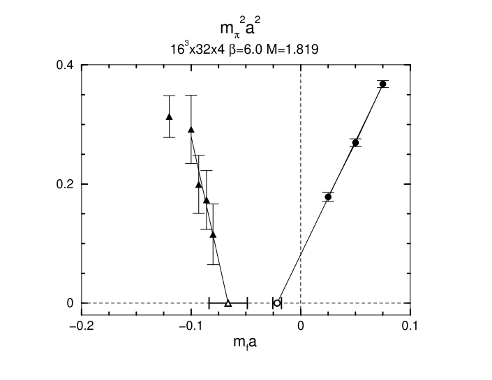
FIG. 8.: $m_{\pi}^{2}$ in lattice unit as a function of $m_{f}a$ at $M=1.819$ and $N_{s}=4$. Solid lines show linear extrapolations.

FIG. 9.: $f_{\rho}$ as a function of $m_{f}a$ at $M=1.819$ and $N_{s}=10$ together with the experimental value. Data points for $Z_{V}V_{\mu}^{q}$ (filled squares) are slightly displaced horizontally for clarity. Solid line shows linear extrapolation of the results for the conserved current.

FIG. 10.: $f_{\pi}$ in lattice unit as a function of $m_{f}a$ at $M=1.819$ and $N_{s}=10$ together with the experimental value. Data points for $Z_{A}A_{\mu}^{q}$ (filled squares) are slightly displaced horizontally for clarity. Solid line shows linear extrapolation of the results for the conserved current.

FIG. 11.: $f_{\pi}$ in lattice unit extrapolated to $m_{f}a\to 0$ as a function of $M$ at $N_{s}=10$ together with the experimental value.

TABLE I.: Simulation parameters on $16^{3}\times 32\times N_{s}$ lattices in the quenched QCD.

$N_{s}$	$4$	$6$	$10$
No. conf.	$20$	$10$	$30(M=1.819),20$
$M$	$1.7$	$1.819$	$1.7$
	$1.75$		$1.819$
	$1.819$		$1.9$
	$1.85$
	$1.9$
	$1.95$
	$2.0$
$m_{f}a$	$0.075$	$0.075$	$0.075$
	$0.050$	$0.050$	$0.050$
	$0.025$	$0.025$	$0.025$
	$-0.08\;(M=1.819)$
	$-0.086\;(M=1.819)$
	$-0.093\;(M=1.819)$
	$-0.10\;(M=1.819)$
	$-0.12\;(M=1.819)$

REFERENCES

• [1] D. B. Kaplan, Phys. Lett. B288 (1992) 342.
• [2] Y. Shamir, Nucl. Phys. B406 (1993) 90.
• [3] V. Furman and Y. Shamir, Nucl. Phys. B439 (1995) 54.
• [4] S. Aoki and Y. Taniguchi, Phys. Rev. D59 (1999) 054510.
• [5] S. Aoki and Y. Taniguchi, Phys. Rev. D59 (1999) 094506.
• [6] S. Aoki, T. Izubuchi, Y. Kuramashi and Y. Taniguchi, Phys. Rev. D59 (1999) 094505.
• [7] S. Aoki, T. Izubuchi, Y. Kuramashi and Y. Taniguchi, Phys. Rev. D60 (1999) 114504.
• [8] J. Noaki and Y. Taniguchi, hep-lat/9906030 (to appear in Physical Review D).
• [9] T. Blum and A. Soni, Phys. Rev. D56 (1997) 174; Phys. Rev. Lett. 79 (1997) 3595.
• [10] For a review, see T. Blum, Nucl. Phys. B (Proc. Suppl.) 73 (1999) 167.
• [11] S. Aoki, Phys. Rev. D30 (1984) 2653; Phys. Rev. Lett. 57 (1986) 3136; Nucl. Phys. B314 (1989) 79.
• [12] P. Vranas, I. Tziligakis and J. Kogut, hep-lat/9905018.
• [13] T. Izubuchi and K. Nagai, hep-lat/9906017.
• [14] T. A. DeGrand, Comput. Phys. Commun. 52 (1988) 161; T. A. DeGrand and P. Rossi, Comput. Phys. Commun. 60 (1990) 211.
• [15] L. Wu, hep-lat/9909117.
• [16] S. Aoki, T. Kaneda and A. Ukawa, Phys. Rev. D56 (1997) 1808.
Refer to caption