HU-EP-00/17 WUB 00-06 HLRZ 2000-4
Static potentials and glueball masses from QCD simulations with Wilson sea quarks

Abstract

We calculate glueball and torelon masses as well as the lowest lying hybrid potential in addition to the static ground state potential in lattice simulations of QCD with two flavours of dynamical Wilson fermions. The results are obtained on lattices with $16^{3}\times 32$ and $24^{3}\times 40$ sites at $\beta=5.6$, corresponding to a lattice spacing, $a^{-1}=2.65^{+5}_{-8}$ GeV, as determined from the Sommer force radius, at physical sea quark mass. The range spanned in the present study of five different quark masses is reflected in the ratios, $0.83\geq m_{\pi}/m_{\rho}\geq 0.57$.

I Introduction

The expectation that gluons form bound states, so-called glueballs, is as old as QCD itself [1]. Indeed, such states make up the spectrum of pure $SU(3)$ gauge theory and have rather precisely been determined in quenched lattice simulations [2, 3, 4]. However, an unambiguous experimental confirmation of their existence is still missing. Lattice simulations have provided an explanation for this situation: most of the glueballs come out to be quite heavy [2, 4] and will therefore manifest themselves as very broad resonances with many decay channels. This holds in particular for the most interesting glueballs, those with spin-exotic, i.e. quark model forbidden, quantum numbers.

However, a conservative interpretation of results obtained in the valence quark (or quenched) approximation to QCD urges us to expect (see e.g. Ref. [5]) a predominantly gluonic bound state with scalar quantum numbers, $J^{PC}=0^{++}$, and mass between 1.4 GeV and 1.8 GeV. Indeed, in this region more scalar resonances have been established experimentally than a standard quark model classification would suggest [6]. When switching on light quark flavours the difference between a glueball that contains sea quarks and a flavour singlet (isoscalar) meson that contains “glue”, sharing the same quantum numbers, becomes ill defined. In general such hypothetical, pure states will mix with each other to yield the observed hadron spectrum. This situation is different from that of flavour non-singlet hadrons which, if we ignore weak interactions, have a well defined valence quark content. Such “standard” hadrons might become unstable but otherwise retain most of their qualitative properties when sea quarks are included. Indeed ratios between masses of light standard hadrons, calculated within the quenched approximation, have been found to differ by less than about [7] 10 % from (full QCD) experiment.

One can utilise quenched lattice data on the scalar glueball and isoscalar $s\bar{s}$ as well as $u\bar{u}+d\bar{d}$ mesons as an input into phenomenologically motivated mixing models [8]. However, such models can only provide a crude scenario for the actual situation that will be clarified once the entire spectrum of full QCD has been calculated. A first attempt in this direction has been made by the HEMCGC Collaboration a decade ago [9] and recently first results from the UKQCD Collaboration on flavour singlet scalar meson/glueball masses in QCD with two light sea quark flavours have been reported [10].

At present the main target of simulations involving sea quarks is to pin down differences with respect to the quenched approximation and to develop the methodology required when a decrease of sea quark masses below $m_{\pi}/m_{\rho}\approx 0.5$ will become possible with the advent of the next generation of supercomputers. One would expect sea quarks not only to be important for glueball-meson mixing and for an understanding of the spectrum of isoscalars but for flavour singlet phenomenology in general [11, 12].

The potential between static colour sources at a separation, $r$, is one of the most precisely determined quantities in quenched lattice studies [13, 14, 15]. Two physical phenomena are expected to occur when including sea quarks, one at large and the other at small distances. The former effect is known as “string breaking” (see Ref. [16] and references therein): once $r$ exceeds a critical value, creation of a light quark-antiquark pair out of the vacuum becomes energetically preferable and the QCD “string” will break; the static-static state will decay into a pair of static-light mesonic bound states, resulting in the complete screening of colour charges at large distances that is observed in nature. The potential will approach a constant value at infinite $r$. On the other hand, the presence of sea quarks slows down the “running” of the QCD coupling as a function of the scale with respect to the quenched approximation: when running the coupling from an infra-red hadronic reference scale down to short distances, the effective Coulomb coupling in presence of sea quarks should, therefore, remain stronger than in the quenched case.

Exploratory studies [17, 18] of the zero temperature static potential with dynamical fermions focussed on the question of string breaking. However, no statistically significant signal of colour screening has been detected. A difference between the potentials with and without sea quarks at short distances has then been reported by the SESAM Collaboration in Refs. [19, 20, 21]. Later studies by the UKQCD, CP-PACS and MILC collaborations qualitatively confirm these findings [22, 23, 24], employing different lattice actions and, in the latter case, a different number of flavours.

In this paper we present a combined analysis of SESAM and T$\chi$L [25] data (as obtained on $16^{3}\times 32$ and $24^{3}\times 40$ lattices, respectively) on the static potential, torelon and glueball masses. Moreover, for the first time, we have determined the $\Pi_{u}$ hybrid potential [26] in a simulation including dynamical sea quarks. Preliminary versions of the results presented here have been published in Refs. [19, 27, 28, 20, 21, 16, 29, 5].

The article is organised as follows: in Sect. II we summarise simulation details and our parameter values and describe the measurement techniques applied. In Sect. III we discuss how the glueball and torelon masses and the potentials are determined. We also present the quality of the ground state overlaps achieved and the forms of the respective creation operators that were found to be most suitable. Subsequently, we present our physical results on the potentials, torelons and glueballs in Sect. IV, before we conclude.

II Lattice technology

We analyse samples of configurations that have been generated by means of the hybrid Monte Carlo (HMC) algorithm using the Wilson fermionic and gluonic actions with $n_{f}=2$ mass degenerate quark flavours at the inverse lattice coupling, $\beta=5.6$. This is done on $L_{\sigma}^{3}L_{\tau}=16^{3}32$ as well as on $24^{3}40$ lattices at the mass parameter values, $\kappa=0.156,0.1565,0.157,0.1575$ and 0.158. The corresponding chiralities can be quantified in terms of the ratios [30], $m_{\pi}/m_{\rho}=0.834(3),0.813(9),0.763(6),0.704(5)$ and 0.574(13), respectively. The simulation parameters are displayed in Tab. I, where the Sommer scale [31], $r_{0}\approx 0.5$ fm, is defined through the static potential, $V(r)$,

$$r^{2}\left.\frac{dV}{dr}\right|_{r=r_{0}}=1.65.$$ (1)

At each $\kappa$ value 4,000–5,000 thermalised HMC trajectories have been generated. Great care has been spent [32, 33] on investigating autocorrelations between successive HMC trajectories for the topological charge as well as for other quantities including smeared Wilson loops and Polyakov lines, similar to those used in the present study. The operators that enter the glueball and torelon analysis have been separated by two (eight at $\kappa=0.1565$, five at $\kappa=0.157$) HMC trajectories; smeared Wilson loops that are required for the potential calculations have been determined every 20 (16 at $\kappa=0.1565$) trajectories. The numbers of thermalised configurations analysed in total are denoted by $n_{\mbox{glue}}$ and $n_{\mbox{pot}}$ in the Table for the two classes of measurements, respectively.

In order to reduce statistical noise we had to employ measurement frequencies that are larger than the inverse integrated autocorrelation times in most cases. This is particularly true for the glueballs and torelons. Autocorrelation effects have been taken care of by binning the time series into blocks prior to the statistical analysis. The bin sizes have been increased until the statistical errors of the fitted parameters stabilised. The numbers of effectively independent configurations that, after this averaging process, finally entered the analysis are denoted by $m_{\mbox{glue}}$ and $m_{\mbox{pot}}$, respectively.

In addition to the dynamical quark simulations, quenched reference potential measurements have been performed. For this purpose, smeared Wilson loop data generated at $\beta=6.0$ and $\beta=6.2$ in the context of the study of Ref. [34] have been re-analysed. The hybrid $\Pi_{u}$ potential reference data have been obtained in Ref. [35] at the same two $\beta$ values.

TABLE I.: Simulation parameters. The last two rows refer to quenched simulations.

$\kappa$	$L_{\sigma}^{3}L_{\tau}$	$r_{0}a^{-1}$	$m_{\pi}aL_{\sigma}$	$n_{\mbox{glue}}$	$m_{\mbox{glue}}$	$n_{\mbox{pot}}$	$m_{\mbox{pot}}$
0.1560	$16^{3}32$	5.11(3)	7.14(4)	2128	266	236	236
0.1565	$16^{3}32$	5.28(5)	6.39(6)	500	250	322	161
0.1570	$16^{3}32$	5.48(7)	5.51(4)	1000	200	250	125
0.1575	$16^{3}32$	5.96(8)	4.50(5)	2272	142	270	90
0.1575	$24^{3}40$	5.89(3)	6.65(6)	1980	110	201	67
0.1580	$24^{3}40$	6.23(6)	4.77(7)	1780	89	196	49
$\beta=6.0$	$16^{3}32$	5.33(3)	—	—	—	570	570
$\beta=6.2$	$32^{4}$	7.29(4)	—	—	—	116	116

In order to determine glueball masses, temporal correlation functions between linear combinations of Wilson loops have been constructed. For simplicity we restricted ourselves to plaquette-like operators that can be built from four (fat) links. Torelons, i.e. flux loops that live on the torus and encircle a periodic spatial boundary [36], have been created from linear combinations of smeared spatial Polyakov (or Wilson) lines. Both, the fat plaquettes, used to construct the glueballs, and the Wilson lines can have three orthogonal spatial orientations. The real part of the sum over these orientations transforms according to the $A_{1}^{++}$ representation [37] of the relevant cubic point group, $O_{h}\otimes Z_{2}$. In order to project out the $T_{1}^{+-}$ representation one can take the imaginary part of one of the three possible orientations; the $E^{++}$ representation can be achieved by taking the real part, either of the sum of two orientations minus twice the third one or of the difference between two orientations. In order to increase statistics we average over the correlation functions obtained from the three equivalent orthogonal $T_{1}^{+-}$ or two $E^{++}$ realisations. Within all three channels, $A_{1}^{++}$, $E^{++}$ and $T_{1}^{+-}$, we subtract the disconnected parts from the correlation functions. This is only necessary for the $A_{1}^{++}$ state that carries the vacuum quantum numbers. However, in doing this for all channels, we find (slightly) reduced statistical fluctuations.

All operators are projected onto zero momentum at source and sink by averaging over all spatial sites. In the case of glueballs, the $A_{1}^{++}$, $E^{++}$ and $T_{1}^{+-}$ representations can be subduced from the continuum $O(3)\otimes Z_{2}$, $J^{PC}=0^{++},2^{++}$ and $1^{+-}$ representations, respectively, while the cubic point group remains the relevant symmetry group for the torelons (that only exist on a torus), even in the continuum limit. In what follows we shall label glueballs by the above continuum $J^{PC}$ quantum numbers.

The fat links that form the basis of the glueball and torelon creation operators have been constructed by alternating “APE smearing” [38] (keeping the length of the smeared link constant) with “Teper fuzzing” [39] (increasing the length by a factor two). In both algorithms a link of smearing level $i+1$ is formed by taking a linear combination of its predecessor of iteration $i$ (in the case of fuzzing the product of two straight $i$ level links) and the four closest surrounding spatial staples, followed by a projection back into the gauge group [13]. We denote the un-smeared links by $i=0$. The first iteration then consists of APE smearing with the relative weight of the straight line connection with respect to the staple sum being $\alpha=0$. This is followed by a fuzzing iteration with $\alpha=1.3$, APE smearing with $\alpha=0$ and so forth. This procedure is the outcome of a semi-systematic study of different fuzzing algorithms [27]. Fat links of levels 0 and 1 have effective length $a$, levels 2 and 3 length $2a$, levels 4 and 5 length $4a$ and levels 6 and 7 length $8a$. Iterations 8 and 9, yielding fat links of extent $16a$, are only performed on the $24^{3}$ lattices.

APE smearing has also been applied to obtain ground state and excited state potentials. In this case, we iterate the procedure 26 times with a straight line coefficient, $\alpha=2.3$. Subsequently, Wilson loops are constructed whose spatial parts are built from smeared links. In addition to on-axis distances, ${\mathbf{r}}\parallel(1,0,0)$, off-axis separations that are multiples of $(1,1,0)$, $(1,1,1)$, $(2,1,0)$, $(2,1,1)$ and $(2,2,1)$ have been realised for the ground state potential. In the case of the hybrid potential, in addition to on-axis separations, the plane-diagonal direction, ${\mathbf{r}}\parallel(1,1,0)$, has been investigated. The spatial gauge transporter along the latter direction is obtained by calculating the difference between the positively and negatively oriented “one-corner” paths connecting the two end points. For on-axis separations the potential in the continuum $\Pi_{u}$ representation can be obtained from the $E_{u}$ representation of $D_{4h}$. The $E_{u}$ creation operator has been constructed in the usual way [40] from the sum of two differences between forwards and backwards oriented staples. The orthogonal depth of these staples has been chosen to be one lattice unit for $r=a$, two lattice units for $2a\leq r\leq 5a$ and three lattice units for $r\geq 6a$.

III Mass determinations

A cross correlation matrix between the eight (ten in the case of the $L_{\sigma}=24$ glueballs) basis operators corresponding to different smearing/fuzzing levels is formed for each temporal separation, $t$. For the sake of numerical stability we restrict our analysis to two by two subsets of the correlation matrix, $M(t)$, with blocking level $i\geq 2$. We then select the subset of two states for which the combination, $M^{-1/2}(a)M(2a)M^{-1/2}(a)$, yields the lowest energy eigenvalue, and trace the $t$ dependence of the effective mass,

$$m_{\mbox{eff}}(t)=a^{-1}\ln\frac{C(t)}{C(t+a)},$$ (2)

calculated from the correlation function, $C(t)$, that is associated with the optimal eigenvector, in order to identify a plateau. The glueball and torelon masses are subsequently determined by means of a fully correlated and bootstrapped fit to the plateau region. The required covariance matrices are determined by means of sub-bootstraps.

We denote the state that is created by an operator of fuzzing level $i=0,1,\ldots$ within each glueball channel by $|i\rangle$. In Tabs. II and III the state vectors used to extract the $0^{++}$ and $2^{++}$ glueballs are listed, respectively, as well as the fitted overlaps of these states with the physical ground states. We have employed the normalisation, $\langle i|i\rangle=1$. The data at $\kappa=0.1565$ is less precise due to the smaller ensemble size, $n_{\mbox{glue}}$. In general, our variational procedure yields ground state overlaps around 80 %.

While a direct determination of glueball radii turns out to be impossible within our limited statistical ensemble sizes, the shapes of the optimal creation operators are indicative for the approximate diameters of the underlying physical ground states. Note that the only direct measurement of glueball sizes to-date has been attempted in pure $SU(2)$ gauge theoryin Ref. [41]. On all $16^{3}$ volumes we find the $0^{++}$ wave function to receive a dominant $|5\rangle$ component, which is one APE iteration applied to a fuzzed link of effective length $4a$. The subleading contribution is $|6\rangle$, i.e. a square with side length $8a$. We conclude that the “diameter” of the scalar glueball is somewhat less than 8 lattice spacings or 0.7 fm. These observations indicate a somewhat wider glueball than observed in previous quenched studies [42, 43, 41, 2].

As one increases $\kappa$, the effective lattice spacing, determined for instance in units of the gluonic observable, $r_{0}$, decreases and the glueball extends over more lattice sites. This results in an increased relative weight of the larger, $|6\rangle$, state, which finally becomes the dominant contribution at $\kappa=0.158$. There is a difference between the two volumes at $\kappa=0.1575$: the size of the glueball on the larger lattice becomes smaller, indicating finite size effects. As we shall see below this goes along with an increase of its mass.

The $2^{++}$ state is dominated by the $|6\rangle$ contribution, with the exception of $\kappa=0.1565$. At this $\kappa$ value the statistics are not really sufficient for a reliable determination of the optimal state vector, as indicated by the large relative error on the ground state overlap, $0.48\pm 0.20$. The second largest contribution then comes from the $|4\rangle$ ($|3\rangle$ for the $\kappa=0.1575$, $L_{\sigma}=24$ simulation) state. In general, we find the $|4\rangle$ state to have best overlap with the $1^{+-}$ glueball.

TABLE II.: Scalar glueball wave function and overlap with the physical ground state.

$\kappa$	$L_{\sigma}$	state vector	g.s. overlap
0.1560	$16$	$0.76|5\rangle+0.65|6\rangle$	0.89(2)
0.1565	$16$	$0.77|5\rangle+0.63|6\rangle$	0.71(12)
0.1570	$16$	$0.72|5\rangle+0.70|6\rangle$	0.79(4)
0.1575	$16$	$0.73|5\rangle+0.68|6\rangle$	0.83(5)
0.1575	$24$	$0.72|4\rangle+0.70|5\rangle$	0.94(9)
0.1580	$24$	$0.65|5\rangle+0.76|6\rangle$	0.80(8)

FIG. 1.: Effective scalar and tensor glueball masses and fits at $\kappa=0.156$.

FIG. 2.: Same as Fig. 1 for $\kappa=0.1565$.

TABLE III.: Tensor glueball wave function and overlap with the physical ground state.

$\kappa$	$L_{\sigma}$	state vector	g.s. overlap
0.1560	$16$	$0.37|4\rangle+0.93|6\rangle$	0.81(3)
0.1565	$16$	$0.83|4\rangle+0.55|6\rangle$	0.48(20)
0.1570	$16$	$0.28|4\rangle+0.96|6\rangle$	0.81(3)
0.1575	$16$	$0.27|4\rangle+0.96|6\rangle$	0.80(3)
0.1575	$24$	$0.37|3\rangle+0.93|6\rangle$	0.62(17)
0.1580	$24$	$0.66|4\rangle+0.75|6\rangle$	0.84(4)

FIG. 3.: Same as Fig. 1 for $\kappa=0.157$.

FIG. 4.: Same as Fig. 1 for the $16^{3}$ volume at $\kappa=0.1575$.

TABLE IV.: Torelon ground state overlaps.

$\kappa$	$L_{\sigma}$	$A_{1}^{++}$	$E^{++}$	$T_{1}^{+-}$
0.1560	16	0.89(2)	0.90(2)	0.91(2)
0.1570	16	0.87(6)	0.82(4)	0.72(11)
0.1575	16	0.41(10)	0.74(2)	0.39(12)
0.1575	24	0.55(13)	0.84(3)	0.60(21)
0.1580	24	0.85(24)	0.83(11)	0.24(9)

In Figs. 1 – 6, we show effective mass plots for the scalar and tensor glueballs at the various parameter values, together with the corresponding fit results (solid lines with dashed error bands). Plateaus could be identified either from $t=2a$ or $t=3a$ onwards. Since we take correlations between the data points into account fitted results can turn out to lie somewhat below the central values of the individual effective masses (cf. Figs. 4 and 5). The torelon masses have been analysed in an analogous way. All torelons receive their dominant contribution either from the $|6\rangle$ or $|7\rangle$ channels with a subleading term from the $|4\rangle$ or $|5\rangle$ states. The achieved ground state overlaps are listed in Tab. IV. The statistical quality of the signal did not permit an estimation of the overlap at $\kappa=0.1565$.

FIG. 5.: Same as Fig. 1 for the $24^{3}$ volume at $\kappa=0.1575$.

FIG. 6.: Same as Fig. 1 for $\kappa=0.158$.

On volumes of similar physical size in terms of $r_{0}$ we find statistical errors of fuzzed plaquettes and Wilson lines to be smaller than in comparable quenched simulations [42, 2]. This can very well be due to the larger number of degrees of freedom when including quarks. Similar conclusions can be drawn from a comparison between published $SU(2)$ and $SU(3)$ results. In the case of the determination of the static potential absolute errors on smeared Wilson loops are smaller than in comparable quenched simulations too. However, this effect is partly compensated for by a faster decay of the signal in Euclidean time, due to an increase of the static source self energy. In most gluonic quantities self-averaging over more lattice points when increasing the physical volume reduces the statistical noise. This is of course not the case for torelons that become heavier with growing volume. However, statistical fluctuations of glueball correlation functions grow with the volume too. This effect, that has also been observed in quenched simulations [42, 2], is related to contributions stemming from large distance correlators to the spatial sum that is required to project onto zero momentum.

In the potential measurements no variational optimisation is performed. Again, effective masses are traced against $t$, separately for all lattice separations, ${\mathbf{r}}$. In view of the fact that, given the exponential increase of relative errors with $t$, the result of a fit to data at $t\geq t_{\min}$ will be almost identical to the effective mass calculated at $t=t_{\min}$, we decided to estimate the potential by the latter. We also demanded the effective mass at $t_{\min}-a$ to be compatible with the quoted result, determined at $t=t_{\min}$.

FIG. 7.: Effective masses for the potential on the $24^{3}$ lattice at $\kappa=0.1575$ at four different source separations.

In Fig. 7, we illustrate the convergence of effective masses,

$$V({\mathbf{r}},t)=a^{-1}\ln\frac{W({\mathbf{r}},t)}{W({\mathbf{r}},t+a)}\longrightarrow V({\mathbf{r}})\quad(t\rightarrow\infty),$$ (3)

towards the asymptotic value, $V({\mathbf{r}})$, for the case of the $\kappa=0.1575$ potential on the $24^{3}$ volume at four randomly selected distances. Note that, due to the positivity of the Wilson action, the approach towards the plateau has to be monotonous. At $\beta=5.6$, with the smearing algorithm used, the range of $\kappa$ values investigated and the selection criterium employed, we found $V[{\mathbf{r}},t_{\min}({\mathbf{r}})]$ to approximate the asymptotic value within statistical errors for $4a\leq t_{\min}\leq 6a$, i.e. at $t_{\min}\approx r_{0}$. In the case of the $\Pi_{u}$ potentials, the ground state overlaps were found to be somewhat inferior and the statistical errors larger. As a consequence of these two competing effects the necessary $t$-cuts came out to be almost identical to those employed for the ground state potential.

For distances bigger than about $2\,r_{0}$, $t_{\min}$ had to be increased by one lattice unit with respect to its value at smaller distances. This differs from our experience from quenched studies employing similar methods at similar lattice spacings where systematic and statistical effects happened to interfere in such a way that the same $t$-cut could be applied at all distances [13, 14]. Once the potential is extracted, the overlap of the creation operator with the physical ground state can be quantified in terms of an overlap coefficient, $0<C_{0}({\mathbf{r}})\leq 1$:

$$C_{0}({\mathbf{r}},t)=W({\mathbf{r}},t)e^{V({\mathbf{r}},t)t}\longrightarrow C_{0}({\mathbf{r}})\quad(t\rightarrow\infty).$$ (4)

FIG. 8.: Ground state overlaps of the potential creation operators as a function of $r$. The quenched results have been obtained at $\beta=6.2$.

In Fig. 8, we compare the ground state overlaps that have been achieved at $\kappa=0.156$ and $\kappa=0.1575$ ($L_{\sigma}=24$) with quenched $\beta=6.2$ data that have been obtained by use of the same smearing algorithm and analysis procedure. We note that while at small $r$ the ground state overlaps of the un-quenched simulations are superior to the quenched reference data, at large $r$ the projection onto the physical ground state becomes increasingly worse, in particular at the lighter quark mass.

The dependence of the quenched overlaps on $r$ is linear to first approximation, however, this is not so for the sea quark data (which explains why $t_{\min}$ had to be increased as a function of $r$ in the latter case). We conclude that at large $r$ the flux tube distribution appears to change when including sea quarks. This effect, which becomes more pronounced when the quark mass is decreased, can be interpreted as a first indication of string breaking: the physical ground state will be a mixture between a would-be static-static state and a pair of two static-light mesons. While our creation operator is tuned to optimally project onto the former it has almost zero overlap with a wave function of the latter type. As a consequence, we lose local mass plateaus altogether in the regime, $r>2.5\,r_{0}$. A similar reduction of ground state overlaps at large distances has been reported by the CP-PACS Collaboration [44].

IV Results

A The static potentials

The potentials obtained from the six dynamical fermion and two quenched simulations have been rescaled in units of $r_{0}$. Subsequently, the constant $r_{0}V(r_{0})$ has been subtracted in all cases to cancel the (different) static self energy contributions and to achieve the common normalisation, $V(r_{0})=0$. Up to violations of rotational symmetry at small distances, the un-quenched potentials are found to agree with each other within statistical errors. In particular, we do not see finite size effects among the two $\kappa=0.1575$ data sets.

In Fig. 9, we compare the potential obtained on the largest lattice volume at our disposal, $L_{\sigma}a=24\,a\approx 4.07\,r_{0}\approx 2.03$ fm at $\kappa=0.1575$, with the quenched potential at $\beta=6.2$. Besides the ground state potentials, which correspond to the $\Sigma_{g}^{+}$ representation of the relevant continuum symmetry group $D_{\infty h}$, the $\Pi_{u}$ hybrid potentials [40, 5] are depicted as well as the approximate masses of pairs of static-light scalar and pseudoscalar bound states into which the static-static string states are expected to decay at large $r$. Note that for separations, $r>1.9\,r_{0}$, we have used some extra off-axis directions, in addition to those mentioned in Sect. II. Around $r\approx 2.3\,r_{0}$ we expect both, $\Sigma_{g}^{+}$ and $\Pi_{u}$ potentials to exhibit colour screening. However, the Wilson loop data are not yet precise enough to resolve this effect. In a forthcoming paper [45] we therefore intend to present a more systematic analysis geared to improve the statistical quality of potential data in the interesting regime, $r>2\,r_{0}$, along with a study of the corresponding transition matrix elements that might shed more light onto this question [46, 47].

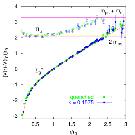
FIG. 9.: Comparison between quenched ($\beta=6.2$) and un-quenched ground state and $\Pi_{u}$ potentials.

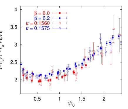
FIG. 10.: First hybrid excitation: quenched vs. un-quenched.

In Fig. 10, we compare our two most precise un-quenched data sets ($\kappa=0.156$ and $\kappa=0.1575$) on the hybrid potential with quenched results. We find no statistically significant differences, other than finite $a$ effects between the quenched potentials obtained at two different $\beta$ values (full symbols).

The ground state potentials are fitted to the parametrisation,

$$V({\mathbf{r}})=V_{0}+\sigma\,r-\frac{e}{r}+g\left(\frac{1}{r}-\left[\frac{1}{\mathbf{r}}\right]\right),$$ (5)

where the term $[1/{\mathbf{r}}]$, that denotes the tree level lattice propagator in position space [5], is included to quantify the short distance lattice artefacts. Given the fact that the number of elements in the covariance matrix is much bigger than the sizes of our data samples, we refrain from attempting correlated fits. Therefore, $\chi^{2}$ can in principle become much smaller than the degrees of freedom, $N_{DF}$. All errors are bootstrapped.

We wish to investigate the effect of sea quarks onto the short range interquark potential. Apart from the fit parameters, we also calculate the Sommer scale of Eq. (1),

$$r_{0}=\sqrt{\frac{1.65-e}{\sigma}}.$$ (6)

The fit function, Eq. (5), is only thought to effectively parameterise the potential within a given distance regime, rather than being theoretically sound. For instance neither string breaking nor the running of the QCD coupling has been incorporated. Therefore, the values of the effective fit parameters will in general depend on the fit range, $[r_{\min},r_{\max}]$. For instance, as a consequence of asymptotic freedom, $e$ will weaken as data points from smaller and smaller distances are included. To exclude such a systematic bias from our comparison between quenched and un-quenched fit parameters, we deviate somewhat from our first analysis [19] (as we have already done in Refs. [20, 21]) and use the same $r_{\min}>0.4\,r_{0}$ in physical units for all our fits and $r_{\max}<aL_{\sigma}/2$. The results are displayed in Tab. V.

Three-parameter fits have been performed in addition, by constraining $g=0$ in Eq. (5). To obtain acceptable fit qualities for the same physical fit range on all data sets we had to increase, $r_{\min}\approx 0.6\,r_{0}$. The latter fit results are shown in Tab. VI.

TABLE V.: Four-parameter fits to the static potential for $r_{\min}>0.4\,r_{0}$.

$\kappa$	$L_{\sigma}$	$\frac{r_{\min}}{a}$	$\frac{\chi^{2}}{N_{DF}}$	$g$	$V_{0}a$	$e$	$\sqrt{\sigma}a$
0.1560	16	$\sqrt{5}$	$0.94$	0.27(5)	0.731(06)	0.338(09)	0.224(2)
0.1565	16	$\sqrt{5}$	$0.54$	0.42(7)	0.738(10)	0.349(16)	0.216(3)
0.1570	16	$\sqrt{5}$	$0.78$	0.34(7)	0.725(12)	0.324(19)	0.210(4)
0.1575	16	$\sqrt{6}$	$0.47$	0.30(9)	0.739(11)	0.337(20)	0.192(4)
0.1575	24	$\sqrt{6}$	$0.76$	0.30(6)	0.746(05)	0.352(09)	0.193(2)
0.1580	24	$2\sqrt{2}$	$0.64$	0.28(7)	0.751(07)	0.358(12)	0.182(3)
$\kappa_{ph}$	—	—	—	—	0.760(12)	$0.368^{+20}_{-26}$	$0.171^{+6}_{-3}$
$\beta=6.0$	16	$\sqrt{5}$	$0.14$	0.34(2)	0.658(04)	0.291(05)	0.219(2)
$\beta=6.2$	32	$3$	$0.49$	0.25(1)	0.636(03)	0.292(05)	0.160(1)

In Tab. VII, we display the $r_{0}$ values obtained from our four-parameter interpolations as well as the effective string tension in units of $r_{0}$. The same data is depicted in Fig. 11 as a function of the squared $\pi$ mass, $(m_{\pi}a)^{2}$. Chiral extrapolations are performed according to,

$$a\,r_{0}^{-1}(m_{\pi})=a\,r_{0}^{-1}(0)+c_{1}a^{2}\,m_{\pi}^{2}+c_{2}a^{4}\,m_{\pi}^{4}.$$ (7)

The fit to all data points, with the exception of the $L_{\sigma}=16$ result at $\kappa=0.1575$, yields the parameter values,

$$a\,r_{0}^{-1}(0) = 0.1476(30),$$ (8)

$$c_{1} = 0.324(57),$$ (9)

$$c_{2} = -0.41(22),$$ (10)

$$\chi^{2}/N_{DF} = 1.37/2.$$ (11)

When excluding the rightmost point ($\kappa=0.156$) a linear extrapolation becomes possible:

$$a\,r_{0}^{-1}(0) = 0.1509(14),$$ (12)

$$c_{1} = 0.246(16),$$ (13)

$$\chi^{2}/N_{DF} = 1.32/2.$$ (14)

The fitted curves as well as the quadratically extrapolated $r_{0}^{-1}(0)$ value (open square), with error bars enlarged to incorporate the one $\sigma$ region around the linear extrapolation, are included in the Figure.

TABLE VI.: Three-parameter fits to the static potential for $r_{\min}\approx 0.6\,r_{0}$.

$\kappa$	$L_{\sigma}$	$\frac{r_{\min}}{a}$	$\frac{\chi^{2}}{N_{DF}}$	$V_{0}a$	$e$	$\sqrt{\sigma}a$
0.1560	16	$3$	$0.84$	0.712(12)	0.290(23)	0.228(3)
0.1565	16	3	$0.48$	0.715(21)	0.291(42)	0.221(6)
0.1570	16	$3$	$1.43$	0.725(21)	0.326(42)	0.210(6)
0.1575	16	$3$	$0.57$	0.727(19)	0.308(38)	0.195(5)
0.1575	24	$3$	$0.75$	0.736(07)	0.322(15)	0.195(2)
0.1580	24	$3$	$0.77$	0.747(08)	0.348(17)	0.183(3)
$\beta=6.0$	16	$3$	$0.87$	0.639(06)	0.245(19)	0.223(3)
$\beta=6.2$	32	$3\sqrt{2}$	$0.67$	0.637(05)	0.296(13)	0.160(1)

TABLE VII.: $r_{0}$ and the ratio $\sqrt{\sigma}r_{0}$.

$\kappa$	$L_{\sigma}$	$r_{0}/a$	$\sqrt{\sigma}r_{0}$
0.1560	16	5.104(29)	1.145(4)
0.1565	16	5.283(52)	1.141(7)
0.1570	16	5.475(72)	1.152(8)
0.1575	16	5.959(77)	1.146(9)
0.1575	24	5.892(27)	1.139(4)
0.1580	24	6.230(60)	1.137(5)
$\kappa_{ph}$	—	$6.73^{+13}_{-19}$	$1.133_{-8}^{+11}$
$\beta=6.0$	16	5.328(31)	1.166(2)
$\beta=6.2$	32	7.290(34)	1.165(2)

FIG. 11.: Chiral extrapolation of the scale $r_{0}^{-1}$. The open square corresponds to the chiral limit, the full square to the physical ratio, $r_{0}m_{\pi}\approx 0.350$.

An extrapolation to the physical limit, $m_{\pi_{ph}}r_{0}\approx 0.350$, yields,

$$a\,r^{-1}_{0}(m_{\pi_{ph}})=0.1485^{+44}_{-28}.$$ (15)

The corresponding $r_{0}/a$ value is included in Tab. VII. Note that $\kappa_{ph}=0.158456(19)$ only marginally differs from $\kappa_{c}=0.158493(18)$.

From bottomonium phenomenology [5, 31, 34] one obtains, $r_{0}^{-1}=(394\pm 20)$ MeV. The lattice spacing determined from $r_{0}$ at physical sea quark mass, therefore, is,

$$a^{-1}=\left(2.68^{+8}_{-11}\pm 0.14\right)\mbox{~{}GeV}.$$ (16)

The last error reflects the scale uncertainty within the phenomenological $r_{0}$ determination. The above value compares well with $a^{-1}=2.7(2)$ GeV, as obtained from the $\rho$ mass [30, 48] after an extrapolation to the physical $m_{\pi}/m_{\rho}$ ratio. By interpolating between quenched reference data [5], we find that the above $r_{0}$ value corresponds to the quenched $\beta=6.14(2)$: inclusion of two light Wilson quarks at $\beta=5.6$ thus results in a $\beta$ shift, $\Delta\beta=0.54(2)$, i.e. in an increase of the lattice coupling, $g^{2}=6/\beta$, by 9–10 %.

The values of $V_{0}a$, $\sqrt{\sigma}a$ and $e$, extrapolated to the physical quark mass, are displayed in Tab. V while the combination $\sqrt{\sigma}r_{0}$ is included in Tab. VII. In Figs. 12 and 13, we display $\sqrt{\sigma}r_{0}$ and $e$ against $\kappa$, respectively. In these two cases not only quadratic and linear fits in $(m_{\pi}a)^{2}$ but also simple averages have been taken into account when assigning the error bars, that reflect both statistical errors as well as the uncertainty in the parametrisation, to the (quadratically) extrapolated values.

FIG. 12.: Sea quark mass dependence of the ratio between the square root of the string tension and $r_{0}^{-1}$. The horizontal lines with error bands correspond to the quenched (solid) and chirally extrapolated un-quenched (dashed) results.

FIG. 13.: Sea quark mass dependence of the effective Coulomb strength of the static potential.

From Fig. 12 as well as from Tab. VII we can read off that the ratio $\sqrt{\sigma}r_{0}$ decreases down to $1.133^{+11}_{-8}$, compared to the quenched result, 1.165(3). With $r_{0}\approx 0.5$ fm we obtain a quenched value, $\sqrt{\sigma}\approx 460$ MeV, while with two sea quarks we find, $\sqrt{\sigma}\approx 445$ MeV. Note that the latter result comes closer to estimates, $\sqrt{\sigma}=(429\pm 2)$ MeV, from the $\rho,a_{2},\ldots$ Regge trajectory [5].

We find self energy, $V_{0}a$, and effective Coulomb coefficient, $e$, to significantly increase with respect to the quenched simulations. In tree level perturbation theory both parameters, $V_{0}a$ and $e$, are expected to be proportional to $g^{2}$. Data on $e$ are shown in Fig. 13. The results, extrapolated to the physical point, are (Tab. V), $e=0.368^{+20}_{-26}$ and $V_{0}a=0.760(20)$, i.e. $e$ is increased by 16 – 33 % and $V_{0}$ by 16 – 21 % with respect to the quenched results: the effect of sea quarks on couplings defined through the potential at short range is bigger than the relative shift in the lattice coupling, $\Delta\beta/\beta\approx 0.1$. Bottomonia spectroscopy suggests a value [49], $e\approx 0.4$, which, given our $n_{f}=2$ result, is indeed likely to be consistent with QCD with three light sea quark flavours. The three-parameter fits (Tab. VI) are, due to the different fit range $r\geq 0.6\,r_{0}$, not yet precise enough to confirm an increase of $e$ beyond doubt. However, at least the effect on $V_{0}a$ is statistically significant and in agreement with the result from the four-parameter fits.

In Fig. 14, we compare quenched (open symbols) and un-quenched (full symbols) lattice data at short distances to visualise that our interpretation of an increase in the effective Coulomb strength is independent of the fitted parametrisation. The curves correspond to the values of the parameters $\sigma r_{0}^{2}$, $e$ and $V_{0}r_{0}$ at $\beta=6.2$ (quenched) and $\kappa=0.1575$ (un-quenched) that have been obtained in the four-parameter fits. Due to lattice artefacts the data sets scatter around the interpolating curves. As expected, we indeed observe that the un-quenched data points (full symbols) lie systematically below their quenched counterparts (open symbols).

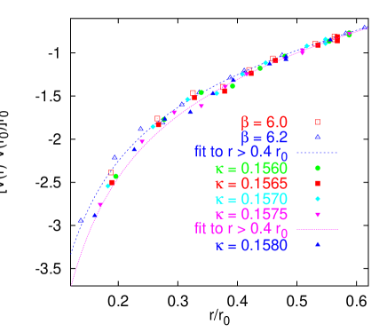
FIG. 14.: The short distance potential: quenched (open symbols) vs. un-quenched (full symbols).

B Torelons

In view of the difficulties in detecting string breaking directly in the static potential, it might be illuminating to investigate the effect of including sea quarks on torelon masses [36]. Such numerical simulations have been pioneered by Kripfganz and Michael [50] on small lattice volumes some ten years ago. In pure gauge theories a torelon that winds around a dimension of extent $L_{\sigma}a$ will have a mass,

$$m_{T}=aL_{\sigma}\left[\sigma+\Delta\sigma(aL_{\sigma})\right],$$ (17)

in the limit of large volumes, $aL_{\sigma}\rightarrow\infty$. $\sigma$ should be the very same string tension that governs the static potential at large distances. The sub-leading finite size correction [51],

$$\Delta\sigma=-\frac{\pi}{3(aL_{\sigma})^{2}},$$ (18)

is expected from the bosonic string picture. The effect of this contribution, which has been accurately verified in $SU(2)$ gauge theory [52], ranges from a decrease by 11 % on our smallest physical volume ($16^{3}$ at $\kappa=0.1575$) to 4.9 % on our biggest volume ($24^{3}$ at $\kappa=0.1575$).

In a pure gauge theory the centre symmetry of the action implies that all torelons that wind once around a lattice boundary are mass degenerate (see e.g. Appendix D.2 of Ref. [5] for details). When explicitly violating the centre symmetry by including sea quarks the degeneracy will be broken, with torelons to be classified in accord to representations of the cubic group, $O_{h}$ times charge conjugation. While in pure gauge theories glueballs can only split up into pairs of torelons, with sea quarks a single torelon can mix with or decay into a glueball that is in the same representation. For this to happen the torelon has to break up, unwind and rearrange itself into a flux loop with trivial winding number. In reality, one will meet different states (and creation operators) with equal quantum numbers. The operator that corresponds to the torelon in the quenched case will have maximal overlap with the state that is most torelon like but will in general, in the limit of large Euclidean times, decay into the lightest possible state. In the case that another state turns out to be lighter than the expected torelon mass we would call this effect “string breaking” of the torelon.

Heuristically one would expect a torelon-type operator to project better onto a state with a large mesonic component than a state with a large glueball component since the former appears as an intermediate state in the deformation of a torelon into a glueball anyway. On the other hand progress is being made in the excitation of flavour singlet states by use of mesonic operators (quark loops) [53, 10, 54] and there are indications [10] that purely gluonic operators of the type we use as well as mesonic operators might both have acceptable overlaps with the physical ground state.

TABLE VIII.: Torelon masses.

$\kappa$	$L_{\sigma}$	$m_{A_{1}^{++}}r_{0}$	$m_{E^{++}}r_{0}$	$m_{T_{1}^{+-}}r_{0}$	expected	$2m_{\pi}r_{0}$
0.1560	16	3.98(30)	4.03(20)	3.84(32)	3.78(07)	4.56(4)
0.1565	16	3.34(36)	3.43(25)	3.59(42)	3.59(11)	4.22(6)
0.1570	16	3.53(25)	3.54(19)	3.06(33)	3.51(14)	3.77(6)
0.1575	16	2.85(17)	2.82(15)	2.82(18)	3.11(12)	3.32(5)
0.1575	24	4.41(68)	6.16(66)	4.06(63)	5.03(08)	3.26(3)
0.1580	24	6.11(93)	5.36(44)	2.24(98)	4.71(13)	2.47(5)

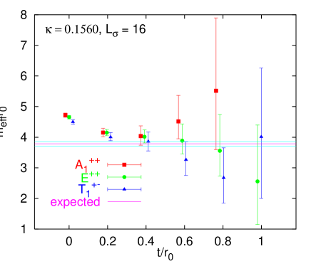
FIG. 15.: Effective torelon masses at $\kappa=0.156$, in comparison with the expectation, Eqs. (17) – (18), with the effective string tension $\sigma$ obtained from a fit to the static potential.

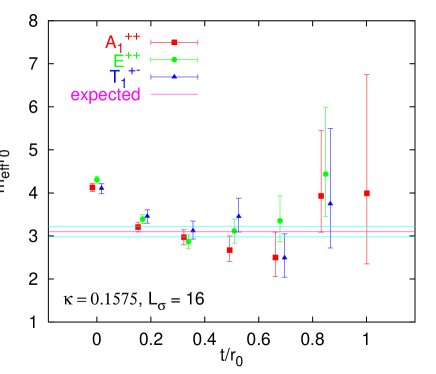
FIG. 16.: Same as Fig. 15 at $\kappa=0.1575$.

In addition to the fitted torelon masses, we display the non-string breaking expectations of Eqs. (17) – (18) in Tab. VIII, based on the string tensions from our four-parameter fits to the static potential of Tab. V. Unfortunately, the signals on the large lattices become very noisy, due to the larger torelon mass. Apart from isoscalar meson/glueball states, the $A_{1}^{++}$ torelon can in principle decay into a pair of $\pi$’s. We therefore include for guidance twice the $\pi$ mass in the last column of the Table. As we shall see below (Tab. IX), on all $16^{3}$ lattices, the scalar glueball comes out to have a mass very close to the torelon mass expectation of Eqs. (17) and (18). On our $24^{3}$ lattices, however, the expectation supercedes the $0^{++}$ and, eventually, the $1^{+-}$ glueball masses: breaking of the $A_{1}^{++}$ and, eventually, $T_{1}^{+-}$ torelons into a flavour singlet meson/glueball state becomes energetically possible. At the same time two $\pi$’s drop below the torelon expectation (and become lighter than the flavour singlet meson/glueball state).

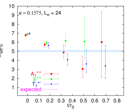
FIG. 17.: Same as Fig. 16 on the larger volume.

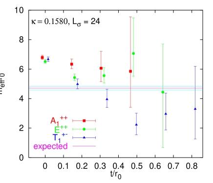
FIG. 18.: Same as Fig. 17 at $\kappa=0.158$.

On all the $16^{3}$ lattices, within statistical errors, the three torelons are mass degenerate and in agreement with the non-string breaking expectation. Two effective mass plots are displayed as examples in Figs. 15 and 16. The same holds true, within larger errors, in the case of the $24^{3}$ simulation at $\kappa=0.1575$ (Fig. 17). However, at $\kappa=0.158$ with a mass of $(2.24\pm 0.98)\,r_{0}$ at least the $T_{1}^{+-}$ torelon appears to fall short of the expectation by two and a half standard deviations (Fig. 18)! It would be important to increase statistics in order to corroborate this result as a signal for string breaking.

C Glueballs

We display the extracted masses of the three glueballs that we investigated in Tab. IX. The quenched results at a similar lattice spacing ($\beta=6.0$) have been calculated by Michael and Teper [42]. The quenched continuum $0^{++}$ result [5] (last row of the Table) stems from a quadratic extrapolation in the lattice spacing of data obtained in Refs. [55, 56, 42, 2, 57] while the tensor and axialvector results are from Morningstar and Peardon [4].

FIG. 19.: Effective $1^{+-}$ glueball masses. The horizontal line corresponds to the quenched continuum result.

FIG. 20.: Results on scalar and tensor glueball masses. The horizontal lines with error bands indicate quenched continuum results while the leftmost data points correspond to quenched Wilson action results obtained at finite lattice spacing ($\beta=6.0$). The expected torelon masses on $16^{3}$ and $24^{3}$ lattices are shown too (open triangles).

Effective mass plots of the scalar and tensor channels are shown in Figs. 1 – 6. In the case of $J^{PC}=1^{+-}$ no plateau has been established and the values displayed in the Table only represent upper limits. The corresponding effective masses are displayed in Fig. 19, in comparison to the continuum limit extrapolated quenched result (horizontal line with error band). Quenched results obtained at similar lattice spacings [42] suggest the glueball to lie somewhere inbetween $6.5\,r_{0}^{-1}$ and $8.5\,r_{0}^{-1}$ and, within statistical errors, do not deviate from the continuum value. Keeping in mind that all un-quenched simulations are statistically independent of each other, there is a clear indication for a $1^{+-}$ state being lighter than $6\,r_{0}^{-1}$. It remains to be demonstrated in future simulations at different lattice couplings, $\beta$, whether this conclusion persists in the continuum limit.

In Fig. 20, our results on the scalar and tensor glueballs are summarised. The leftmost data points represent the $\beta=6.0$ quenched results while the horizontal error bands correspond to the respective quenched continuum limits. The quenched scalar glueball at the finite lattice spacing comes out to be lighter by 15–20 % than the continuum limit extrapolated value [2, 5] while the tensor glueball is in agreement with the continuum result. In addition to the glueball masses, the torelon mass expectations of Eqs. (17) – (18) are included into the Figure. For $\kappa\leq 0.157$, $2m_{\pi}$ is larger than the torelon mass. On the $16^{3}$ lattice at $\kappa=0.1575$ the two masses come out to be degenerate within errors and on both $24^{3}$ lattices two $\pi$’s become lighter than the torelon (and the scalar glueball).

TABLE IX.: Glueball masses. A star indicates that no effective mass plateau could be identified and, therefore, only an upper limit is stated.

$\kappa$	$L_{\sigma}$	$m_{0^{++}}r_{0}$	$m_{2^{++}}r_{0}$	$m_{1^{+-}}r_{0}$	$m_{2^{++}}/m_{0^{++}}$
0.1560	16	3.56(12)	5.77(19)	5.0(2.1)*	1.62(07)
0.1565	16	3.72(46)	4.97(106)	8.1(1.2)*	1.34(34)
0.1570	16	3.02(18)	5.70(19)	4.6(1.2)*	1.89(13)
0.1575	16	3.26(25)	6.06(23)	12.7(2.3)*	1.86(13)
0.1575	24	4.21(35)	5.90(82)	6.2(2.3)*	1.41(23)
0.1580	24	3.85(38)	6.65(36)	4.8(1.8)*	1.72(17)
$\beta=6.0$	16	3.57(21)	5.70(32)	7.5(1.1)	1.60(14)
$\beta=\infty$	—	4.36(7)	5.85(8)	7.18(8)	1.34(3)

We do not detect any statistically significant deviation between quenched and un-quenched results in the $2^{++}$ channel. Unfortunately, the statistical error on the $24^{3}$ lattice at $\kappa=0.1575$ is too large to resolve possible finite size effects. We find all $16^{3}$ $0^{++}$ glueball data to roughly agree with the quenched $\beta=6.0$ result. At the same time, within statistical errors, the scalar glueball masses are degenerate with the $A_{1}^{++}$ (expected and measured) torelon masses. This degeneracy has also been observed in Ref. [50], on small lattice volumes: in the quenched approximation, finite size effects are small as long as two torelons are heavier than the glueball, however, with sea quarks, there is no protection preventing the glueball to decay into a single torelon. This could explain why the $0^{++}$ glueball on the 2 fm lattice at $\kappa=0.1575$ comes out to be significantly heavier than the one on the 1.4 fm lattice. Note that the size of the corresponding wave function becomes reduced when increasing the lattice volume (Sect. III).

On both $24^{3}$ lattices the mass of the scalar glueball comes out to be bigger than $2m_{\pi}$. There is no physical reason why the creation operator employed should have zero overlap with either a pair of $\pi$’s or a hypothetical $\pi\pi$ bound state [58]. However, it seems that this overlap is small, similar to the situation of the static potential, in which the smeared Wilson loop only receives a tiny contribution from pairs of static-light states. In conclusion, the mass of the state onto which the scalar glueball operator dominantly projects is compatible with quenched glueball results obtained at $\beta\geq 6$. We find finite size effects that can be interpreted as mixing with torelon states.

V Summary and Discussion

We have determined various “pure gauge” quantities in a simulation of QCD. Including two sea quark flavours results in a shift of about 10 % in $\beta$ and in an increase of the effective Coulomb strength, governing the interquark potential at $r>0.2$ fm, by 16 – 33 %, in the limit of light quark masses. While we have not been able to establish string breaking either in the ground state or in the $\Pi_{u}$ hybrid potential, a comparison of the ground state overlaps with quenched reference data suggests an effect at large distances.

Around $r_{c}\approx 2.3\,r_{0}\approx 1.15$ fm string breaking will become energetically possible for both potentials, ground state and hybrid, at $\kappa=0.1575$. On the assumption that reducing the bare quark mass, $m=(\kappa^{-1}-\kappa_{c}^{-1})/(2a)$, by an amount, $\Delta m$, induces an equal change in the static-light meson mass, we would guesstimate the string breaking length scale to drop by $\Delta r\approx 2\Delta m/\sigma\approx 0.18\,r_{0}$ when extrapolating to the physical sea quark mass. This crude estimate tells us that with two light quark flavours the QCD potential should become flat around $r_{c}\approx 1.05$ fm, such that in “real” $2+1$ flavour QCD string breaking at distances of 1 fm or smaller is likely.

For $\kappa\leq 0.1575$ torelon masses are in agreement with the (non-string breaking) expectation in terms of the effective string tension, obtained from a fit to the static potential, while at $\kappa=0.158$ there are indications for the torelon in one particular representation to become lighter than one would naïvely have expected. The basic problem is that we are only faced with a small window of lattice volumes for observation of “string breaking”. On a large lattice torelons become so heavy that the correlation functions disappear into noise at small temporal separation while on a small lattice the expected mass does not yet sufficiently differ from the masses of decay candidates to resolve an effect. It would be helpful in this respect to have for instance $\kappa=0.1575$ data at $L_{\sigma}=20$. The tensor glueball comes out to be heavier than the respective torelon state, i.e. in this case the two creation operators have little overlap with each other.

On our largest lattice ($\kappa=0.1575$) that corresponds to $m_{\pi}/m_{\rho}=0.704(5)$ with extent, $L_{\sigma}a\approx 4.07\,r_{0}$, we find, $m_{0^{++}}=4.21(35)\,r_{0}^{-1}$, which is in agreement with the quenched continuum limit result, $m_{0^{++}}=4.36(7)\,r_{0}^{-1}$. The $2^{++}$ glueball masses also seem to agree with the quenched results while there are indications for a light $T_{1}^{+-}$ glueball. On small lattices we find the scalar glueball and torelon to be degenerate and the glueball mass is underestimated. To exclude such finite size effects, the spatial lattice extent should be taken to be bigger than about $3.5\,r_{0}\approx 1.75$ fm.

Previous results with two flavours of Kogut-Susskind fermions have been obtained by the HEMCGC Collaboration [9] at the somewhat more chiral values [59], $m_{\pi}/m_{\rho}=0.658(5)$ and $m_{\pi}/m_{\rho}=0.434(4)$ on lattices with similar resolution as in the present study, $r_{0}\approx 5a$. Their lattice extents are [18], $L_{\sigma}a=3.08(12)\,r_{0}$ and $L_{\sigma}=2.50(5)\,r_{0}$, respectively, and, despite the rather small volume in the latter case and the extremely light quarks in the former case, the results [9, 18], $m_{0^{++}}=4.47(43)\,r_{0}^{-1}$ and $m_{0^{++}}=4.17(30)\,r_{0}^{-1}$, are compatible with ours.

Recently, the UKQCD Collaboration has reported first results for the scalar glueball, obtained with the Sheikholeshlami-Wohlert action on lattices with the linear dimension, $L_{\sigma}a\approx 3.4\,r_{0}$, at chiralities within the range explored in our study, as indicated by the ratios [10], $m_{\pi}/m_{\rho}\approx 0.71$ and $m_{\pi}/m_{\rho}\approx 0.67$. However, their lattices are quite coarse: $r_{0}\approx 3.44\,a$ and $r_{0}\approx 3.65\,a$, respectively. The values they state are remarkably small, namely $m_{0^{++}}=1.6(2)\,r_{0}^{-1}$ and $m_{0^{++}}=1.8(4)\,r_{0}^{-1}$, i.e. they come out to be by a factor two smaller than our $16^{3}$ lattice results, indicating larger finite lattice spacing effects than seen in quenched simulations [5, 10]. This issue certainly deserves further study.

At sufficiently light sea quark masses we expect the scalar glueball to mix with either flavour singlet mesonic states and eventually $\pi\pi$ molecules or to decay into $\pi$ pairs. Such scenarios should be studied, in un-quenched as well as quenched simulations [8, 58]. In view of the mixing and decay channels that open up once sea quarks are switched on, it is certainly also worthwhile to investigate glueballs with other quantum numbers than those that we have studied so far. In particular the pseudoscalar should be an interesting candidate, given the large mass of the $\eta$ meson. In view of fragmentation models as well as achieving an understanding of the decay rates of $\Upsilon(4S)$ and $\Upsilon(5S)$ states into pairs of $B\bar{B}$ mesons, a determination of the string breaking distance and the associated mixing matrix elements is certainly equally exciting. Work along this line is in progress [16, 45].

- [1] H. Fritzsch, M. Gell-Mann and H. Leutwyler, Phys. Lett. B47 (1973) 365.
- [2] G. S. Bali, K. Schilling, A. Hulsebos, A. C. Irving, C. Michael and P. W. Stephenson [UKQCD Collaboration], Phys. Lett. B309, 378 (1993) [hep-lat/9304012].
- [3] J. Sexton, A. Vaccarino and D. Weingarten, Phys. Rev. Lett. 75, 4563 (1995) [hep-lat/9510022].
- [4] C. J. Morningstar and M. Peardon, Phys. Rev. D60, 034509 (1999) [hep-lat/9901004].
- [5] G. S. Bali, submitted to Phys. Rept. [hep-ph/0001312].
- [6] F. E. Close, Nucl. Phys. A623 (1997) 125C [hep-ph/9701290].
- [7] S. Aoki et al. [CP-PACS Collaboration], Phys. Rev. Lett. 84, 238 (2000) [hep-lat/9904012].
- [8] W. Lee and D. Weingarten, Phys. Rev. D61, 014015 (2000) [hep-lat/9910008].
- [9] K. M. Bitar et al. [HEMCGC Collaboration], Phys. Rev. D44, 2090 (1991).
- [10] C. Michael, M. S. Foster and C. McNeile [UKQCD collaboration], hep-lat/9909036.
- [11] S. Güsken, hep-lat/9906034.
- [12] S. Güsken et al. [SESAM Collaboration], Phys. Rev. D59, 114502 (1999).
- [13] G. S. Bali and K. Schilling, Phys. Rev. D46, 2636 (1992).
- [14] G. S. Bali and K. Schilling, Phys. Rev. D47, 661 (1993) [hep-lat/9208028].
- [15] S. P. Booth, D. S. Henty, A. Hulsebos, A. C. Irving, C. Michael and P. W. Stephenson [UKQCD Collaboration], Phys. Lett. B294, 385 (1992) [hep-lat/9209008].
- [16] K. Schilling, hep-lat/9909152.
- [17] K. D. Born, E. Laermann, R. Sommer, P. M. Zerwas and T. F. Walsh, Phys. Lett. B329, 325 (1994).
- [18] U. M. Heller, K. M. Bitar, R. G. Edwards and A. D. Kennedy [HEMCGC Collaboration], Phys. Lett. B335, 71 (1994) [hep-lat/9401025].
- [19] U. Glässner et al. [SESAM Collaboration], Phys. Lett. B383, 98 (1996) [hep-lat/9604014].
- [20] G. S. Bali et al. [SESAM Collaboration], Nucl. Phys. Proc. Suppl. 63, 209 (1998) [hep-lat/9710012].
- [21] S. Güsken, Nucl. Phys. Proc. Suppl. 63, 16 (1998) [hep-lat/9710075].
- [22] J. Garden [UKQCD Collaboration], hep-lat/9909066.
- [23] S. Aoki et al. [CP-PACS Collaboration], Nucl. Phys. Proc. Suppl. 73, 216 (1999) [hep-lat/9809185].
- [24] C. Bernard et al. [MILC Collaboration], hep-lat/0002028.
- [25] T. Lippert et al., Nucl. Phys. Proc. Suppl. 60A, 311 (1998) [hep-lat/9707004].
- [26] L. A. Griffiths, C. Michael and P. E. Rakow, Phys. Lett. B129, 351 (1983).
- [27] G. S. Bali et al. [SESAM Collaboration], Nucl. Phys. Proc. Suppl. 53, 239 (1997) [hep-lat/9608096].
- [28] G. S. Bali, hep-ph/9809351.
- [29] G. S. Bali, Fizika B8, 229 (1999) [hep-lat/9901023].
- [30] SESAM and TL Collaborations, in preparation.
- [31] R. Sommer, Nucl. Phys. B411, 839 (1994) [hep-lat/9310022].
- [32] B. Allés et al. [TL Collaboration], Phys. Rev. D58, 071503 (1998) [hep-lat/9803008].
- [33] T. Lippert et al. [TL Collaboration], Nucl. Phys. Proc. Suppl. 73, 521 (1999) [hep-lat/9809034].
- [34] G. S. Bali, K. Schilling and A. Wachter, Phys. Rev. D56, 2566 (1997) [hep-lat/9703019].
- [35] S. Collins, C. Davies and G. Bali [UKQCD Collaboration], Nucl. Phys. Proc. Suppl. 63, 335 (1998) [hep-lat/9710058].
- [36] C. Michael, Phys. Lett. B232, 247 (1989).
- [37] B. Berg and A. Billoire, Nucl. Phys. B221, 109 (1983).
- [38] M. Albanese et al. [APE Collaboration], Phys. Lett. B192, 163 (1987).
- [39] M. Teper, Phys. Lett. B183, 345 (1987).
- [40] N. A. Campbell, L. A. Griffiths, C. Michael and P. E. Rakow, Phys. Lett. B142, 291 (1984).
- [41] P. de Forcrand and K. Liu, Phys. Rev. Lett. 69, 245 (1992).
- [42] C. Michael and M. Teper, Nucl. Phys. B314, 347 (1989).
- [43] R. Gupta, A. Patel, C. F. Baillie, G. W. Kilcup and S. R. Sharpe, Phys. Rev. D43, 2301 (1991).
- [44] S. Aoki et al. [CP-PACS Collaboration], Phys. Rev. D60, 114508 (1999) [hep-lat/9902018].
- [45] SESAM and TL Collaborations, in preparation.
- [46] P. Pennanen and C. Michael [UKQCD Collaboration], hep-lat/0001015.
- [47] C. DeTar, U. Heller and P. Lacock, hep-lat/9909078.
- [48] N. Eicker et al. [SESAM collaboration], Phys. Rev. D59, 014509 (1999) [hep-lat/9806027].
- [49] G. S. Bali and P. Boyle, Phys. Rev. D59, 114504 (1999) [hep-lat/9809180].
- [50] J. Kripfganz and C. Michael, Nucl. Phys. B314, 25 (1989).
- [51] J. Ambjørn, P. Olesen and C. Peterson, Nucl. Phys. B244, 262 (1984).
- [52] C. Michael and P. W. Stephenson [UKQCD Collaboration], Phys. Rev. D50, 4634 (1994) [hep-lat/9403004].
- [53] A. Ali Khan et al. [CP-PACS Collaboration], hep-lat/9909045.
- [54] SESAM Collaboration, in preparation.
- [55] P. de Forcrand, G. Schierholz, H. Schneider and M. Teper, Phys. Lett. B152, 107 (1985).
- [56] C. Michael and M. Teper, Phys. Lett. B206, 299 (1988).
- [57] A. Vaccarino and D. Weingarten, Phys. Rev. D60, 114501 (1999) [hep-lat/9910007].
- [58] M. Alford and R. L. Jaffe, hep-lat/0001023.
- [59] K. M. Bitar et al. [HEMCGC Collaboration], Phys. Rev. D49, 6026 (1994) [hep-lat/9311027].