Free energy of an SU(2) monopole-antimonopole pair.

Abstract

We present a high-statistic numerical study of the free energy of a monopole-antimonopole pair in pure SU(2) theory. We find that the monopole-antimonopole interaction potential exhibits a screened behavior, as one would expect in presence of a monopole condensate. Screening occurs both in the low-temperature, confining phase of the theory, and in the high-temperature deconfined phase, with no evidence of a discontinuity of the screening mass across the transition. The mass of the object responsible for the screening at low temperature is approximately twice the established value for the lightest glueball, indicating a prevalent coupling to glueball excitations. At high temperature, the screening mass increases. We contrast the behavior of the quantum system with that of the corresponding classical system, where the monopole-antimonopole potential is of the Coulomb type.

1 Introduction.

It is well known that some Higgs theories with non-Abelian gauge group admit stable monopole solutions [1, 2]. In certain cases, most notably in grand unified theories, the residual unbroken gauge group is non-Abelian. It is then particularly interesting to study the interaction between two monopoles, or between monopole and antimonopole, induced by the quantum fluctuations of the unbroken gauge group. Beyond the relevance that these interactions may have for the original theory, they can help clarify the low energy properties of the residual theory itself: from the point of view of the low energy theory, monopoles are point-like external sources of non-Abelian gauge field, so they act as non-trivial probes of the strong coupling dynamics. Indeed, already some time ago t’Hooft [3] and Mandelstam [4] proposed that condensation of magnetic monopoles could be responsible for the confinement mechanism [5]. If the vacuum state of a non-Abelian gauge theory is characterized by the presence of a monopole condensate, this will screen the monopole-antimonopole interaction, which should therefore exhibit a Yukawa-like behavior. If there is no condensate whatever, one should expect instead a Coulombic interaction between the monopoles, as is the case in classical SU(2) theory. Finally, in a theory characterized by a condensation of electric charges, the monopole-antimonopole interaction energy should increase linearly with separation. While a substantial of work has already been done to understand the role of monopole condensation for the confinement mechanism [6, 7, 8, 9, 10, 11, 12], to the best of our knowledge a precise determination of the monopole-antimonopole interaction potential in a quantum non-Abelian theory is still lacking. In this paper we plan to fill this void, presenting a numerical calculation of the monopole-antimonopole potential in the $SU(2)$ theory. Our results show that the monopole-antimonopole interaction potential is screened, buttressing the conjecture of a monopole condensate. We also study the monopole-antimonopole system in the high-temperature, deconfined phase of SU(2). The interaction still exhibits screening, which can be ascribed to a magnetic mass. We will investigate the temperature dependence of this mass.

2 Monopole-antimonopole configuration and calculation of the free energy.

The procedure for introducing $SU(N)$ monopole sources on the lattice was devised by Ukawa, Windey and Guth [13] and Srednicki and Susskind [14], who built on earlier seminal results by t’Hooft [15], Mack and Petkova [16, 17] and Yaffe [18]. In this paper we will follow the method of Ref. [14]. In three dimensions, an external monopole-antimonopole pair can be introduced by “twisting” the plaquettes transversed by a string joining the monopole and the antimonopole (see Fig. 1), i.e. by changing the coupling constant of these plaquettes according to $\beta$ to $z_{n}\beta$, where $z_{n}=\exp(2\pi\imath n/N)$ is an element of the center of the group . The location of the string is unphysical. It can be changed by redefining link variables on the plaquettes transversed by the string by $U\to z_{n}^{-1}U$, as illustrated in Fig. 2. The fact that $z_{n}$ is an element of the center $SU(N)$ guarantees that the above redefinition is a legitimate change of variables. On the other hand, the position of the cubes that terminate the string cannot be changed. Those cubes contain two external monopoles of charge $z_{n}$ and $z_{n}^{-1}$ respectively (or, equivalently, a monopole of charge $z_{n}$ and its antimonopole). In the $SU(2)$ theory we consider in this paper, the only non-trivial element of the center of the group is $z=-1$ and thus monopole and antimonopole coincide.

Figure 1: Monopole antimonopole pair induced by twisting the plaquettes transversed by the string.

Figure 2: Change of the string location brought about by the redefinition of the gauge variable on the link denoted by a bolder line.

In four dimensions, a static monopole-antimonopole pair is induced by replicating the string on all time slices. The insertion of a monopole-antimono-pole pair can be reinterpreted in terms of the electric flux operator and several investigations have been devoted to the study of such operator (see for instance Refs. [20, 21]). However, as we already stated, accurate numerical information on the free energy of a monopole-antimonopole has never been obtained.

The numerical calculation of a free energy by stochastic simulation can be a quite challenging problem, since the free energy is related to the partition function and the partition function, which is the normalizing factor for the simulation, cannot be directly measured. In our case, we need the ratio of the partition functions of a system containing the monopole-antimonopole pair to the partition function of the free system. In order to calculate this quantity we define a generalized system where the coupling constant $\beta$ has been replaced by ${\beta^{\prime}}$ on all the plaquettes transversed by the string. For sake of precision, if we place the monopole at the spatial location of integer value coordinates $x_{0}+\frac{1}{2},y_{0}+\frac{1}{2},z_{0}+\frac{1}{2}$ and the antimonopole at $x_{0}+\frac{1}{2},y_{0}+\frac{1}{2},z_{0}+d+\frac{1}{2}$, the plaquettes with coupling ${\beta^{\prime}}$ will be all the $x$-$y$ plaquettes with lower corner in $x_{0},y_{0},z,t$, where $z_{0}+1\leq z\leq z_{0}+d$ and $0\leq t\leq N_{t}-1$. $N_{x},N_{y},N_{z},N_{t}$ denote the extents of the lattice in the four dimensions. The $\frac{1}{2}$ offsets in the coordinates of the monopole and antimonopole are due to the fact that we consider them located at the center of two spatial cubes, namely those with lowest corners in $x_{0},y_{0},z_{0}$ and $x_{0},y_{0},z_{0}+d$, respectively. For the monopole-antimonopole configuration we use periodic boundary conditions. We will also consider single monopole configurations. For these we use periodic boundary conditions only in time and the two spatial directions orthogonal to the string, while we choose free boundary conditions in the spatial direction parallel to the direction of the string. We let the string run from the mid-point of the lattice to the free boundary. This places a single monopole in the middle of the lattice and emulates as well as possible a configuration where the antimonopole has been removed to infinity.

Let us denote by $M$ the set of all the plaquettes with modified coupling constant. The action of the modified system is then

$$S(\beta,{\beta^{\prime}})=\frac{1}{2}\left(\beta\sum_{P\not\in M}\mbox{Tr}(U_{P})+{\beta^{\prime}}\sum_{P\in M}\mbox{Tr}(U_{P})\right)$$ (1)

and the corresponding partition function is

$$Z(\beta,{\beta^{\prime}})=\sum_{\mathcal{C}}e^{-S(\beta,{\beta^{\prime}})}$$ (2)

where ${\mathcal{C}}$ denotes the set of all configurations. For ${\beta^{\prime}}=\beta$ our generalized system obviously reduces to a homogeneous $SU(2)$ lattice gauge system with coupling constant $\beta$, whereas for ${\beta^{\prime}}=-\beta$ it becomes an $SU(2)$ model with a static monopole-antimonopole pair. In this latter case, as discussed above, the partition function becomes independent on the actual location of the string, and depends only on the distance $d$ between monopole and antimonopole (beyond depending, of course, on $\beta$ and the extent of the lattice). The change of free-energy induced by the presence of the pair is thus

$$F=-T\log\frac{Z(\beta,-\beta)}{Z(\beta,\beta)}$$ (3)

where $T=N_{t}a$ is the temperature of the system ($a$ denotes, as usual, the lattice spacing). This is the quantity we want to calculate. For ${\beta^{\prime}}$ not equal to $\beta\ \rm{or}\ -\beta$, $Z(\beta,{\beta^{\prime}})$ does depend on the location of the string. Nevertheless Eq. 2 continues to define the partition function of a statistical system, which we will use for our calculation of $F$. The basic idea is that we will perform Monte Carlo simulations of the modified system for a set of values of ${\beta^{\prime}}$ ranging from $\beta$ to $-\beta$ which is sufficiently dense that for all steps in ${\beta^{\prime}}$ we can reliably estimate the change induced in $\log Z$. Conceptually this corresponds to the observation that for an infinitesimal change in ${\beta^{\prime}}$ the change in free energy will be

$$\frac{\partial F_{\beta^{\prime}}}{\partial{\beta^{\prime}}}=\frac{1}{2}\langle\sum_{P\in M}\mbox{Tr}(U_{P})\rangle_{\beta^{\prime}}$$ (4)

and thus the free energy of the monopole pair can be computed as

$$F=\int_{-\beta}^{\beta}d{\beta^{\prime}}\,\frac{\partial F_{\beta^{\prime}}}{\partial{\beta^{\prime}}}=\frac{1}{2}\int_{-\beta}^{\beta}d{\beta^{\prime}}\,\langle\sum_{P\in M}\mbox{Tr}(U_{P})\rangle_{\beta^{\prime}}$$ (5)

where the integrand in the r.h.s. is an observable, namely the energy

$$E=\frac{1}{2}\langle\sum_{P\in M}\mbox{Tr}(U_{P})\rangle_{\beta^{\prime}}$$ (6)

of the strip of plaquettes transversed by the string. However, implementing Eq. 5 would be inefficient, due to the large number of subdivisions that the numerical integration would require for accuracy. Rather, we calculate $F$ by following the Ferrenberg-Swendsen multi-histogram method [22].

Following Ref. [22], we choose a set of $N+1$ values $\{{\beta^{\prime}}_{i}\}$ ranging from ${\beta^{\prime}}_{0}=\beta$ to ${\beta^{\prime}}_{N}=-\beta$. In the actual calculation, we chose them equally spaced, although this is not necessary. The number $N$ is determined by a criterion that will be explained below. For each value ${\beta^{\prime}}_{i}$ we perform a Monte Carlo simulation of the corresponding system and record the values of the energy $E$ of the plaquettes transversed by the string (see Eq. 6) in a histogram $h_{i}(E)$. More exactly, in our calculation rather than simply accumulating the entries in the histograms, we distributed the measured energy values over the four neighboring vertices according to the weights of a cubic interpolation formula. This substantially increases the accuracy when the values in the histograms are subsequently used to approximate integrals over the density of states: $\int\rho(E)f(E)dE\approx Z\sum_{E}(h(E)/n)f(E)$, $n$ being the total number of entries in the histogram. Indeed, by using this procedure, we were able to reduce the number of bins to $200$ without noticeable discretization effects.

From each separate histogram one can obtain an independent estimate of the density of states

$$\frac{\rho_{i}(E)}{Z_{i}}=\frac{h_{i}(E)}{n_{i}}e^{{\beta^{\prime}}_{i}E}$$ (7)

where $Z_{i}$ is the partition function for the specific value ${\beta^{\prime}}_{i}$ and $n_{i}$ is the total number of histogram entries. Of course, the normalizing factors $Z_{i}$ are still not known. Indeed, the entire goal of the computation is to calculate the relative magnitude of the partition functions $Z_{i}$. Starting from Eqs. 7 one can however obtain the partition functions $Z_{i}$ up to a common constant of proportionality by a self-consistent procedure. We start from the crude approximation that all $Z_{i}$ are equal. Since we are only interested in ratios of partition functions, we can set this common value to 1. We combine then the estimates of the density of states given by Eqs. 7 into a first approximation

$$\rho(E)=\frac{1}{N}\sum_{i}\rho_{i}(E)$$ (8)

From this value of the density of states we can now obtain a better approximation of the partition functions

$$Z_{i}=\sum_{E}\rho(E)e^{-{\beta^{\prime}}_{i}E}$$ (9)

Equations (7-9) can now be iterated to get $Z_{i}$ up to a multiplicative factor. If the iterations converge, the final results will provide a self-consistent set of values for the partition functions $Z_{i}$, up to a common constant. In particular, we will be able to obtain $\frac{Z(\beta,-\beta)}{Z(\beta,\beta)}=\frac{Z_{N}}{Z_{0}}$ and the free energy of the monopole-antimonopole pair.

A necessary condition for the above procedure to work well is that the histograms corresponding to adjacent ${\beta^{\prime}}$ have a sufficient overlap. In fig. 3 we plot the histograms obtained in a typical run and one can see that they exhibit indeed a substantial overlap.

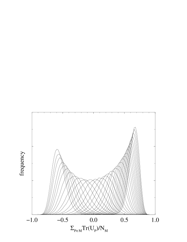
Figure 3: The overlap of histograms at $\beta=2.6$ and different $\beta^{\prime}$. The monopole separation is $2a$ and $N_{t}=6$.

In our calculation we found that the self-consistent procedure outlined above converged rapidly for all the values of lattice size, coupling constant and monopole-antimonopole separation we considered. We checked that the results for the free energy we obtained with the multihistogram method are consistent with the values one can obtain from the numerical integration of $\partial F_{\beta^{\prime}}/\partial\beta^{\prime}$ (cfr. Eq. 5), within the error of the latter procedure.

3 Computational details and numerical results.

We simulated a pure $SU(2)$ system with a combined overrelaxation and multihit-Metropolis algorithm for minimal autocorrelation time. We studied systems with coupling constants varying between $\beta=2.476$ and $\beta=2.82$, spatial sizes ranging from $16^{2}\times 32$ to $32^{2}\times 64$ and Euclidean temporal extents ranging from $16$ down to $2$. The corresponding temperatures span the deconfinement phase transition, which occurs at $N_{t}\approx 10$ for $\beta=2.6$ and between $N_{t}=7$ and $N_{t}=8$ for $\beta=2.476$ and $\beta=2.5$ [23]. Full details of lattice sizes and couplings used in our simulations are given in table 1. For each lattice size, value of $\beta$ and monopole separation, we performed a sequence of simulations, starting with ${\beta^{\prime}}=\beta$ and decreasing ${\beta^{\prime}}$ in steps (cfr. Sect. 2) to its final value ${\beta^{\prime}}=-\beta$. Precisely, we performed $5000$ thermalization steps at ${\beta^{\prime}}=\beta$ followed by measurements separated by $50$ updates. We decreased ${\beta^{\prime}}$, performed another $500$ thermalization followed by the same number of measurements, again separated by $50$ updates, and so on, until completion of the measurements with ${\beta^{\prime}}=-\beta$. For each measurement, as a variance reduction technique, we performed $384$ upgrades of the links in the plaquettes belonging to the flux tube $M$, while keeping all other link variables fixed. In this way, we obtained $384$ histogram entries per configuration.

$\beta$	$N_{x}\times N_{y}\times N_{z}$	$N_{t}$
2.82	$32\times 32\times 64$	4
2.6	$20\times 20\times 40$	2,4,6,16
2.5	$16\times 16\times 32$	4,12
2.476	$16\times 16\times 32$	4,12

Table 1: Lattice sizes and couplings at which the simulation was performed.

The number of measurements in each individual simulation, as well as the number of steps in ${\beta^{\prime}}$, depended on monopole separation and lattice size and are given in tables 2 and 3. In order to estimate the error we proceeded as follows. For all data we performed a standard jackknife evaluation of the error based on 10 subsamples. The data are however highly correlated and this leads to an underestimate of the error. An error analysis based on the full correlation matrix would have been computationally too costly. Instead, we performed seven totally independent calculations of the free energy for a few data points and calculated the error from the variance of the results. This came out approximately four times larger than the corresponding estimate of the error from the jackknife method. Thus we multiplied all of the jackknife errors by a factor of four. While this universal rescaling can only produce an approximation to the true errors, because the correlation in the data will generally vary from data point to data point, we feel that it gives the most realistic estimate of the actual errors that can be obtained without embarking in an error analysis of prohibitive cost. Our code was written in Fortran 90 and was run on the SGI-Origin 2000 at the Boston University Center for Computational Science. It performs at $\approx 140$ MFlops on a single 190MHz R10000 CPU and scales well up to 64 CPU’s. The total CPU-time needed for the simulations was $\approx 3\times 10^{4}$ CPU hours.

$d$	# ${\beta^{\prime}}$	# m	#${\beta^{\prime}}$	# m	#${\beta^{\prime}}$	# m	#${\beta^{\prime}}$	# m
1	11	200	11	600	11	600	11	800
2	21	200	21	600	21	600	21	800
3	31	200	31	600	31	600	31	800
4	41	200	41	600	41	600	41	800
5	51	200	51	600			51	600
6	51	200	61	600	61	600	61	800
$\infty$	101	200	101	600

Table 2: Computational details of the simulations at $\beta=2.6$, and $N_{t}=16,\;6,\;4,\;2$ (from left to right). $d$ is the monopole separation in lattice units, # ${\beta^{\prime}}$ is the number of ${\beta^{\prime}}$ steps and # m is the number of independent configurations per ${\beta^{\prime}}$, which measurements were taken over.

$d$	# ${\beta^{\prime}}$	# m	#${\beta^{\prime}}$	# m	#${\beta^{\prime}}$	# m	#${\beta^{\prime}}$	# m	#${\beta^{\prime}}$	# m
1	11	100	11	600	11	600	11	200	11	800
2	21	100	21	600	21	600	21	200	21	800
3	31	100	31	600	31	600	31	200	31	800
4	41	100	41	600	41	600	41	200	41	800
6	61	100	61	600	61	600	61	200	61	800

Table 3: Computational details of the simulations at $\beta=2.82,\;N_{t}=4$; $\beta=2.5,\;N_{t}=12$; $\beta=2.5,\;N_{t}=4$; $\beta=2.476,\;N_{t}=12$ and $\beta=2.476,\;N_{t}=4$ (from left to right).

We measured the free energy of the monopole-antimonopole pair for several values of lattice size, coupling constant $\beta$ and monopole-antimonopole separation $d$. Tables 4 and 5 list all our results.

$d$	$F[N_{t}=16]$	$F[N_{t}=6]$	$F[N_{t}=4]$	$F[N_{t}=2]$
1	1.3464(50)	1.3472(38)	1.3193(92)	1.0236(114)
2	1.6961(28)	1.6741(48)	1.5811(51)	1.1492(98)
3	1.7708(18)	1.7357(20)	1.6056(35)	1.1586(69)
4	1.7909(18)	1.7334(25)	1.6253(34)	1.1531(62)
5	1.7927(10)	1.7350(19)
6	1.7950(10)	1.7375(33)	1.6411(26)	1.1420(44)
$\infty$	1.7927(22)

Table 4: Free energy in units of $a^{-1}$ of the monopole-antimonopole pair at various separations $d$ for the confined ($N_{t}=16$) and deconfined ($N_{t}=6,4,2$) phases. Results are for spatial lattice size $N_{x}\times N_{y}\times N_{z}=20\times 20\times 40$ at $\beta=2.6$. The entry with separation $\infty$ is twice the energy of a single monopole as measured on a $N_{x}\times N_{y}\times N_{z}=20\times 20\times 20$ lattice and free boundary conditions in the $z$ direction.

$d$	$F[N_{t}=4]$	$F[N_{t}=12]$	$F[N_{t}=4]$	$F[N_{t}=12]$	$F[N_{t}=4]$
1	1.648(40)	1.1451(58)	1.1332(92)	1.0988(35)	1.0927(42)
2	2.037(28)	1.4020(33)	1.3549(41)	1.3241(24)	1.2885(53)
3	2.129(20)	1.4437(28)	1.3741(36)	1.3574(16)	1.3133(40)
4	2.222(16)	1.4601(24)	1.3806(37)	1.3736(14)	1.3188(26)
6	2.191(17)	1.4726(23)	1.3779(26)	1.3683(26)	1.3169(18)

Table 5: Free energy in units of $a^{-1}$ of the monopole-antimonopole pair at various separations $d$ at high temperature ($N_{t}=4$) on a $N_{x}\times N_{y}\times N_{z}=32\times 32\times 64$ lattice at $\beta=2.82$ (left), and for the confined ($N_{t}=12$) and deconfined ($N_{t}=4$) phases on a $N_{x}\times N_{y}\times N_{z}=16\times 16\times 32$ lattice at $\beta=2.5$ (middle) and $\beta=2.476$ (right).

Figure 4: Free energy of the monopole-antimonopole pair versus separation at $\beta=2.6$ for different values of $N_{t}$. The lines represent fits of the first 4 points to a Yukawa potential. The results of the fit for the screening mass $m$ are listed in table 6.

Typical results are illustrated in Figure 4, where we plot the data for the monopole-antimonopole free energy obtained at $\beta=2.6$. The flattening of the potential at large separation gives evidence for the screening of the interaction. The lines in the figure reproduce fits to a Yukawa potential

$$F(r)=F_{0}-c\frac{e^{-mr}}{r}$$ (10)

The fits give clear indications for a non-vanishing screening mass (see the tables for details) and rule out a Coulombic behavior of the potential.

We fit all of our data to a Yukawa potential, as in Eq. 10. We used the points at separation $d=1$ to $4$ for the fits. In the confined phase, it is also possible to perform meaningful fits through the points at separation $2$ to $6$, leaving out the point at $d=1$, where one expects the value of the potential to be most affected by lattice distortions. For higher temperatures the rapid flattening of the potential makes the fits more sensitive to the removal of the first point. An alternative procedure consists in fitting the data to a lattice Yukawa potential, as suggested in this context in Ref. [24]. The results of the fits for the screening masses are reproduced in Table 6. Unprimed (primed) quantities refer to the values obtained from fits to a continuum (lattice) potential of the data with $d$ ranging from $1$ to $4$. For the conversion in units of the string tension $\sqrt{\sigma}$ we used $a\sqrt{\sigma}=0.1989,0.1834,0.1326,0.0663$ for $\beta=2.476,2.5,2.6,2.82$, respectively. We took the values for $\beta=2.5,2.6$ from Ref. [25] and calculated the other values from the known scaling behavior of the theory. The fact that all fits produce a non-vanishing value for the screening mass is a clear indication that the data are not consistent with a Coulombic monopole-antimonopole interaction. To reinforce this point, we attempted a direct Coulombic fit to the data for $\beta=2.6$, $N_{t}=16,\;6$ and found the fit quality to be $Q\approx 10^{-62}$ for $N_{t}=16$ and $Q\approx 10^{-68}$ for $N_{t}=6$, definitely ruling out a Coulombic behavior of the potential in both phases.

$\beta$	$T/\sqrt{\sigma}$	$m/\sqrt{\sigma}$	$ma$	Q	$m^{\prime}/\sqrt{\sigma}$	$m^{\prime}a$	Q’
2.476	0.419	4.62(32)	0.918(64)	$0.003$	5.87(45)	1.168(89)	$0.0001$
2.5	0.454	5.04(43)	0.924(78)	0.16	6.43(60)	1.180(110)	0.06
2.6	0.472	5.79(31)	0.768(41)	0.54	7.21(40)	0.956(53)	0.67

$\beta$	$T/\sqrt{\sigma}$	$m/\sqrt{\sigma}$	$ma$	Q	$m^{\prime}/\sqrt{\sigma}$	$m^{\prime}a$	Q’
2.476	1.257	6.4(1.0)	1.28(20)	0.85	8.6(1.7)	1.71(34)	0.72
2.5	1.363	8.65(1.29)	1.59(24)	0.47	12.49(2.34)	2.29(43)	0.40
2.6	1.257	9.16(69)	1.22(9)	$0.0001$	11.86(1.11)	1.57(15)	$0.0004$

$\beta$	$N_{t}$	$T/\sqrt{\sigma}$	$m/\sqrt{\sigma}$	$ma$	$Q$	$m^{\prime}/\sqrt{\sigma}$	$m^{\prime}a$	Q’
2.6	4	1.885	8.9(1.2)	1.18(16)	$0.006$	12.0(2.0)	1.59(26)	$0.003$
2.6	2	3.771	18.5(8)	2.45(11)	0.53	31.3(17.3)	4.15(2.30)	0.53
2.82	4	3.771	7.9(2.6)	0.52(17)	0.08	8.4(3.0)	0.55(20)	0.12

Table 6: Screening masses from a Yukawa fit of the free energy in units of the zero-temperature string tension $\sqrt{\sigma}$ and in lattice units. For comparison, the temperature of the system in units of the zero-temperature string tension is also given. The first table is for confined systems at at comparable temperatures. The second table is for deconfined systems, again at comparable temperatures. The third table gives the screening masses for various high temperature simulations. $m$ and $m^{\prime}$ refer to the fits done with continuum and lattice potential, respectively. $Q$ and $Q^{\prime}$ are the corresponding qualities of the fit.

In table 7 we compare our values for the screening mass at $\beta=2.5$ and $\beta=2.6$ with with the values for the lightest glueball mass in the SU(2) theory [25, 26]. We reproduce the results from fits with the continuum Yukawa potential to the data points at separation $1$ through $6$ ($m_{1}$), from fits, always with the continuum potential, where we disregarded the points at separation $1$ which have the largest discretization error ($m_{2}$), and from fits to the points at separation $1$ through $6$ with the lattice Yukawa potential ($m^{\prime}$). The values $m_{2}$ and $m^{\prime}$ are consistent and are approximately twice as large as the mass of the lightest glueball. This indicates that the predominant coupling of the monopoles is to glueball excitations. Our results do not rule out that the lightest glueball may dominate screening at long distances, but this not visible within the range of lattice separations ($a-5a$) for which we can obtain sufficiently accurate results.

$\beta$	$m_{g}a$	$m_{1}a$	$m_{2}a$	$m^{\prime}a$	$Q(m_{1})$	$Q(m_{2})$	$Q(m^{\prime})$
2.6	0.51(3)	0.849(26)	1.019(14)	0.998(36)	0.08	0.52	0.59

Table 7: Comparison of screening masses and the lowest glueball mass $m_{g}a$ (taken from [25, 26]). The masses $m_{1}$ and $m_{2}$ are obtained from fits with the continuum Yukawa potential to the data points at separation $1$ through $6$ and $2$ through $6$, respectively. The masses $m^{\prime}$ are from fits with the lattice Yukawa potential to the data points at separation $1$ through $6$.

Figure 5: Screening mass vs. temperature at $\beta=2.6$. Because of the large systematic errors introduced by the small temporal lattice extent $N_{t}=2$ for the last data point, we also included results from simulation at the same physical volume and half the lattice spacing ($\beta=2.82$). The dashed line indicates the critical temperature (taken from [23]).

In figure 5 we plot our results for the screening mass $m$ vs. temperature. At high temperature $m$ should be identified with the magnetic screening mass. Our results are consistent with data obtained by Stack [27] by another method. They appear to be somewhat larger than the values for $m$ obtained, by a yet different technique, by Heller, Karsch and Rank [28]. The authors of Ref. [28] quote results, however, for systems with larger $N_{t}$ and higher $\beta$ than we generally used in our investigation. The closest comparison can be made between our result for $\beta=2.82$, namely $m/T=2.09(0.69)$, and the results in Ref. [28]: $m/T=2.01(0.29),1.24(0.04)$ for $\beta=2.74,2.88$ respectively. These latter sets of results are reasonably consistent. It is interesting that, within the accuracy of our data, there is no indication for a discontinuous behavior of $m$ at the deconfinement transition. The apparently continuous behavior of $m$ should not come, though, as a surprise. We should remember that the quantity we study is based on insertion in the SU(2) theory of an operator (the sheet of plaquettes with modified coupling joining the world line of the monopoles) which is dual to the $x-y$ Wilson loops [3]. Space-space Wilson loops exhibit an area law behavior both below and above the deconfinement transition and, correspondingly, one would expect that the free energy of monopole-antimonopole pair, whose propagation spans a dual space-time surface, should exhibit screened behavior on both sides of the phase transition. The discontinuity at the phase transition occurs in the behavior of space-time Wilson loops or in the correlation of timelike Polyakov loops. Accordingly, we would expect a discontinuity in the partition function of the system with the monopole-antimonopole pair propagating in the space direction. In order to test this idea, we also measured the partition function of a system where we changed the sign of the $t-y$ plaquettes crossing a string joining monopole and antimonopole separated by $d$ lattice sites in the $z$ direction and propagating in the $x$ direction. We performed the calculation at $\beta=2.6$ with a lattice of size $N_{x}=N_{y}=20,N_{z}=40,N_{t}=6$. While the physical meaning of the “free energy” $F=-(1/N_{x})\log[Z(\beta,-\beta)/Z(\beta,\beta)]$ become less obvious (it would be the free energy for a low-temperature system confined in a periodic box of width $N_{x}$), our results, listed in table 8 and illustrated in Fig. 6, show that above the phase transition this quantity does exhibit a confined behavior. The dashed line in the figure reproduces a fit of a Coulomb plus linear form $a+b/x+cx$ with parameters $a=2.107(2),b=0.658(3),c=0.0167(3)$. It is interesting to observe that from the fit we get $\sqrt{c}=0.1291(11)$, while the string tension on a $20^{4}$ lattice at the same value of $\beta$ is $a\sqrt{\sigma}=0.1326(30)$.

$d$	$F$
1	1.3640(13)
2	1.7396(10)
3	1.8512(15)
4	1.9180(13)
6	1.9948(6)
8	2.0756(6)

Table 8: Value of the spatial ’t Hooft loop in units of $a^{-1}$ at various separations $d$ for a deconfined system ($N_{t}=6$) with spatial lattice size $N_{x}\times N_{y}\times N_{z}=20\times 20\times 40$ at $\beta=2.6$.

Figure 6: Comparison of the “free energy” for propagation in the space direction vs. propagation in the time direction of the monopole-antimonopole pair, for a system in the deconfined phase.

It is interesting to compare our results to the solutions of the classical theory. Since to the best knowledge of the authors there is no analytical solution to the classical two monopole problem, we have investigated its properties numerically. To do this, we found the minimal energy solutions on a lattice and checked their behavior. We put the classical system on a 3-dimensional lattice with free boundary conditions. (We used free boundary condition because the calculation itself shows that the potential has a long range behavior and with free boundary conditions we can reduce finite size effects.) We started both from a random non-Abelian configuration and and from a random Abelian configuration and performed iterative local minimization to relax the system to its lowest energy state. There were no surprises as we found that for both initial conditions the system relaxed to a minimal energy state of the same energy and that the non-Abelian solution, after going to a maximally Abelian gauge, turned out to be entirely Abelian in nature. Also, the potential of interaction was well fit by the Coulomb form $V=1/(4r)$. (One expects a coefficient 1/4 in the Coulomb potential because the total magnetic flux from the monopole is $\Phi=\pi$. This value has been numerically confirmed in our calculation.)

Figure 7: Comparison of monopole-antimonopole potentials in the confined phase of the quantum system and in the classical system. Data for the quantum system are at $\beta=2.6$ and $N_{t}=16$.

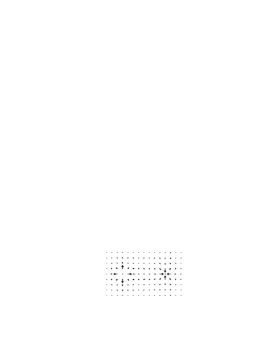
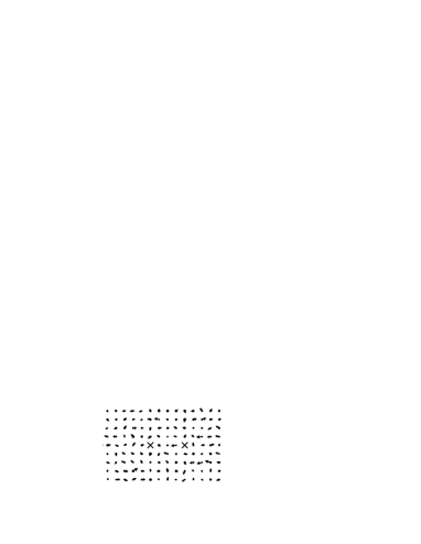
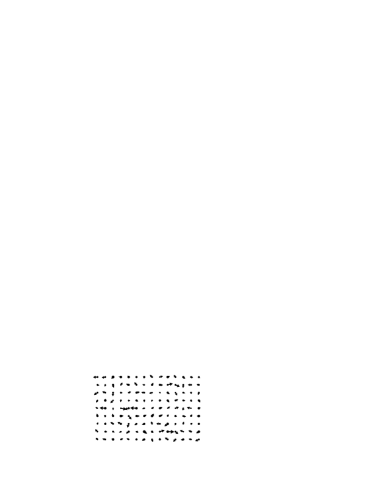
Figure 8: Comparison of the maximally Abelian projected configuration for the classical minimal energy solution (first picture) and an average over the time slices of a typical quantum configuration. The second picture is a detail of a region around the monopoles, the third one is from a region without monopoles.

In Figure 7 we compare the monopole-antimonopole potentials in the confined phase of the quantum system and in the classical system. The comparison shows a clear difference between the classical and quantum case and reinforces the conclusion that quantum fluctuations introduce a screening of magnetic monopoles. We further illustrate this point by displaying in Fig. 8 snapshots of a typical quantum configuration (from a simulation at $\beta=2.476$ and $N_{t}=12$) and of the classical solution. In the pictures, vectors show the magnetic field in a maximal Abelian projection and the size of the dots measure the non-Abelian character of the configuration at that point (it is proportional to the square of the components orthogonal to the Abelian projection). In the classical case the location of the monopole-antimonopole pair is evident. In the quantum case it is marked by the crosses in the middle of the second picture. Had we not marked the location of monopole and antimonopole in the quantum case, the reader would be hard pressed in finding where they are. The marked difference between the classical and quantum configurations gives a vivid illustration of how the quantum fluctuations of the gluon field provide a mechanism for the screening of external monopole sources, which is most likely also responsible for confinement in the low temperature phase and for the emergence of the magnetic mass in the high temperature phase.

4 Conclusions.

We have measured the free energy of a monopole-antimonopole pair in pure SU(2) gauge theory at finite temperature. We find that the interaction is screened in both the confined and deconfined phase. The mass of the object responsible for the screening at low temperature is approximately twice the established value for the lightest glueball, indicating a prevalent coupling to glueball excitations. There is no noticeable discontinuity in the screening mass at the deconfinement transition, but in the deconfined phase we clearly see an increase of the screening mass with temperature. Our results support the hypothesis of existence of monopole condensate in the vacuum of the SU(2) theory and provide evidence that some glueball excitation could serve as a “dual photon” in the dual superconductor hypothesis of quark confinement. Finally, we would like to observe that the method we have developed for the calculation of the monopole-antimonopole free energy is applicable to other models, beyond the SU(2) theory considered in this paper. While moderately demanding in computer resources, it appears capable of producing accurate numerical results for the monopole-antimonopole potential of interaction. Thus it could be used to shed light on the dynamics of other interesting systems that are expected to exhibit the formation of electric or magnetic condensates in their vacuum states.

Acknowledgments. We gratefully acknowledge conversations and exchanges of correspondence with Maxim Chernodub, Urs Heller, Chris Korthals Altes, Christian Lang, Peter Petreczky, Misha Polikarpov, John Stack, Matthew Strassler and Terry Tomboulis. We also grateful to Philippe de Forcrand for bringing to our attention a discrepancy between his own results for the monopole-antimonopole free energy and the values we presented in an earlier version of this paper, which helped us correct a programming error in the implementation of the multihistogram method, and for correspondence regarding the free energy of the space-like ’t Hooft loop. This research was supported in part under DOE grant DE-FG02-91ER40676 and by the U.S. Civilian Research and Development Foundation for Independent States of FSU (CRDF) award RP1-187.

References

- [1] G. ’t Hooft, Nucl. Phys. B79 (1974) 276.
- [2] A. M. Polyakov, JETP Lett. 20 (1974) 194.
- [3] G. ’t Hooft, in High Energy Physics, ed. A. Zichichi (Editrice Compositori Bologna, 1976).
- [4] S. Mandelstam, Phys. Rep. 23C (1976), 245.
- [5] For a recent overview of this topic, see e.g. K. Huang, Quarks, Leptons & gauge fields, 2nd ed., World Scientific, 1992.
- [6] T. G. Kovács and E. T. Tombulis, Phys. Rev. D57 (1998) 4054.
- [7] T. G. Kovács and E. T. Tombulis, Phys. Lett. B463 (1999) 104.
- [8] J. M. Cornwall, Phys. Rev. D57 (1998) 7589.
- [9] J. M. Cornwall, Phys. Rev. D58 (1998) 1250.
- [10] C. Alexandrou, Ph. de Forcrand, M. D’Elia, preprint hep-lat/9909005.
- [11] R. Bertle, M. Faber, J. Greensite, S. Olejnik, Nucl. Phys. Proc.Suppl. 83 (2000) 425.
- [12] M. Engelhardt, K. Langfeld, H. Reinhardt and O. Tennert, Phys. Lett. B431 (1998) 141.
- [13] A. Ukawa, P. Windey and A. Guth, Phys. Rev. D21 (1980) 1013.
- [14] M. Srednicki and L. Susskind, Nucl. Phys. B179 (1981) 239.
- [15] G. ’t Hooft, Nucl. Phys. B138 (1978) 1.
- [16] G. Mack and V. B. Petkova, Ann. of Phys. 123 (1979) 442.
- [17] G. Mack and V. B. Petkova, Ann. of Phys. 125 (1980) 117.
- [18] L. Yaffe, Phys. Rev. D21 (1979) 1574.
- [19] J. Groeneveld, J. Jurkiewicz and C. Korthals Altes, Phys. Lett. 92B (1980) 312.
- [20] A. Billoire, G. Lazarides and Q. Shafi, Phys. Lett. B103 (1981) 450.
- [21] T. De Grand and D. Toussaint, Phys. Rev. D25 (1982) 526.
- [22] A. Ferrenberg, R. Swendsen, Phys. Rev. Lett. 63 (1989) 1195.
- [23] J. Fingberg, U. Heller, F. Karsch, Nucl. Phys. B392 (1992) 485.
- [24] M. N. Chernodub, F. V. Gubarev, M. I. Polikarpov, V. I. Zakharov, preprint hep-th/0003138.
- [25] M. Teper, Preprint hep-th/9812187.
- [26] C. Michael, M. Teper, Nucl. Phys. B305 (1988) 453.
- [27] J. D. Stack, Nucl. Phys. Proc. Suppl. 53 (1997) 524.
- [28] U. M. Heller, F. Karsch, J. Rank, Phys. Rev. D57 (1998) 1438.