Determinant of a new fermionic action on a lattice - (II)

Abstract

We investigate the fermion determinant of a new action on a $(1+D)$-dimensional lattice for SU(2) gauge groups. This action possesses the discrete chiral symmetry and provides $2^{D}$-component fermions. We also comment on the numerical results on fermion determinants in the $(1+D)$-dimensional SU(3) gauge fields.

I introduction

As is well known the lattice formulation of fermions has extra physical particles or breaks the chiral symmetry. This is unavoidable under a few plausible assumptions [1]. Several methods have been proposed to deal with this difficulty. Wilson’s formulation [2], which is one of the most popular schemes, eliminates the unwanted particles with an additional term which vanishes in the naive continuum limit. However, this formulation sacrifices the chiral symmetry. An alternative scheme is the staggered fermion formulation proposed by Kogut and Susskind [3]. This scheme preserves the discrete chiral symmetry and in this point the staggered fermion has an advantage over the Wilson fermion. But, the staggered formulation describes a theory with $2^{\frac{1+D}{2}}$ degenerate quark flavours ($2^{1+D}$ components) in $(1+D)$ dimensions, while there is no restriction on the flavour number in the Wilson formulation. Recently, it has been shown that lattice fermionic actions with the Ginsparg-Wilson relation [4] have an exact chiral symmetry and are free from restriction on the flavour number. But, these actions cannot be ”ultralocal” [5], which makes numerical simulations complicated.

In the recent papers [6, 7], we proposed a new type of fermionic action on a $(1+D)$-dimensional lattice. The action is ultralocal and has discrete chiral symmetry. On the Euclidean lattice the minimal number of fermion components is $2^{D}$, which should be compared with $2^{1+D}$ of the staggered fermion. When dynamical fermions are included, the numerical feasibility relies on the reality and positivity of the fermion determinant. In the previous paper [8] we investigated, analytically and numerically, the fermion determinant of our new action in the $(1+1)$-dimensional U(1) lattice gauge theory. We showed the reality of our fermion determinant under the condition fixing the global phase of link variables along the temporal direction. By a similar discussion to the U(1) gauge group, we could also find the reality and the positivity of our fermion determinant in the $(1+1)$-dimensional SU(N) lattice gauge theory.

In this paper we analytically show that our fermion determinant with the SU(2) gauge fields is real and positive in $(1+D)$ dimensions. We also comment on the numerical results of the fermion determinant in the $(1+D)$-dimensional SU(3) gauge fields, and discuss the effectiveness of our new action for SU(2) and SU(3) lattice gauge theories.

II new fermionic action

In the recent paper [7], we proposed a new fermionic action on the Euclidean lattice. Though the action keeps the discrete chiral symmetry like the staggered fermion action, the fermion field has $2^{D}$ components in $(1+D)$ dimensions. In this section we briefly sketch our formalism for later convenience.

The action can be written with a fermion matrix $\Lambda$ as

$$S_{f}=\sum_{n,m}\psi^{\dagger}_{n}\Lambda_{nm}\psi_{m},$$ (1)

where the summation is over lattice points and spinor indices, and our fermion matrix is defined by

$$\Lambda=1-S_{0}^{\dagger}U_{E}.$$ (2)

Here $U_{E}$ is the Euclidean time evolution operator and $S_{\mu}$ is the unit shift operator defined by

$$S_{\mu}\psi(x^{0},x^{1},\ldots,x^{\mu},\ldots,x^{D})=\psi(x^{0},x^{1},\ldots,x^{\mu}+1,\ldots,x^{D})\qquad(\mu=0,1,\ldots,D).$$ (3)

We require that the propagator has no extra poles and find that $U_{E}$ has the form

$$U_{E}=1-\sum_{i=1}^{D}\frac{r_{E}}{2}\left\{iX_{i}\left(S_{i}-S_{i}^{\dagger}\right)+\left(1-Y_{i}\right)\left(S_{i}-2+S_{i}^{\dagger}\right)\right\},$$ (4)

where $r_{E}$ is the ratio of the temporal lattice constant to the spatial one. The spinor matrices $X$’s and $Y$’s should satisfy the following algebra:

$$\left\{\begin{array}[]{ccl}\left\{X_{i},X_{j}\right\}&=&\displaystyle{\frac{2}{r_{E}}}\delta_{ij},\\ \left\{X_{i},Y_{j}\right\}&=&0,\\ \left\{Y_{i},Y_{j}\right\}&=&2\left(\displaystyle{\frac{1}{r_{E}}}\delta_{ij}+1\right),\end{array}\right.$$ (8)

where $i$ and $j$ run from $1$ to $D$. The matrix $2(\delta_{ij}/r_{E}+1)$ is positive definite for any positive $r_{E}$, therefore $X$’s and $Y$’s can be assumed hermitian,

$$X_{i}^{\dagger}=X_{i},\qquad Y_{i}^{\dagger}=Y_{i}.$$ (9)

The matrices $X$’s and $Y$’s can be expressed by the Clifford algebra:

$$\Gamma_{n}^{\dagger}=\Gamma_{n},\qquad\left\{\Gamma_{n},\Gamma_{m}\right\}=2\delta_{nm}\qquad(n,m=1,\ldots,2D)$$ (10)

in several ways. One is

$$X_{i}=\displaystyle{\sqrt{\frac{1}{r_{E}}}}\Gamma_{i},\qquad Y_{i}=\displaystyle{\sum_{j=1}^{D}}\alpha_{ij}\Gamma_{D+j},$$ (11)

as was used in the previous paper. Another one is

$$X_{i}=\sqrt{\frac{1}{r_{E}}}\Gamma_{i},\qquad Y_{i}=\sqrt{\frac{1}{r_{E}}}\Gamma_{D+i}+\Gamma_{2D+1},$$ (12)

where $\Gamma_{2D+1}$ is

$$\Gamma_{2D+1}=(-i)^{D}\Gamma_{1}\Gamma_{2}\cdots\Gamma_{2D}.$$ (13)

The latter is more convenient than the former for later use. The dimension of the irreducible representation for $\Gamma$’s is $2^{D}$ and accordingly $\psi$ has $2^{D}$ components.

The interaction of the fermion with gauge fields is introduced by replacing the unit shift operators by covariant ones:

$$S_{\mu}\to S_{\mu}(x)\equiv U_{x,x+\hat{\mu}}S_{\mu},$$ (14)

where $\hat{\mu}$ is the unit vector along the $\mu$’th direction, and $U_{x,y}$ is a link variable connecting sites $x$ and $y$.

The fermion matrix Eq.(2) and the time evolution operator Eq.(4) become

$$\Lambda(x)=1-S_{0}^{\dagger}(x)U_{E}(x),$$ (15)

and

$$U_{E}(x)=1-\sum_{i=1}^{D}\frac{r_{E}}{2}\left\{iX_{i}\left(S_{i}(x)-S_{i}^{\dagger}(x)\right)+\left(1-Y_{i}\right)\left(S_{i}(x)-2+S_{i}^{\dagger}(x)\right)\right\}.$$ (16)

III fermion determinant for SU(2) case

In this section we analytically study the determinant of our fermion matrix in SU(2) gauge fields.

First, in the $(1+1)$-dimensional case, the complex conjugation of $U_{E}(x)$ is

$$U_{E}^{\ast}(x)=1-\frac{r_{E}}{2}\left\{-iX_{1}^{\ast}\left(S_{1}^{\ast}(x)+S_{1}^{\ast^{\dagger}}(x)\right)+\left(1-Y_{1}^{\ast}\right)\left(S_{1}^{\ast}(x)-2+S_{1}^{\ast^{\dagger}}(x)\right)\right\},$$ (17)

where we can write

$$S_{1}(x)=\alpha_{0}(x)\mbox{\bf{1}}+i\sum_{i=1}^{3}\alpha_{i}(x)\tau_{i},$$ (18)

since the link variables in $S_{1}(x)$ are SU(2) gauge group elements. Here $\alpha_{0}(x)$ and $\alpha_{i}(x)$ are real and depend on lattice points and $\tau_{1,2,3}$ are the Pauli-matrices:

$$\tau_{1}=\left(\begin{array}[]{cc}0&1\\ 1&0\end{array}\right),\qquad\tau_{2}=\left(\begin{array}[]{cc}0&-i\\ i&0\end{array}\right),\qquad\tau_{3}=\left(\begin{array}[]{cc}1&0\\ 0&-1\end{array}\right).$$ (25)

Then we have

$$S_{1}(x)\tau_{2}=\tau_{2}S_{1}^{\ast}(x).$$ (26)

By the same discussion for other unit shift operators $S_{0}^{\dagger}$ and $S_{1}^{\dagger}$, we also have

$$S_{0}^{\dagger}(x)\tau_{2}=\tau_{2}{S_{0}^{\ast}}^{\dagger}(x),\qquad S_{1}^{\dagger}(x)\tau_{2}=\tau_{2}{S_{1}^{\ast}}^{\dagger}(x).$$ (27)

If we can find the matrix $\Gamma$ such that

$$\left\{\begin{array}[]{rcl}X_{1}^{\ast}\Gamma&=&-\Gamma X_{1},\\ Y_{1}^{\ast}\Gamma&=&\Gamma Y_{1},\end{array}\right.$$ (30)

it is easily shown that

$$\left(\Gamma\otimes\tau_{2}\right)\left(S_{0}^{\dagger}(x)U_{E}(x)\right)^{\ast}\left(\Gamma\otimes\tau_{2}\right)=S_{0}^{\dagger}(x)U_{E}(x).$$ (31)

For example, we make the following choice:

$$X_{1}=\sqrt{\frac{1}{r_{E}}}\tau_{1},\qquad Y_{1}=\sqrt{\frac{1}{r_{E}}}\tau_{2}+\tau_{3},$$ (32)

the matrix $\Gamma$ acting on two components fermi fields defined by

$$\Gamma=\tau_{3}$$ (33)

satisfies Eq.(30). The Eq.(31) implies that if $\lambda$ is some eigenvalue of our fermion matrix $\Lambda(x)$, then $\lambda^{\ast}$ is an eigenvalue of $\Lambda^{\ast}(x)$ and thus also of $\Lambda(x)$. Therefore eigenvalues of $\Lambda(x)$ are either real or come in complex conjugate pairs. From the above discussion we can prove the reality of our fermion determinant for the SU(2) gauge groups.

Next we show its positivity. We define

$$\Gamma^{\prime}=\left(\Gamma\otimes\tau_{2}\right)K,$$ (34)

where $K$ is complex-conjugation operator. We find

$$\Gamma^{\prime}\Gamma^{\prime}=\left(\tau_{3}\otimes\tau_{2}\right)K\left(\tau_{3}\otimes\tau_{2}\right)K=\left(\tau_{3}\otimes\tau_{2}\right)\left(\tau_{3}\otimes(-\tau_{2})\right)=-1,$$ (35)

and from the relation Eq.(31) we can show

$$\left[\Gamma^{\prime},\Lambda(x)\right]=0.$$ (36)

For a real eigenvalue $\lambda_{R}$ of $\Lambda(x)$ and the eigenvector $v_{R}$ for this eigenvalue, from Eq.(36) we obtain

$$\Lambda(x)\Gamma^{\prime}v_{R}=\Gamma^{\prime}\Lambda(x)v_{R}=\Gamma^{\prime}\lambda_{R}v_{R}=\lambda_{R}\Gamma^{\prime}v_{R}.$$ (37)

Suppose $\Gamma^{\prime}v_{R}=cv_{R}$, then we find

$${\Gamma^{\prime}}^{2}v_{R}=\Gamma^{\prime}cv_{R}=c^{\ast}\Gamma^{\prime}v_{R}={\left|c\right|}^{2}v_{R},$$ (38)

which is inconsistent with Eq.(35), so that $\Gamma^{\prime}v_{R}$ is different eigenvector for the same eigenvalue. Therefore the eigenvalues on real axis are degenerate in pairs and the determinant of $\Lambda(x)$ is positive.

The above proof of the positivity of our fermion determinant for the SU(2) group can be expanded to higher dimensions. We can make a fundamental representation for the Clifford algebra with $2D$ elements $\Gamma_{n}$ ($n=1,\ldots,2D$) using direct products of the Pauli-matrices:

$$\begin{array}[]{rcl}\Gamma_{1}&=&\tau_{1}\otimes\underbrace{\tau_{3}\otimes\cdots\otimes\tau_{3}}_{D-1}\\ \Gamma_{2}&=&{\mbox{\bf{1}}}\otimes\tau_{1}\otimes\underbrace{\tau_{3}\otimes\cdots\otimes\tau_{3}}_{D-2}\\ \vdots&&\\ \Gamma_{i}&=&\underbrace{{\mbox{\bf{1}}}\otimes\cdots\otimes{\mbox{\bf{1}}}}_{i-1}\otimes\tau_{1}\otimes\underbrace{\tau_{3}\otimes\cdots\otimes\tau_{3}}_{D-i}\\ \vdots&&\\ \Gamma_{D}&=&\underbrace{{\mbox{\bf{1}}}\otimes\cdots\otimes{\mbox{\bf{1}}}}_{D-1}\otimes\tau_{1}\\ \Gamma_{D+1}&=&\tau_{2}\otimes\underbrace{\tau_{3}\otimes\cdots\otimes\tau_{3}}_{D-1}\\ \Gamma_{D+2}&=&{\mbox{\bf{1}}}\otimes\tau_{2}\otimes\underbrace{\tau_{3}\otimes\cdots\otimes\tau_{3}}_{D-2}\\ \vdots&&\\ \Gamma_{D+i}&=&\underbrace{{\mbox{\bf{1}}}\otimes\cdots\otimes{\mbox{\bf{1}}}}_{i-1}\otimes\tau_{2}\otimes\underbrace{\tau_{3}\otimes\cdots\otimes\tau_{3}}_{D-i}\\ \vdots&&\\ \Gamma_{2D}&=&\underbrace{{\mbox{\bf{1}}}\otimes\cdots\otimes{\mbox{\bf{1}}}}_{D-1}\otimes\tau_{2}\end{array}$$ (51)

where $i$ runs from $1$ to $D$. It can be easily checked that $\Gamma_{n}$’s satisfy the relation

$$\left\{\Gamma_{n},\Gamma_{m}\right\}=2\delta_{nm}\qquad(n,m=1,\ldots,2D).$$ (52)

Moreover, we can see that the matrix $\Gamma_{i}$ is real and the matrix $\Gamma_{D+i}$ is pure imaginary:

$$\Gamma_{i}^{\ast}=\Gamma_{i},\qquad\Gamma_{D+i}^{\ast}=-\Gamma_{D+i}\qquad(i=1,\ldots,D).$$ (53)

From the anti-commutation relation, we find the hermite matrix $\Gamma_{2D+1}$ which anti-commutes with all $\Gamma_{n}$’s:

$$\Gamma_{2D+1} = (-i)^{D}\Gamma_{1}\Gamma_{2}\cdots\Gamma_{2D}$$ (54)

$$= \tau_{3}\otimes\tau_{3}\otimes\cdots\otimes\tau_{3}.$$ (55)

Clearly, the matrix $\Gamma_{2D+1}$ is hermitian and the square of this matrix is equal to the unit matrix. Thus, we have

$$\begin{array}[]{rcl}\Gamma_{2D+1}\Gamma_{i}^{\ast}\Gamma_{2D+1}&=&-\Gamma_{i},\\ \Gamma_{2D+1}\Gamma_{D+i}^{\ast}\Gamma_{2D+1}&=&\Gamma_{D+i}.\end{array}$$ (58)

In $(1+D)$ dimensions, the relation Eq.(30) is rewritten as follows:

$$\left\{\begin{array}[]{rcl}X_{i}^{\ast}\Gamma&=&-\Gamma X_{i},\\ Y_{i}^{\ast}\Gamma&=&\Gamma Y_{i}.\end{array}\right.$$ (61)

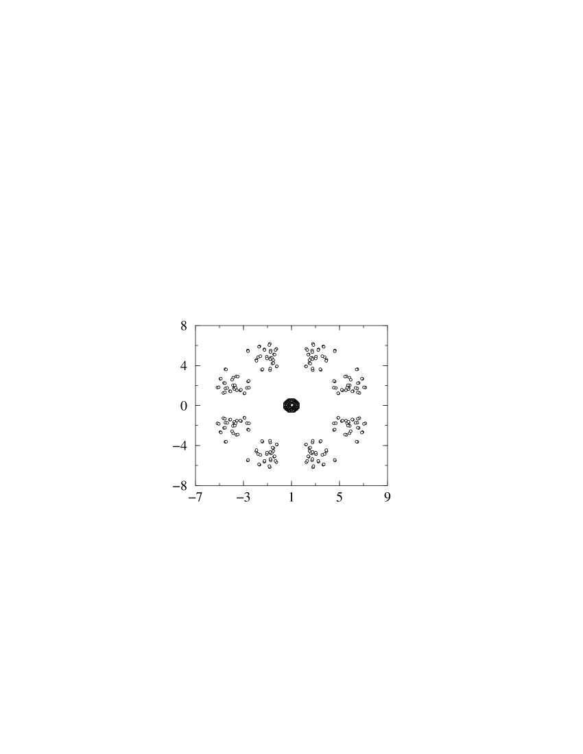
FIG. 1.: The spectrum of $\Lambda(x)$ in the complex plane on a $4\times 4\times 4$ lattice in SU(2) gauge group.

Then, for the representation of Eq.(12),

$$X_{i}=\sqrt{\frac{1}{r_{E}}}\Gamma_{i},\qquad Y_{i}=\sqrt{\frac{1}{r_{E}}}\Gamma_{D+i}+\Gamma_{2D+1},$$ (62)

we find

$$\Gamma=\Gamma_{2D+1}.$$ (63)

Since the eigenvalues of $\Lambda(x)$ always consist of complex conjugate pairs and degenerated ones on real axis, we conclude the determinant of our fermion matrix is positive in SU(2) gauge fields in any dimensions.

Now we show a numerical evidence. Fig.1 shows the spectrum of our fermion matrix in a typical background configuration of link variables for SU(2) gauge group in $(1+2)$ dimensions. We find that their distribution is symmetric with respect to the real axis as expected. Similarly in $(1+3)$ dimensions we can numerically confirm the symmetry with respect to the real axis, and the positivity of the determinant.

IV discussion and summary

In the previous paper [8] we reported analytical and numerical results on the fermion determinant of our new action in $(1+1)$ dimensions. In the case of U(1) gauge group, we were faced with the problem of convergence in numerical simulations. The cause of the poorness of the convergence is that the summation of the $\det(1-S_{0}^{\dagger}(x)U_{E}(x))=\det(1-e^{i\Theta}\tilde{S}_{0}^{\dagger}(x)U_{E}(x))$ over arbitrary phase angle $\Theta$ is canceled out accidentally. The element $e^{i\Theta}$ comes from the one sided time difference operator $S_{0}^{\dagger}(x)$ with $\theta_{0}(x)$ replaced by $\theta_{0}(x)+\Theta$, i.e. $S_{0}^{\dagger}(x)=e^{i\Theta}\tilde{S}_{0}^{\dagger}(x)$, where $\theta_{0}(x)$ is defined by $U_{x,x+\hat{0}}=e^{i\theta_{0}(x)}$ [8]. Therefore we must have control of the phase angle $\Theta$ in order to get good convergence in the $(1+1)$-dimensional U(1) gauge theory. In fact we analytically showed that our fermion determinant is real for all configurations and positive for most configurations under the T-condition ($\theta_{0}(x)=0$), which corresponds to the temporal gauge condition on the infinite lattice, or the GT-condition ($\sum_{x}\theta_{0}(x)=n\pi$ : $n=\mbox{even}$), which is achieved by a gauge transformation on the infinite lattice. It was also verified numerically. On the other hand we got good convergence without any conditions in $(1+1)$-dimensional SU(N) case, because the element like $e^{i\Theta}$ does not belong to the SU(N) group.

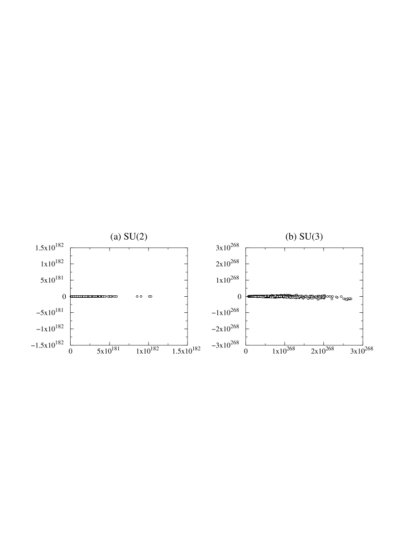
FIG. 2.: The distribution in the complex plane of our fermion determinants in a) SU(2) and b) SU(3) for each configurations of 2000 Monte Carlo iterations after getting good equilibrium, i.e. after 2000 iterations, on a $4\times 4\times 4$ lattice at $\beta=2.0$.

The above discussion is applicable to higher dimensions to a certain extent. In SU(2) group our fermion determinant is analytically shown real and positive in any dimensions. In Fig.2(a) we give the numerical evidence that the determinant is real and positive in $(1+2)$ dimensions. In the case of SU(3) group, we cannot prove the reality of the determinant. But from Fig.2(b) we see that the distribution of the determinant is concentrated near the real axis without any conditions and the phase angle of the determinant is small. We have obtained similar results in $(1+3)$ dimensions. When the phase angle of the fermion determinant is small enough, we can neglect the phase factor and make use of $|\det\Lambda(x)|$ instead of $\det\Lambda(x)$. In the above numerical simulations link variables are updated by the Metropolis method and determinants are calculated by the LU decomposition. So there are no systematic errors in the determinants.

In conclusion, we believe that our new fermionic action is a profitable formulation for the numerical simulations of SU(2) and SU(3) lattice gauge theory.

REFERENCES

[1] H. B. Nielsen and M. Ninomiya, Nucl. Phys. B185,
20 (1981); B193, 173 (1981).
[2] K. Wilson, Phys. Rev. D 10, 2445 (1974);
New Phenomena in Subnuclear Physics, edited by A. Zichichi
(Plenum, New York, 1977).
[3] L. Susskind, Phys. Rev. D 16, 3031 (1977).
[4] P. H. Ginsparg and K. G. Wilson, Phys. Rev. D 25,
2649 (1982).
[5] I. Horváth, Phys. Rev. Lett.
81, 4063 (1998);
W. Bietenholz, hep-lat/9901005.
[6] A. Hayashi, T. Hashimoto, M. Horibe,
and H. Yamamoto, Phys. Rev. D 55, 2987 (1997).
[7] M. Horibe, T. Hashimoto, A. Hayashi,
and H. Yamamoto, Phys. Rev. D 56, 6006 (1997).
[8] A. Takami, T. Hashimoto, M. Horibe
and A. Hayashi, hep-lat/0001011.