DESY 00-033

HLRZ2000_3

ON THE ETA-INVARIANT IN THE 4D CHIRAL U(1) THEORY


                   V. BORNYAKOV
                   Institute for High Energy Physics IHEP,
                   142284 Protvino, Russia

                   A. HOFERICHTER
                   Deutsches Elektronen-Synchrotron DESY and NIC,
                   15735 Zeuthen, Germany

                   G. SCHIERHOLZ
                   Deutsches Elektronen-Synchrotron DESY,
                   22603 Hamburg, Germany   and   
                   Deutsches Elektronen-Synchrotron DESY and NIC,
                   15735 Zeuthen, Germany

                   A. THIMM
                   Institut für Theoretische Physik, Freie Universität Berlin,
                   14195 Berlin, Germany

1 Introduction

In this talk we will focus on the imaginary part of the effective action of a four–dimensional chiral U(1) theory. Let us recall some relations in the continuum first, as they will be our guideline for the considerations on the lattice. Consider a compactified Euclidean space–time of four dimensions with chiral effective action $\,W[A]\,$ for a, say, left–handed fermion $\,\psi\,$ formally defined through

$${\rm e}^{-W[A]}=\int\!\!\!D\bar{\psi}D\psi\,{\rm e}^{-S[\bar{\psi},\,\psi,\,A]}\>.$$ (1)

The fermionic action $\,S[\bar{\psi},\psi,A]\,$ in the presence of an external gauge field $\,A_{\mu}=-A_{\mu}^{\dagger}\,$ is given by

$$S[\bar{\psi},\psi,A]=\int\!\!d^{4}x\>\bar{\psi}\not{D}_{L}[A]\psi\>,$$ (2)

with the usual definitions of the Dirac operator $\,\not{D}\,$ and the projectors $\,P_{R,L}$

$$\not{D}_{L}[A]=\not{D}[A]P_{L}\,,\quad\not{D}={\rm i}\gamma^{\mu}(\partial_{\mu}+A_{\mu})\,,\quad P_{R,L}=\frac{1}{2}(1\pm\gamma_{5})\;.$$ (3)

To make $\,W[A]\,$ better defined, one applies the doubling trick: $\,\not{D}_{L}[A]\,\rightarrow\,{\rm i}\not{\partial}P_{R}+\not{D}_{L}[A]$. Now, let $\,A_{t}=(1-t)A_{0}+tA\,,\;t\in[0,1],\,$ be a path connecting some initial configuration $\,A_{0}\,$ and $\,A\,$ in the same topological sector. Then, it is known by the work of [1] and others that

$${\rm Im}W[A]-{\rm Im}W[A_{0}]=\pi\eta+2\pi Q_{5}(A_{t})\,,$$ (4)

where $\,\eta=\eta[A]\,$ denotes the eta–invariant [2] of the associated five–dimensional Dirac operator $\,\mathbb{H}={\rm i}\gamma_{5}\partial_{t}+\not{D}[A_{t}]\,$ and $\,Q_{5}(A_{t})$ is the Chern-Simons form. While $\,\eta\,$ is gauge invariant, $\,Q_{5}\,$ encodes the anomaly $\,\delta_{g}W[A]\propto{\rm i}\,\delta_{g}Q_{5}$, where $\,\delta_{g}\,$ is the variation w.r.t. a gauge transformation $\,g$. On the other hand, the real part of the effective action is basically vector–like. Denoting the effective action of the associated vector theory by $\,W_{V}$, it is known that

$${\rm Re}W[A]-{\rm Re}W[A_{0}]=\frac{1}{2}\Big{(}W_{\rm V}[A]-W_{\rm V}[A_{0}]\Big{)}\,,$$ (5)

up to local counterterms. Thus, in the anomaly free model (i.e., $\,Q_{5}=0$) the eta–invariant represents the chiral nature of the theory. Hence, from the point of view of a practical implementation of a chiral gauge theory on the lattice, it is most desirable to have the imaginary part of the chiral effective action under control. Some cases, in which the path integral can be evaluated on the lattice are listed below.

• One has analytic knowledge of the eta–invariant as some expression in the gauge fields, which can be managed in lattice computations.

• The eta–invariant is small but not zero: $\eta\,\sim\,0$.

  In this case, one can include the effect of $\,\eta\,$ by re-weighting the observables $\,{\cal O}\,$ by $\langle{\cal O}\rangle=\langle\,{\cal O}\,{\rm e}^{i\pi{\eta}}\,\rangle_{ReW}/\langle\,{\rm e}^{i\pi{\eta}}\,\rangle_{ReW}\,,\>$ where $\,\langle\>\cdot\>\rangle_{ReW}\,$ means averaging w.r.t. the vector–like real part of $\,W$, only.

• The eta–invariant vanishes after anomaly cancellation: $\eta\,=\,0$.

  Consequently, the measure is purely vector–like, no re-weighting as in (b) is necessary.

The initial goal of our investigation is to determine, which of the cases applies to our chiral U(1) model. Although there has been enormous progress on the conceptual side of chiral gauge theories on the lattice, e.g.[4], the details, even in the ‘simplest’ four–dimensional model, can be quite involved.

2 Chiral U(1) Theory on the Lattice

The lattice fermionic action $\,S_{F}\,$ under consideration is given by

$${S_{F}}[{\bar{\psi}},\psi,U]=\,{\bar{\psi}}\,{\bf\mathbb{M}}[U]\,\psi\,,$$

where $\,U\,$ is an external lattice gauge field with (compact) link variables $U_{\mu}(x)\in\,{\rm U(1)}$. The fermion matrix $\,\mathbb{M}[U]={\not{\mathbb{D}}}[U]+\mathbb{W}[U]\,,$ has Dirac part

$$\not{\mathbb{D}}=\not{D}P_{R}+\not{D}P_{L} = \left(\begin{array}[]{cc}0&{D}_{{L}\,\;~{}}\\ {D}_{{R}\;\,~{}}&0\\ \end{array}\right)$$ (8)

and Wilson term

$$\mathbb{W} = \left(\begin{array}[]{cc}W_{{L}{R}}&0\\ 0&W_{{R}{L}}\\ \end{array}\right)\,.$$ (11)

We used the so-called ungauged Wilson term

$$\mathbb{W} = -\frac{1}{2}\left(\begin{array}[]{cc}\partial^{b}\partial^{f}&0\\ 0&\partial^{f}\partial^{b}\\ \end{array}\right)\,,$$ (14)

where $\partial^{f,b}\,$ denotes the lattice forward and backward derivative, respectively. In this case there are no counterterms for the imaginary part of the effective action [5].

In our four–dimensional chiral model, we have chosen the right-handed component of the gauge field $U_{R}$ to be trivial, in such a way that $\,{D}_{R}\,\rightarrow\,{\partial}_{R}$.

We evaluate the imaginary part of the fermionic effective action,

$${\rm Im}\,W=-{\rm Im}\,(\ln\det\mathbb{M}\,)\,,$$

in the continuum fermion approach. For details we refer to the literature (e.g.[5]–[9]). The basic idea is to associate bosonic and fermionic degrees of freedom to different cutoffs $\,a^{-1}\,$ and $\,a_{f}^{-1}\,$, respectively. Here $\,a\,$ denotes the lattice spacing of the original lattice, where the original lattice gauge field $\,U^{a}\,$ resides, and $\,a_{f}<a\,$ is the lattice spacing of a finer lattice which ‘carries’ the fermions, in the background of some gauge field $\,U^{a_{f}}\,$ obtained by suitable interpolation (e.g. [10]) from $\,U^{a}$. To evaluate the fermionic effective action for the continuum fermions we have to consider

$$-\lim_{a_{f}\to 0}\,\Big{(}\,\ln\det\mathbb{M}[U^{a_{f}}]\,\Big{)}\,,$$ (15)

with $\,a\,$ held fixed. Eventually, also the limit $\,a\rightarrow 0\,$ has to be taken, which we will not perform here, since it is not necessary for meeting the initial goal. For perturbative fields, it has been shown that (15) exists and has correct properties after adding the appropriate counterterms, e.g. [9]. Gauge invariance breaking effects vanish as $\,O(a_{f}/a)\,$ [5, 8].

To compute $\>\det\mathbb{M}[U^{a_{f}}]\>$ we apply a non-Hermitean Lanczos procedure with complete re-orthogonalization. In an additional step we construct the anomaly free model by imposing the anomaly cancellation condition:

$$\sum_{\alpha=1}^{N_{f}}\epsilon_{\alpha}c_{\alpha}^{3}=0\,.$$ (16)

The sum runs over the $\,N_{f}\,$ different flavors with chiralities $\,\epsilon_{\alpha}\,$ and fermion charges $\,c_{\alpha}$. In the anomaly free case, we formally define a lattice eta–invariant by

$$\lim_{a_{f}\to 0}\,{\rm Im}W[U^{a_{f}}]\,\stackrel{{\scriptstyle!}}{{=}}\,\pi\eta\,;\quad{a={\rm const}}\,,$$

where we have utilized the continuum relations.

3 Perturbative Structure

Before turning to numerical results, we will investigate the perturbative structure of the imaginary part of the effective action.

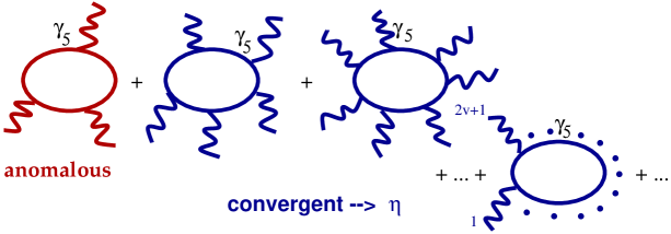
Figure 1: Graphical representation of $\,{\rm Im}W[A]$.

For simplicity, we will stick to continuum relations, as in the introduction. Fig. 1 represents $\,{\rm Im}W[A]\,$ in terms of graphs, with external field $\,A$. In our case of four dimensions just the first diagram is divergent, while the others are convergent and (up to a factor) sum up to $\,\eta[A]$. Hence, after anomaly cancellation, the five–leg diagram is expected to give the leading contribution to $\,{\rm Im}W[A]\,$ for perturbative fields. Just this diagram would require the investigation of $\,O(10000)\,$ terms in the general case. Therefore, we will choose another strategy to probe the perturbative behavior. By using plane-wave configurations

$$A_{\mu}(x)=c_{\alpha}\,\sum_{l}\,{a}_{\mu,{l}}\cos(k_{l}x)+{b}_{\mu,l}\sin(k_{l}x)$$ (17)

as numerical input, we rescale the charge $\,c_{\alpha}\,\rightarrow\,\xi\,c_{\alpha}$, keeping all other parameters fixed, and set the corresponding effective actions into relation. For small enough amplitudes and charges, we expect for one flavor $\alpha$

$$\frac{{\rm Im}W_{[\xi\,c_{\alpha}]}}{{\rm Im}W_{[c_{\alpha}]}}\;\sim\;\xi^{2\nu+1}\>,$$ (18)

where $\,(2\nu+1)\,$ is the number of external legs of the first non-vanishing diagram in Fig. 1 and $\,W_{[c_{\alpha}]}\,$ is the effective action for the given charge $\,c_{\alpha}$. With $\,\xi=2\,$ in (18) typical numbers like $\,2^{3}\,$ or $\,2^{5}\,$ would single out the anomalous or the five–leg diagram as leading contribution to $\,{\rm Im}W$, respectively.

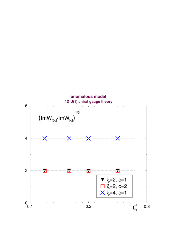
Figure 2: The $\,a_{f}$ dependence of (the cubic root of) eq.(18) for different scaling factors $\,\xi$ and charges $\,c$. The dashed lines indicate the expectation according to the anomalous three-leg graph.

Indeed, we find this characteristic behavior as shown in Figs. 2, 3, where we display the $\,\xi\,$ and $\,a_{f}\,$ dependence of eq.(18). The dashed lines represent the behavior predicted by the anomalous diagram (i.e. $\,\nu=1\,$ in Fig. 2) and, after anomaly cancellation, the five–leg diagram (i.e. $\,\nu=2\,$ in Fig. 3). In this way, we nicely reproduce the perturbative structure of $\,{\rm Im}W$. In general, the imaginary part of the effective action does not vanish, but for typical configurations at weak coupling it might have a small magnitude, such that still the case (b), or in some approximation, (a) listed in the introduction is realized.

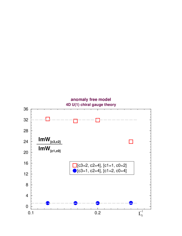
Figure 3: The $\,a_{f}$ dependence of eq.(18) for the same external gauge fields as in Fig. 2, but after anomaly cancellation. $c_{\rm odd(even)}\,$ denote the charges of the left(right)–handed fermions involved, according to (16): for instance, $\>[c_{1}\!=\!1,\,c_{0}\!=\!2]\,$ is a shorthand notation for the anomaly free $(11111111\>2)$ model. The dashed lines indicate the behavior expected from the five–leg diagram.

4 Numerical Results

Here we consider the case of weak coupling configurations, without any topological obstructions (e.g. DeGrand–Toussaint monopoles). We investigated four gauge configurations, denoted by $\,U_{1},\dots,U_{4}\,$ residing on an original lattice of size $\,3^{4}$ and which were interpolated to finer lattices up to $\,L_{f}=8$. The interpolation has been refined in order to estimate lattice errors. Details have been presented in [13].

The configurations $\,U_{1},\,U_{2},\,U_{3}\,$ were generated randomly with the constraint that the link angles $\,|\,\theta_{\mu}(x)\,|<\pi/5,\,\pi/6,\,\pi/8\,$.   $U_{4}\,$ was generated at weak coupling in a (quenched) vector theory simulation. All original configurations were free of Dirac plaquettes and monopoles. The plaquette values on the original lattice are given in Tab. 1.

	$U_{1}$	$U_{2}$	$U_{3}$	$U_{4}$
$1\!-\!\cos\theta_{P}$ :	0.251	0.169	0.098	0.0062

Table 1: Plaquette values of the original configurations $\,U_{1},\dots,\,U_{4}$.

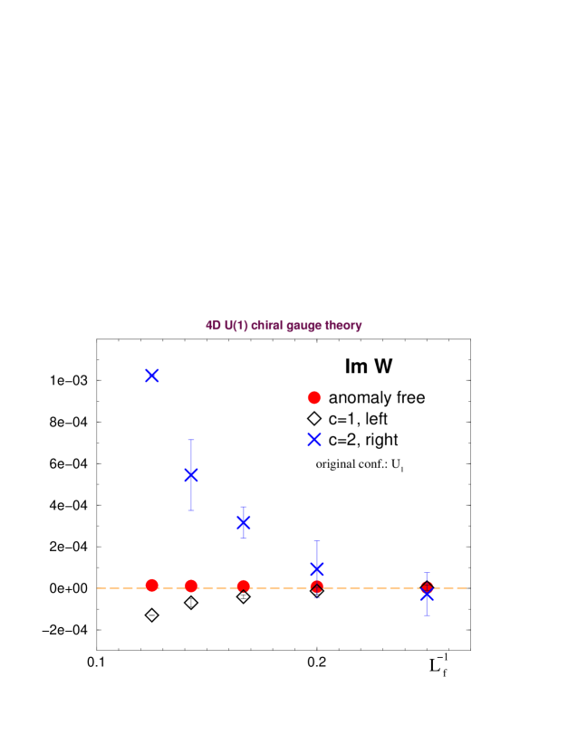
Figure 4: ${\rm Im}W\,$ vs. $\,L_{f}^{-1}\,$ for the configuration $\,U_{1}\,$ with different charges and chiralities.

In Fig. 4 we display the $\,a_{f}\,$ dependence of $\,{\rm Im}W\,$ for the configuration $\,U_{1}$. The error bars in the figure should not be confused with Monte Carlo errors – they are an estimation of lattice errors, provided by the interpolation procedure. Since the anomaly is canceled event by event, the error bars can be small in the anomaly free case, although lattice errors are quite visible in the anomalous charge two–case. Fig. 5 shows the results for the original configuration $\,U_{4}$. For configurations $\,U_{2,3}$ we find similar behavior and the magnitudes of $\,{\rm Im}W\,$ are in between the cases of Fig. 4 and Fig. 5. Despite a clear signal before anomaly cancellation, the imaginary part of the effective action remains close to zero in the anomaly free model. We find a difference of up to two orders in magnitude for $\,{\rm Im}W\,$ between the models with and without anomaly.

5 Summary

In general, the imaginary part of the effective action does not vanish in the investigated model, as can be shown by perturbative analysis. However, for the given configurations, which we have chosen to mimic typical configurations in the weak coupling region, we find that $\,{\rm Im}W\,$ basically consists of the anomaly. After anomaly cancellation we have at most $\,|\,{\rm Im}W\,|\,<\,1.5\cdot 10^{-5}$. This implies a very small value of $\,\eta$, even though it may take any value in the range $[-1,\,1)$. For weak fields, our investigation favors options (a), (b) as listed in the introduction. Where option (a) would involve the evaluation of a few (convergent) diagrams of Fig. 1 by lattice techniques.

6 Acknowledgments

This work has been partially supported by the INTAS 96-370 grant. V.B. acknowledges support from RFBR 99-01230a grant. The calculations have been partly done on the T3E at ZIB and we thank H. Stüben for technical support. Thanks go to K. Jansen, B. Andreas and K. Scharnhorst for fruitful discussions.

We would like to thank all the organizers, in particular V. Mitrjushkin, for the warm atmosphere and a wonderful workshop in Dubna.

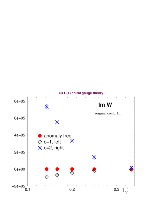
Figure 5: As Fig. 4, but for the configuration $\,U_{4}$.

References

- [1] Alvarez-Gaumé, L., Della Pietra, S., Della Pietra, V., Phys. Lett. 166B, 177 (1986).
- [2] M.F. Atiyah, V.K. Patodi, I.M. Singer, Math. Proc. Camb. Phil. Soc. 77, 43 (1975).
- [3] T. Aoyama, Y. Kikukawa, hep-lat/9905003.
-
[4]
M. Lüscher, Nucl. Phys.B549, 295 (1999); hep-lat/9909150;
H. Neuberger, hep-lat/9912020; hep-lat/9909042; and this volume. - [5] G.T. Bodwin, Phys. Rev. D54, 6497 (1996).
- [6] M. Göckeler, G. Schierholz, Nucl. Phys. B (Proc. Suppl.) 29B,C, 114 (1992).
- [7] G. ’t Hooft, Phys. Lett. B349, 491 (1995).
- [8] P. Hernández, R. Sundrum, Nucl. Phys. B455, 287 (1995).
- [9] V. Bornyakov, G. Schierholz, A. Thimm, Prog. Theor. Phys. Suppl. 131, 337 (1998).
- [10] M. Göckeler, A.S. Kronfeld, G. Schierholz, U.-J. Wiese, Nucl. Phys. B404, 287 (1993).
- [11] H. Suzuki, hep-lat/9911009.
- [12] V. Bornyakov, A. Hoferichter, G. Schierholz, A. Thimm, hep-lat/9909135.
- [13] A. Thimm, talk at this conference and at Lattice’99.