CORE and the Haldane Conjecture

Marvin Weinstein

Stanford Linear Accelerator Center

Stanford University, Stanford, California 94309

ABSTRACT

The Contractor Renormalization group formalism (CORE) is a real-space renormalization group method which is the Hamiltonian analogue of the Wilson exact renormalization group equations. In an earlier paper[3] I showed that the Contractor Renormalization group (CORE) method could be used to map a theory of free quarks, and quarks interacting with gluons, into a generalized frustrated Heisenberg antiferromagnet (HAF) and proposed using CORE methods to study these theories. Since generalizations of HAF’s exhibit all sorts of subtle behavior which, from a continuum point of view, are related to topological properties of the theory, it is important to know that CORE can be used to extract this physics. In this paper I show that despite the folklore which asserts that all real-space renormalization group schemes are necessarily inaccurate, simple Contractor Renormalization group (CORE) computations can give highly accurate results even if one only keeps a small number of states per block and a few terms in the cluster expansion. In addition I argue that even very simple CORE computations give a much better qualitative understanding of the physics than naive renormalization group methods. In particular I show that the simplest CORE computation yields a first principles understanding of how the famous Haldane conjecture works for the case of the spin-$1/2$ and spin-$1$ HAF.

Submitted to Physical Review D.

1 Introduction

The Contractor Renormalization group (CORE) formalism is a Hamiltonian analogue of the Wilson exact renormalization group equations for systems defined by a path integral. Although it is a real-space renormalization group method it differs from earlier naive real-space renormalization group methods[1], or more accurate methods such as the density-matrix renormalization group approach of S. R. White[2], in that it is in principle exact, is amenable to evaluation by a convergent non-perturbative approximation procedure and finite range results are easily improved by a simple extrapolation technique. In addition, the great flexibility one has in the choice of truncation procedure allows one to apply CORE to problems in ways which are impossible with other methods. In particular, CORE can be used to produce a non-trivial renormalization group analysis of a lattice gauge-theories truncated to totally gauge-invariant block states, something which is impossible in the either naive real-space or the density matrix renormalization group approach.

In an earlier paper[3] I showed that CORE can be used to map a theory of free quarks, and quarks interacting with gluons, into a generalized frustrated Heisenberg antiferromagnet (HAF) and proposed using the same CORE methods to study these theories. Since generalizations of HAF’s exhibit all sorts of subtle behavior which from a continuum point of view, are related to topological properties of the theory, it is important to know that CORE can be used to extract this physics. Moreover, since the really interesting cases are Hamiltonian theories in 3-spatial dimensions, it is important that CORE be able to produce qualitatively and quantitatively correct pictures of the low energy physics of these theories with truncation schemes that keep only a few states per block and only a few terms in the cluster expansion. The purpose of this paper is to show that, unlike the original naive real-space renormalization group methods, relatively simple CORE computations based upon keeping a small number of states per block and only a few terms in the finite range cluster expansion give accurate results which can be systematically improved. It is the fact that one can achieve reasonable accuracy keeping only a few states per block which makes it possible to apply CORE to Hamiltonian theories defined on two and three dimensional lattices.

A detailed discussion of the application of CORE to the Hamiltonian version of the 1+1-dimensional Ising model, which was presented in an earlier paper[4], showed that one could achieve highly accurate results for the groundstate energy density, magnetization and mass-gap with a scheme which kept only two states per three-site block and only up to range-3 terms in the cluster expansion (which means that the biggest problem one has to deal with is a nine-site sublattice). The same paper also presented, among other things, a brief discussion of the method as applied to the spin-1/2 HAF. Since the purpose of that discussion was to use the example to explain certain features of the CORE method I didn’t include any remarks about how the method compares to the naive renormalization group scheme or how to obtain higher accuracy results. These issues will be addressed in this paper before moving on to the issue of what is different about the spin-1 case and how it relates to Haldane’s conjecture[7]. My purpose in discussing the spin-1 HAF, is to show that, unlike the naive renormalization group approach, a simple 4-state range-2 CORE computation for the spin-1 HAF, is good enough to provide a straightfoward understanding of the physics. This simple calculation shows that the physics of the spin-1 model is intimately related to the structure of a more general theory with Hamiltonian $H=\sum_{i}[\vec{s}(i)\cdot\vec{s}(i+1)-\beta\,(\vec{s}(i)\cdot\vec{s}(i+1))^{2}]$ which has a valence bond ground state when $\beta=-1/3$. In a naive renormalization of the same theory the term $-\beta\,(\vec{s}(i)\cdot\vec{s}(i+1))^{2}]$ will not appear and thus, the naive renormalization group approach will not see any difference between the spin-1/2 theory and the spin-1 theories.

2 The Basic Problem

The generic real-space renormalization group (RSRG) method consists of three steps. First one divides the lattice into blocks, each of which contains a finite number of sites. Next one restricts the full Hamiltonian to just those terms which relate to a single block, diagonalizes it, selects a finite subset of its lowest energy eigenstates and then uses them to generate a subspace of the full Hilbert space which we will refer to as the set of retained states. Finally, one constructs a new renormalized Hamiltonian which acts with the space of retained states and which has the same low-energy physics as the full theory. Of course, the details of how to choose blocks, how to construct the appropriate block Hamiltonian and how to construct the renormalized Hamiltonian acting on the space of retained states differs from method to method.

2.1 The Naive Real-Space Renormalization Group

The naive real-space renormalization group method implements the RSRG procedure in a straightforward manner and is basically a version of the Rayleigh-Ritz variational calculation familiar from elementary quantum mechanics. In order to understand the motivation behind the method and its limitations consider the example of a simple spin-1/2 Heisenberg anti-ferromagnet with the Hamiltonian

$$H=\sum_{j=-\infty}^{\infty}\vec{s}(j)\cdot\vec{s}(j+1).$$ (1)

Begin by dividing the lattice into disjoint blocks each containing three sites, $B_{j}=\{3j,3j+1,3j+2\}$ and define the block Hamiltonian

$$H_{B_{j}}=\vec{s}(3j)\cdot\vec{s}(3j+1)+\vec{s}(3j+1)\cdot\vec{s}(3j+2)$$ (2)

Next diagonalize the block Hamiltonian and keep its two lowest lying states. This is a simple exercise since the block Hamiltonian can be rewritten in terms of the total block spin operator $\vec{S}_{\rm TOT}(3j,3j+1,3j+2)=\vec{s}(3j)+\vec{s}(3j+1)+\vec{s}(3j+2)$ and the operator $\vec{S}_{\rm TOT}(3j,3j+2)=\vec{s}(3j)+\vec{s}(3j+2)$, as

$$H_{B_{j}} = \vec{s}(3j)\cdot\vec{s}(3j+1)+\vec{s}(3j+1)\cdot\vec{s}(3j+2)$$ (3)

$$= \vec{s}(3j+1)\cdot\left(\vec{s}(3j)+\vec{s}(3j+2)\right)$$ (4)

$$= \frac{1}{2}\left(S^{2}_{\rm TOT}(3j,3j+1,3j+2)-S^{2}_{\rm TOT}(3j,3j+2)-\frac{3}{4}\right)$$ (5)

The Hilbert space for the three-site problem is a product of three spin-1/2 states and since $H_{B_{j}}$ is rotationally invariant its eigenstates decompose into the direct sum of a spin-3/2 multiplet and two spin-1/2 multiplets. From Eq. 3 we see that the lowest lying multiplet is the spin-$1/2$ multiplet obtained by coupling the spin on site $3j+1$ to the spin-1 multiplet made out of the product of the spins on sites $3j$ and $3j+2$. Thus, keeping the two lowest lying states amounts to keeping the lowest lying spin-1/2 multiplet. We then use these states to generate the subspace of retained states.

The intuition behind the final step in the naive real-space renormalization group method, constructing the renormalized Hamiltonian, is based upon the observation that the gaps between the one block multiplets are fairly large. One guesses that a reasonable variational wavefunction for the true groundstate of the system can be constructed within the space of retained states; i.e., the set generated by taking all possible tensor products of the two lowest lying spin-1/2 states per block. A variational calculation based upon this assumption says that solving for the best variational state is equivalent to diagonalizing the Hamiltonian obtained by computing all matrix elements of the original Hamiltonian in the space of retained states. To be specific, consider the three-site blocking scheme proposed above. Let us denote by $W_{j}$ the lowest lying spin-1/2 multiplet for block $B_{j}$ and define the space of retained states as

$$W=\bigotimes_{j}W_{j},$$ (6)

Then, if we let $P_{W}$ denote the projection operator onto the space of retained states the renormalized Hamiltonian is

$$H^{\rm ren}=P_{W}HP_{W}.$$ (7)

To explicitly compute $H^{\rm ren}$ it is convenient to rewrite the full Hamiltonian as a sum of two terms; i.e.

$$H=\sum_{j}H_{B_{j}}+\sum_{j}H_{B_{j}B_{j+1}}\\$$ (8)

where $H_{B_{j}}$ is the block Hamiltonian defined in Eq. 3 and $H_{B_{j}B_{j+1}}$ is the block-block coupling term

$$H_{B_{j}B_{j+1}}=\vec{s}(3j+2)\cdot\vec{s}(3(j+1)).$$ (9)

Since the space of retained states is constructed of tensor products of eigenstates of the $H_{B_{j}}$ which all have the eigenvalue $-1$, it is clear that

$$P_{W}H_{B_{j}}P_{W}=-{\bf 1}_{j},$$ (10)

and so the first sum of terms in Eq. 8 gives a contribution of $-1$ for each three-site block $B_{j}$, or in other words, a contribution of $-1/3$ to the energy density of the groundstate.

The block-block interaction term is a sum of terms, each of which touches two adjacent blocks, so to compute $P_{W}H_{B_{j}B_{j+1}}P_{W}$ we only need to compute the matrix elements of $\vec{s}(3j+1)$ and $\vec{s}(3(j+1))$ between the states in the lowest lying spin-1/2 multiplet of the three-site problem. This is easily done and the result is that the truncated operators on the first and last sites of a three-site block are proportional to the spin-1/2 generators with a proportionality factor of $2/3$; i.e.,

$$P_{W_{j}}\vec{s}(3j+1)P_{W_{j}}=P_{W_{j}}\vec{s}(3j)P_{W_{j}}=\frac{2}{3}\vec{s}(j),$$ (11)

where $\vec{s}(j)$ now stands for the usual spin operators acting on the spin-1/2 representation associated with each site of the new lattice. Combining these facts we obtain a renormalized Hamiltonian

$$H^{\rm ren}=\sum_{j}(-{\bf 1}_{j})+\frac{4}{9}\vec{s}(j)\cdot\vec{s}(j+1)$$ (12)

where $H^{\rm ren}$ is to be thought of as acting on a the states of a thinner lattice (one with one-third as many sites) with a spin-1/2 degree of freedom associated with each site, $j$. Note that I have chosen to include the energy density as a sum of single-site operators which have a coefficient of $-1$ and which happen to be the single-site identity operator.

From Eq. 12 we see that the Hamiltonian reproduces itself up to an additive $c$-number and a multiplicative factor of $4/9$. It follows immediately that if we repeatedly apply the same naive renormalization group transformation group, then after $n$ steps the renormalized Hamiltonian will have the same form; i.e., a $c$-number term which gives the vacuum energy and an interaction term which is multiplied by a factor $(4/9)^{n}$

$$H^{\rm ren}_{n}=C_{n}\sum_{j}{\bf 1}_{j}+(4/9)^{n}\sum_{j}\vec{s}(j)\cdot\vec{s}(j+1)$$ (13)

where the coefficients $C_{n}$ satisfy the recursion relation

$$C_{n+1}=3C_{n}-(4/9)^{n}$$ (14)

The first term on the right hand side of this equation comes from the fact that the term proportional to the unit matrix contributes $3C_{n}$ to the energy of every state in the three-site Hamiltonian and the second term is just the fact that the lowest lying spin-1/2 multiplet for the three-site problem has energy $-1$ times the scale factor of the $\vec{s}\cdot\vec{s}$ term. To extract the groundstate energy density we observer that after $n$-steps each site on the new lattice has is equivalent to $3^{n}$ sites on the old lattice, thus the energy density is

$${\cal E}=\lim_{n\rightarrow\infty}{\cal E}_{n}=\lim_{n\rightarrow\infty}\frac{C_{n}}{3^{n}}$$ (15)

where

$${\cal E}_{n+1}=\frac{C_{n+1}}{3^{n+1}}={\cal E}_{n}-\frac{1}{3}(4/27)^{n}$$ (16)

and ${\cal E}_{1}=-1/3$. Clearly, one can derive a recursion relation for the ${\cal E}_{n}$’s and sum the resulting geometric series to get the groundstate energy density

$${\cal E}=\frac{-1}{3(1-4/27)}=-0.3913;$$ (17)

which is to be compared to the exact answer of $-.4431$. This corresponds to a fractional error of $12\%$. Furthermore, from the fact that the coefficient in front of the interaction term $\vec{s}(j)\cdot\vec{s}(j+1)$ tends to zero as $n\rightarrow\infty$ we see that the theory has to be massless.

Although the computation of the groundstate energy density is only good to $12\%$, (which is not as good as the Anderson spin-wave computation which is accurate to about $2\%$) it is very simple and one might hope that it can be easily improved upon. Unfortunately, this is not as easy as it sounds.

An obvious way to try and improve the calculation is to work with larger blocks and keep a larger number of states per block so as to get a larger space of retained states and the possibility of a better variational wavefunction. Appealing as this sounds, the brute force approach of keeping more of the lowest lying eigenstates doesn’t provide a rapid improvement of the results obtained in the simplest two state approach. The problem is that when the block is larger the wavefunctions of the lowest lying states develop nodes at the walls of the block and therefore the block-block recoupling terms come out smaller than they should be in the renormalization group step. If one is going to work with larger blocks and keep more states one has to be clever about choosing the states to keep. This is what is done in the density matrix renormalization group approach. The principle shortcomings of the density matrix approach is that in general, in order to achieve high accuracy, one has to keep a large number of states per block which means: first, that the method is purely numerical in character and one loses contact with the original structure of the Hamiltonian; second, that the method is really best suited to Hamiltonian theories on a one-dimensional spatial lattice since the number of states per block which must be kept to guarantee the correct recoupling across the boundary of the block in higher dimensions grows quickly and the problem becomes computationally difficult; third, for the case of a lattice gauge-theory, one cannot adopt a truncation scheme which keeps only locally gauge-invariant states, as the density matrix method will intrinsically require keeping states in which flux leaves through the boundaries of a block. This inability to work with locally color-singlet states makes using the density matrix method unwieldy for extracting the low energy physics of a theory like lattice QCD.

CORE takes a different approach to getting improved results. It is based upon a formula which, given a truncation scheme for selecting the space of retained states, maps the original Hamiltonian to one which acts only on the space of retained states and this new Hamiltonian is guaranteed to have the same low energy physics as the original theory. Although CORE is based upon a scheme which, like the naive renormalization group approach, keeps only a small number of states per block, a CORE transformation generates new operators. Thus, one trades in the information carried by the extra states for extra operators in the renormalized Hamiltonian. The advantage of the CORE approach is that, as we will see, the number of extra operators which must be kept is much smaller than the number of extra states needed for a density matrix renormalization group calculation. Since the CORE method preserves the basic structure of the original theory the semi-analytic nature of the resulting renormalization group flow reveals what is happening in a more transparent manner. Moreover, as was discussed in Ref.[3], CORE allows one to study a theory such as lattice QCD by defining the space of retained states to be that generated by taking tensor products of local color singlet states.

2.2 CORE – The Basic Algorithm

CORE has two parts. The first is a theorem which defines the Hamiltonian analog of Wilson’s exact renormalization group transformation; the second is a set of approximation procedures which render nonperturbative calculation of the renormalized Hamiltonian doable. A detailed review of the general method can be found in Ref. [3] and a detailed presentation of the CORE formalism can be found in Ref. [4]. In this section I limit myself to a review of the basic concepts for the special case of a general Heisenberg antiferromagnet.

As in the case of the naive renormalization group, CORE defines the space of retained states as the image of a projection operator, $P$, acting on the original space, ${\cal H}$; i.e., ${\cal H}_{\rm ret}=P{\cal H}$. In what follows, for both the spin-$1/2$ and spin-$1$ case, this set of retained states will be defined by diagonalizing the Hamiltonian restricted to either a two or three-site block and defining $P$ as the operator which projects onto the subspace spanned by a small number of its lowest energy eigenstates.

The formula relating the original Hamiltonian, $H$, to the renormalized Hamiltonian having the same low energy physics is

$$H^{\rm ren}=\lim_{t\rightarrow\infty}[[T(t)^{2}]]^{-1/2}\,[[T(t)HT(t)]]\,[[T(t)^{2}]]^{-1/2},$$ (18)

where $T(t)=e^{-tH}$ and where $[[O]]=POP$ for any operator $O$ which acts on ${\cal H}$. It is worth noting that the $t=0$ version of Eq. 18 is just the definition of the naive renormalization group transformation.

While it is not generally possible to evaluate Eq. 18 exactly, it is possible to nonperturbatively approximate the infinite lattice version of $H^{\rm ren}$ to any desired accuracy. This is because $H^{\rm ren}$, as defined in Eq. 18, is an extensive operator and has the general form

$$H^{\rm ren}=\sum_{j}\sum_{r=1}^{\infty}h^{\rm conn}(j,r)$$ (19)

where each term, $h^{\rm conn}(j,r)$, stands for a set of range-$r$ connected operators based at site $j$, all of which can be evaluated to high accuracy using finite size lattices. Typically it isn’t necessary to calculate all the terms in $H^{\rm ren}$. Often one can obtain highly accurate results, or qualitatively correct results, by approximating $H^{\rm ren}$ by its range-2 or range-3 terms.

In general the range-1 connected term in the renormalized Hamiltonian is defined to be the matrix obtained by evaluating the $j^{\rm th}$ block Hamiltonian in the set of retained eigenstates,

$$h^{\rm conn}(j,1)=[[H_{\rm block}(j)]].$$ (20)

The range-2 part of the renormalized Hamiltonian is evaluated as follows: first, restrict the full Hamiltonian to two adjacent (i.e., connected) blocks and define the two-block retained states as tensor products of the single block retained states; next, use these states to define a projection operator and evaluate Eq. 18, where $H=H(j,j+1)$ is the Hamiltonian restricted to blocks $B_{j}$ and $B_{j+1}$ to obtain

$$H_{2-block}(j,j+1)=\lim_{t\rightarrow\infty}[[T(t)^{2}]]^{-1/2}\,[[T(t)HT(t)]]\,[[T(t)^{2}]]^{-1/2};$$ (21)

finally, construct the connected range-2 contribution to the renormalized Hamiltonian by subtracting the two ways of embedding the one-block computation into the connected two-block computation as follows,

$$h^{\rm conn}(j,2)=H_{2-block}(j,j+1)-h^{\rm conn}(j,1)-h^{\rm conn}(j+1,1).$$ (22)

It might appear to be difficult to take the $t\rightarrow\infty$ limit of Eq. 21, however it is easy to show that this limit can be evaluated as a product of the form

$$H_{2-block}(j,j+1)=R\,H_{\rm diag}\,R^{{\dagger}}$$ (23)

where $R$ is an orthogonal transformation and $H_{\rm diag}$ is a diagonal matrix. $H_{\rm diag}$ is constructed by expanding the image under $R$ of each of the tensor product states in a complete set of eigenstates of the two-block problem and putting the energy of the lowest lying eigenstate appearing in the expansion of each rotated state on the diagonal. $R$ is constructed to guarantee that for each rotated state, the lowest energy eigenstate of the two-block problem which appears in its expansion in a complete set of eigenstates is distinct from that appearing in the expansion of the other rotated states. As we will see in a moment, given the symmetries of the problem, constructing $R$ is straightforward for both the spin-$1/2$ and spin-$1$ HAF.

The generic range-$r$ connected contribution is obtained by evaluating

$$H_{r-block}(j,j+1,\ldots,j+r-1)=\lim_{t\rightarrow\infty}[[T(t)^{2}]]^{-1/2}\,[[T(t)HT(t)]]\,[[T(t)^{2}]]^{-1/2};$$ (24)

for the Hamiltonian restricted to a set of $r$-adjacent blocks. Finally, the connected range-$r$ contribution to the renormalized Hamiltonian is then defined as

$$h^{\rm conn}(j,r) = H_{r-block}(j,j+1,\ldots,j+r-1)-\sum_{m=0}^{1}h^{\rm conn}(j+m,r-1)$$ (25)

$$\ldots -\sum_{m=0}^{p}h^{\rm conn}(j+m,r-p)\ldots-\sum_{m=0}^{r-1}h^{\rm conn}(j+m,1).$$

3 Generalized Heisenberg Antiferromagnets

The general CORE method is extremely flexible since one has a great deal of freedom in choosing how to truncate the space of states. Once one commits to a given truncation algorithm, however, everything is specified and it only remains to choose how many terms one will compute in the cluster expansion. Given these two somewhat independent choices it is interesting to explore the way in which changing the truncation algorithm and changing the range of the cluster expansion affects the accuracy of the results obtained. The next section discusses this issue for the case of the spin-1/2 Heisenberg antiferromagnet. In order to explore the rate of convergence of the cluster expansion I will first discuss the extreme case of a single state truncation algorithm computed to range-$6$ in the cluster expansion and then I discuss the simplest two-state truncation algorithm computed to range-$4$ in the cluster expansion. In addition I will discuss the use of type two Padé approximants to extrapolate the resulting series for the groundstate energy density in the single state and two state situation.

3.1 CORE and the Spin-$1/2$ HAF: One State Truncation

As in the discussion of the naive renormalization group algorithm for the HAF we begin with the spin-1/2 Hamiltonian

$$H=\sum_{j=-\infty}^{\infty}\vec{s}_{j}\cdot\vec{s}_{j+1}$$ (26)

but, this time we consider various blocking and truncation algorithms. Before diving in to the computation it is worth explaining why we didn’t consider a two-site blocking procedure in our discussion of the naive renormalization group method. The reason becomes obvious if we rewrite the two-site Hamiltonian, as

$$H_{\rm block} = \vec{s}_{1}\cdot\vec{s}_{2}=\frac{1}{2}\left(\vec{s}_{1}+\vec{s}_{2}\right)^{2}-\frac{3}{4},$$ (27)

$$= \frac{1}{2}S^{2}_{\rm TOT}(1,2)-\frac{3}{4},$$

where the notation $S^{2}_{\rm TOT}(1,2)$ is used to represent the total spin operator for sites $1$ and $2$. This shows that $H_{\rm block}$ is proportional to $S^{2}_{\rm TOT}$ minus a constant and so the four eigenstates of the two-site Hilbert space fall into one spin-$0$ representation of energy $E_{0}=-3/4$ and one spin-$1$ representation with energy $E_{1}=1/4$, which means that the spin-$0$ state has the lowest energy. From this it follows that any algorithm based upon keeping a subset of the lowest lying eigenstates of $H_{\rm block}$ requires either that we keep the single spin-$0$ state, or that we keep all four eigenstates of $H_{\rm block}$. Obviously the first choice, truncating to one state per block, produces a renormalized Hamiltonian which is a one-by-one matrix, which allows us to only compute the energy density of the groundstate. Moreover, if we keep this single state per block then, in the naive renormalization group computation, the matrix elements of the operators $\vec{s}(j)$ will all be zero and the renormalization group computation will immediately terminate. Thus, we obtain an estimate for the groundstate energy density equal to $-3/8$. This is, of course, terrible. The other choice, keeping all of the states per two-site block, clearly isn’t a truncation.

CORE differs from the naive renormalization group prescription in that even a single state truncation procedure leads to a non-trivial formula for the groundstate energy density which can be systematically approximated using the cluster expansion. As an example, once again consider the spin-$1/2$ HAF and a truncation algorithm based upon keeping the lowest lying spin-$0$ eigenstate of the two-site Hamiltonian. In this case the spaces $W_{j}$ are all one-dimensional and therefore $W$ is too. Thus, the renormalized Hamiltonian is a single number which is the groundstate energy density if the product over all of the single block spin-$0$ states has a non-vanishing overlap with the true groundstate.

The cluster expansion for the groundstate energy density in this single-state truncation is particularly simple. We begin by evaluating Eq. 18 for the two-site block which gives, of course, the energy of the spin-$0$ state; i.e.,

$$\epsilon^{\rm conn}_{1}=h^{\rm conn}(j,1)=[[H_{\rm block}(j)]]=-\frac{3}{4}$$ (28)

To obtain the range-$2$ term in the cluster expansion we solve the two-block (or four-site) problem and verify that the tensor product of the two single-block spin-$0$ states has a non-vanishing overlap with the two-block groundstate. If this is true, then the general formula can be written as

$$\epsilon^{\rm conn}_{2} = E_{0}^{2}-h^{\rm conn}(j,1)-h^{\rm conn}(j+1,1)$$ (29)

$$= E_{0}^{2}-2\epsilon^{\rm conn}=E_{0}^{2}-\frac{3}{2}$$

where $E_{0}^{2}$ is the groundstate energy of the four-site block. Similarly, the other terms we will compute are given by

$$\epsilon^{rmconn}_{3} = E_{0}^{3}-2\epsilon^{\rm conn}_{2}-3\epsilon^{\rm conn}_{1}$$

$$\epsilon^{rmconn}_{4} = E_{0}^{4}-2\epsilon^{\rm conn}_{3}-3\epsilon^{\rm conn}_{2}-4\epsilon^{\rm conn}_{1}$$

$$\epsilon^{rmconn}_{5} = E_{0}^{5}-2\epsilon^{\rm conn}_{4}-3\epsilon^{\rm conn}_{3}-4\epsilon^{\rm conn}_{2}-5\epsilon^{\rm conn}_{1}$$

$$\epsilon^{rmconn}_{6} = E_{0}^{6}-2\epsilon^{\rm conn}_{5}-3\epsilon^{\rm conn}_{4}-4\epsilon^{\rm conn}_{3}-5\epsilon^{\rm conn}_{2}-6\epsilon^{\rm conn}_{1}$$ (30)

and the range-$r$ approximation to the groundstate energy density is given by

$${\cal E}_{r}=\sum_{m=1}^{r}\epsilon^{\rm conn}_{m}.$$ (31)

The values for ${\cal E}_{r},r=1,\ldots,6$ are shown in the second column of Table 1 where one sees that the first six terms in the cluster expansion produce an estimate for the groundstate energy density which is good to a part in $10^{-3}$. This shows that the cluster expansion converges remarkably rapidly. In fact, if one compares the value obtained at range-$6$ to Lanczos calculations[5] done for the same system on very large lattices, we see that in the range-$6$ error of a part in $10^{-3}$ corresponds to the error obtained in the $28$-site Lanczos calculation. The authors in Ref. [5] use extrapolation methods to obtain a more accurate answer from these results. Clearly the finite range cluster expansion can also be extrapolated as a function of $1/r$ . A simple and powerful way to do this is to use Padé approximants. To be specific, we fit the sequence ${\cal E}_{r}$ to a rational polynomial of the general form

$${\cal E}_{[n/m]}=\frac{\alpha_{0}+\alpha_{2}/r^{2}+\alpha_{3}/r^{3}+\ldots+\alpha_{M+1}/r^{M+1}}{1+\beta_{2}/r^{2}+\beta_{3}/r^{3}+\ldots+\beta_{N+1}/r^{N+1}}$$ (32)

(Note the absence of a term proportional to $1/r$ in either the numerator or denominator. This is because the cluster expansion removes this term.) Column three in Table. 1 gives the values of $M$ and $N$ used to construct an approximating polynomial and column four give the value of $\alpha_{0}$, which corresponds to taking the limit $1/r\rightarrow 0$. As is evident from the table the error obtained by extrapolating the series obtained from the first six terms in the cluster expansion is $6\times 10^{-6}$. This is not as good as that obtained by extrapolating the first 14 terms in Ref.[5], which is a part in $10^{-7}$, but it isn’t bad for a computation which only goes out to a twelve-site lattice instead of a $28$-site lattice. It is worth pointing out that the computation shown in Table. 1 was done by brute force using the new numerical capabilities of Maple6. The entire computation took twenty minutes on a PC equipped a 450 Mhz Pentium3 and 512Meg of ram. A similar result for the groundstate of the spin-$1$ HAF is shown in Table. 2. Once again we see that the range-$4$ cluster expansion gives a value which converges to within $1.8\%$ of the answer obtained from a sixteen-site Lanczos calculation[6]. The first few Padé approximants which can be formed from this series improves the accuracy of the result to $0.3\%$.

It is worth pointing out that there is no three-site analog of formula which follows from doing a single state truncation for a two-site block. The reason for this, as we saw in the discussion of the naive renormalization group, is that the lowest lying states of a three-site block are a spin-$1/2$ multiplet. If one keeps only one state in the spin-$1/2$ subspace then taking the tensor product of this over $n$-blocks produces a totally symmetric spin state which would has spin $n/2$. Since the lowest lying states for even $n$ have spin-$0$ it follows that the retained states obtained in this way won’t have an overlap with the groundstate (or in fact any low lying state) and therefore the basic CORE formula won’t construct a Hamiltonian which reproduces the low energy physics of the theory. Fortunately, for the three-site blocking scheme the prescription that one should keep the lowest lying states implies one should keep the entire spin-$1/2$ multiplet. This produces a non-trivial renormalization group transformation which does work, as I shall show in the next section. In any event, these results make it clear that improving even the simplest CORE results by computing more terms in the cluster expansion works well.

3.2 CORE and the Spin-$1/2$ HAF: Two State Truncation

Working with three-site blocks, as we saw in the discussion of the naive renormalization group, is as simple as working with two-site blocks. As we noted, the three-site Hamiltonian has the form

$$H_{\rm block} = \vec{s}_{1}\cdot\vec{s}_{2}+\vec{s}_{2}\cdot\vec{s}_{3}$$ (33)

$$= \vec{s}_{2}\cdot\left(\vec{s}_{1}+\vec{s}_{3}\right)$$ (34)

$$= \frac{1}{2}\left(S^{2}_{\rm TOT}(1,2,3)-S^{2}_{\rm TOT}(1,3)-\frac{3}{4}\right),$$ (35)

and as in the case of the naive renormalization group we truncate the three-site Hilbert space to the lowest lying spin-$1/2$ multiplet.

If we label the two spin-$1/2$ states which we keep in block $B_{j}$ as $|{\uparrow_{j}}\rangle$ and $|{\downarrow_{j}}\rangle$, then the projection operator is

$$P_{j} = |{\uparrow_{j}}\rangle\langle{\uparrow_{j}}|+|{\downarrow_{j}}\rangle|{\downarrow_{j}}\rangle$$

$$P = \prod_{j}P_{j}$$ (36)

By definition the connected range-1 Hamiltonian is $P_{j}\,H_{\rm block}(j)\,P_{j}$ which, because the two retained states are degenerate, is simply a multiple of the identity matrix; i.e.,

$$h^{\rm conn}(j,1)=-{\mathbf{1}}.$$ (37)

and so, to this range, the renormalized Hamiltonian is

$$H^{\rm ren}=\sum_{j}h^{\rm conn}(j,1)=-V_{\rm thin}\,{\mathbf{1}};$$ (38)

i.e., every state in the space of retained states is an eigenstate of the renormalized Hamiltonian with eigenvalue $-V_{\rm thin}$, where $V_{\rm thin}$ is the volume of the thinned lattice. Note that $V_{\rm thin}=V/3$ and so the contribution to the energy density of the original theory is $-1/3$. Clearly, since all retained states are eigenstates of the range-1 part of the renormalized Hamiltonian, this term plays no role in the dynamics of the renormalized theory. To get a nontrivial renormalized Hamiltonian it is necessary to calculate $h^{\rm conn}(j,2)$.

The first step in computing $h^{\rm conn}(j,2)$ is to expand the retained states for the two-block problem in terms of the exact eigenstates of the two-block Hamiltonian. A brute force way to do this is to exactly diagonalize the full two-block, or six-site, Hamiltonian, find its eigenvalues and eigenstates and then carry out the expansion. This is not an intelligent use of computing resources. Since the spin-$1/2$ HAF has so much symmetry, one can achieve the desired goal with less work.

The three-site truncation procedure is based upon keeping the two states of the lowest lying spin-$1/2$ representation of $SU(2)$ for each three-site block. Thus, if we are working with blocks $\{B_{j},B_{j+1}\}$, then the four-dimensional space of retained states is spanned by the four tensor product states

$$|{\uparrow_{j}}\rangle|{\uparrow_{j+1}}\rangle,\,|{\uparrow_{j}}\rangle|{\downarrow_{j+1}}\rangle,\,|{\downarrow_{j}}\rangle|{\uparrow_{j+1}}\rangle,\,|{\downarrow_{j}}\rangle|{\downarrow_{j+1}}\rangle\,.$$ (39)

As stated earlier, to find the matrix $R$ it is necessary to find a set of orthonormal combinations of these states which contract onto unique eigenstates of the six-site problem. While in general this requires expanding the tensor product states in terms of eigenstates of the six-site problem, the symmetries of this problem make finding $R$ an exercise in group-theory because the six-site Hamiltonian has the same $SU(2)$ symmetry of the full problem and its eigenstates also fall into irreducible representations of $SU(2)$.

The argument goes as follows. The space of retained states is generated from a tensor product of two spin-$1/2$ representations and it can be uniquely decomposed into a direct sum of one spin-$0$ and one spin-$1$ representation. Furthermore, the three spin-$1$ states can be uniquely identified by their total $S_{z}$ eigenvalues, $1,0,-1$. The linear combinations corresponding to these $|{S,S_{z}}\rangle$ eigenstates are

$$|{0,\phantom{-}0}\rangle =- \frac{1}{\sqrt{2}}\,\left(|{\uparrow_{j}}\rangle|{\downarrow_{j+1}}\rangle-|{\downarrow_{j}}\rangle|{\uparrow_{j+1}}\rangle\right)$$

$$|{1,\phantom{-}1}\rangle = |{\uparrow_{j}}\rangle|{\uparrow_{j+1}}\rangle$$

$$|{1,\phantom{-}0}\rangle = \frac{1}{\sqrt{2}}\,\left(|{\uparrow_{j}}\rangle|{\downarrow_{j+1}}\rangle+|{\downarrow_{j}}\rangle|{\uparrow_{j+1}}\rangle\right)$$

$$|{1,-1}\rangle = |{\downarrow_{j}}\rangle|{\downarrow_{j+1}}\rangle$$

Since $SU(2)$ is an exact symmetry of the six-site problem only eigenstates of $H_{\rm 6-sites}$ having the same $S$ and $S_{z}$ can appear in the expansion of each one of these states; thus it follows directly from Eq. 3.2 that all one need to find $h^{\rm conn}(j,2)$ is to find the energy of the lowest lying spin-$0$ and lowest lying spin-$1$ multiplet for $H_{6-sites}$. This observation, coupled with the fact that the spin-$0$ states is odd under left-right interchange, whereas the spin-$1$ state is even, reduces the general problem of diagonalizing a $64\times 64$-matrix to that of diagonalizing a couple of $3\times 3$-matrices. As the states in the spin-$1$ multiplet are degenerate the result of this calculation is an $H_{\rm diag}$ of the form

$$H_{\rm diag}=\left(\begin{array}[]{c c c c}\epsilon_{0}&0&0&0\\ 0&\epsilon_{1}&0&0\\ 0&0&\epsilon_{1}&0\\ 0&0&0&\epsilon_{1}\end{array}\right)$$ (40)

Using Eq. 3.2 it is simple to compute $R^{\dagger}\,H_{\rm diag}\,R$ acting on the original tensor product states. Fortunately, one can avoid doing even this amount of work. Due to the $SU(2)$ symmetry of the theory $R^{\dagger}\,H_{\rm diag}\,R$ must have the form

$$R^{\dagger}\,H_{\rm diag}\,R=\alpha_{0}{\mathbf{1}}+\alpha_{1}\vec{s}_{j}\cdot\vec{s}_{j+1}$$ (41)

To relate $\alpha_{0}$ and $\alpha_{1}$ to $\epsilon_{0}$ and $\epsilon_{1}$ use the usual trick and rewrite $R^{\dagger}\,H_{\rm diag}\,R$ as

$$R^{\dagger}\,H_{\rm diag}\,R = \alpha_{0}{\mathbf{1}}+\alpha_{1}\vec{s}_{j}\cdot\vec{s}_{j+1}$$ (42)

$$= \alpha_{0}\,{\mathbf{1}}+\frac{\alpha_{1}}{2}\,\left((\vec{s}_{j}+\vec{s}_{j+1})^{2}-\frac{3}{2}\right).$$

Since $(\vec{s}_{j}+\vec{s}_{j+1})^{2}$ equals $0$ for a spin-$0$ state and $2$ for a spin-$1$ state, it follows

$$\epsilon_{0} = \alpha_{0}-\frac{3\alpha_{1}}{4}$$

$$\epsilon_{1} = \alpha_{0}+\frac{\alpha_{1}}{4}$$ (43)

Solving for $\alpha_{0}$ and $\alpha_{1}$ in terms of $\epsilon_{0}$ and $\epsilon_{1}$

$$\alpha_{0} = \frac{3\epsilon_{1}+\epsilon_{0}}{4}$$

$$\alpha_{1} = \epsilon_{1}-\epsilon_{0}.$$ (44)

A straightforward computation of the energies of the lowest spin-$0$ and spin-$1$ eigenstates of $H_{\rm 6-sites}$ gives

$$\epsilon_{0} = -2.493577$$

$$\epsilon_{1} = -2.001995$$

$$\alpha_{0} = -2.124891$$

$$\alpha_{1} = 0.491582$$ (45)

To obtain $h^{\rm conn}(j,2)$ it is necessary to subtract $h^{\rm conn}(j,1)$ and $h^{\rm conn}(j+1,1)$ from $R^{\dagger}\,H_{\rm diag}\,R$ as follows

$$h^{\rm conn}(j,2) = R^{\dagger}\,H_{\rm diag}\,R-h^{\rm conn}(j,1)-h^{\rm conn}(j+1,1)$$ (46)

$$= (\alpha_{0}+2){\mathbf{1}}+\alpha_{1}\vec{s}_{j}\cdot\vec{s}_{j+1}.$$

Finally, given $h^{\rm conn}(j,2)$, the range-2 renormalized Hamiltonian is

$$H^{\rm ren} = \sum_{j}\big{(}h^{\rm conn}(j,1)+h^{\rm conn}(j,2)\big{)}$$ (47)

$$= \sum_{j}\big{(}(\alpha_{0}+1)\,{\mathbf{1}}+\alpha_{1}\,\vec{s}_{j}\cdot\vec{s}_{j+1}\big{)}$$

$$= V_{\rm thin}\,(\alpha_{0}+1)\,{\mathbf{1}}+\alpha_{1}\,\sum_{j}\vec{s}_{j}\cdot\vec{s}_{j+1}$$

For an infinite lattice, the fact that the term $V\,(\alpha_{0}+1)\,{\mathbf{1}}$ only contributes a constant to the energy density of all states and plays no dynamical role means that the energy density of the thinned lattice is $(\alpha_{0}+1)$ plus $\alpha_{1}$ times the energy density of the theory we started with. As in the discussion of the naive renormalization group, since each site of the thinned lattice corresponds to three sites on the original lattice we have, according to the simple range-2 renormalization group approximation, that the energy density of the spin-$1/2$ HAF, ${\cal E}$, satisfies the following equation

$${\cal E}=\frac{(\alpha_{0}+1)}{3}+\frac{\alpha_{1}}{3}\,{\cal E}.$$ (48)

or

$${\cal E}=\frac{\alpha_{0}+1}{3\,\big{(}1-\alpha_{1}/3\big{)}};$$ (49)

which is what we obtained by summing the geometric series in our earlier discussion. Substituting the values of $\alpha_{0}$ and $\alpha_{1}$ obtained from the two-block computation we find ${\cal E}_{\rm ren.grp.}=-0.4484$ , which is to be compared to the exact result ${\cal E}_{\rm exact}=-0.4431$. The error in this CORE result, obtained from an exceptionally simple first principles calculation, is a factor of ten better than that obtained in the naive renormalization group calculation and a factor of two better than that obtained from the leading term in Anderson’s[8] spin-wave approximation which assumes that the spin $s$ is a large number and then continues the answer to $s=1/2$. Thus, despite the folklore about the difficulty in improving a real space renormalization group computation, even the simplest two-state CORE computation, which is only slightly more difficult to carry out than a naive two state renormalization group computation, produces significant improvements in accuracy.

Since the CORE equation says that the mass-gap of the renormalized theory should be the same as that of the original theory, the fact that $\alpha_{1}<1$ means that this gap must vanish. Specifically, since $(\alpha_{0}+1)\,{\mathbf{1}}$ plays no role in the dynamics of the renormalized theory the gap is determined by the range-2 term which is just $\alpha_{1}\,\sum\vec{s}_{j}\cdot\vec{s}_{j+1}$. But this is just $\alpha_{1}$ times the original Hamiltonian and so it follows that the mass gap of the theory must satisfy the equation

$$m=\alpha_{1}\,m.$$ (50)

Since $0<\alpha_{1}<1$ this means $m=0$.

3.3 Spin-$1/2$ HAF: Two-State and Range-$3$

Although the preceding discussion shows that CORE computations are, from the outset, intrinsically more accurate than corresponding naive real-space renormalization group computations, it remains to be seen that computing more terms in the cluster expansion improves the answer. This section presents the results of a range-$3$ computation for the spin-$1/2$ HAF.

The explicit procedure for calculating the range-$3$ contribution is a straightforward generalization of the one followed for the range-$2$ computation. The space of retained states is now the $8$-dimensional subspace of the $512$-dimensional Hilbert space of the three block (or nine-site) problem obtained by taking the tensor product of the lowest lying spin-$1/2$ representation in each of the three-site blocks. Since the computation is $SU(2)$ invariant, these states group themselves into one spin-$3/2$ and two spin-$1/2$ representation and the computation of

$$H_{3-block}(j,j+1,j+2)=\lim_{t\rightarrow\infty}[[T(t)^{2}]]^{-1/2}\,[[T(t)H(j,j+1,j+2)T(t)]]\,[[T(t)^{2}]]^{-1/2};$$ (51)

is quite simple to carry out. The resulting three-site Hamiltonian has to be $SU(2)$ invariant and invariant under reflection about its midpoint, so it must have the form

$$H_{3-block}(j,j+1,j+2) = C_{3}\,{\mathbf{1}}_{j,j+1,j+2}\,+\,\alpha_{3}\,(\ \vec{s}(j)\cdot\vec{s}(j+1)+\vec{s}(j+1)\cdot\vec{s}(j+2)\ )$$ (52)

$$+\gamma_{3}\,\vec{s}(j)\cdot\vec{s}(j+2)$$

where ${\mathbf{1}}_{j,j+1,j+2}$ stands for the three-site unit matrix. We saw in the previous section that generically

$$h^{\rm conn}(j,1) = C_{1}\,{\mathbf{1}}_{j}$$

$$h^{\rm conn}(j,2) = (C_{2}-2C_{1})\,{\mathbf{1}}_{j,j+1}+\alpha_{2}\,\vec{s}(j)\cdot\vec{s}(j+1),$$ (54)

where $C_{2}$ is the coefficient of the unit matrix the expansion

$$H_{2-block}(j,j+1)=C_{2}\,{\mathbf{1}}_{j,j+1}+\alpha_{2}\,\vec{s}(j)\cdot\vec{s}(j+1).$$ (56)

and so it follows that

$$h^{conn}(j,3) = H^{\rm ren}_{3-block}(j,j+1,j+2)-h^{\rm conn}(j,1)-h^{\rm conn}(j+1,1)$$ (57)

$$-h^{\rm conn}(j+2,1)-h^{\rm conn}(j,2)-h^{\rm conn}(j+1,2)$$

$$= (C_{3}-2C_{2}-3C_{1})\,{\mathbf{1}}_{j,j+1,j+2}+(\alpha_{3}-\alpha_{2})\,(\vec{s}(j)\cdot\vec{s}(j+1)+\vec{s}(j+1)\cdot\vec{s}(j+2))$$

$$+\gamma_{3}\vec{s}(j)\cdot\vec{s}(j+2).$$

Given these results, after $n$-steps the range-3 renormalized Hamiltonian will take the form

$$H^{\rm ren}_{n} = \sum_{j}\left(h^{\rm conn}(j,1)+h^{\rm conn}(j,2)+h^{\rm conn}(j,3)\right)$$ (59)

$$= \sum_{j}{\cal C}_{n}{\mathbf{1}}_{j}+\lambda_{n}\,\left(\,\vec{s}(j)\cdot\vec{s}(j+1)+\rho_{n}\,\vec{s}(j)\cdot\vec{s}(j+2)\right)$$

where I have chosen to write the interaction terms in the Hamiltonian in terms of an overall scale factor $\lambda_{n}$, so that the nearest-neighbor interaction always has a coefficient of unity, and a next-to-nearest neighbor interaction term which has coefficient $\rho_{n}$. As before, accumulating the c-number term ${\cal C}_{n}$ and dividing by the appropriate power of $3$ yields the ground-state energy density, which in the case of the range-$3$ computation is $-0.4476$ as opposed to the range-$2$ value of $-0.4483$ and the exact value of $-0.4431$. Thus, we see that the range-$3$ computation hasn’t made a big improvement, we have gone from an error of $1.2\%$ to $1\%$. The interesting question to ask at this point is why haven’t we done better and is this an inherent limitation of the CORE method? The answer, as I will show, is that it is a peculiarity of the range-$3$ approximation and it is worth discussing in some detail because it shows the way in which the semi-analytic behavior of the CORE method allows one to easily understand what is happening and what to expect from the next order computation.

To understand why the range-$3$ computation fails to produce a bigger improvement in the the energy density it is convenient to introduce the notion of the range-$3$ $\beta$-function. Clearly the $c$-number term ${\cal C}_{n}$ and the scale factor $\lambda_{n}$ enter into the dynamics of the system in a trivial way. In fact, all of the dynamics which distinguishes the range-$3$ approximation from the range-$2$ approximation is encoded in the relative strength of the nearest-neighbor to next-to-nearest neighbor terms; i.e. the coefficient $\rho_{n}$. To understand how the relative strength of these two terms changes from iteration to iteration it is convenient to define a function $\beta(\rho)$ as follows: consider a Hamiltonian of the form given in Eq. 59 with $\lambda_{n}=1$ and $\rho_{n}=\rho$ and perform a single range-$3$ CORE transformation to obtain a new Hamiltonian with new values for $\lambda$ and $\rho$, call them $\lambda^{\prime}$ and $\rho^{\prime}$, then define

$$\beta(\rho)=\rho^{\prime}-\rho$$ (61)

A plot of this function for a range-$3$ CORE transformation is show in Fig. 1. The starting point for the spin-$1/2$ HAF is the point $\rho=0$. As the figure shows, $\beta(0)>0$ and so after one transformation the new theory has a positive value of $\rho$. Moreover, since $\beta(\rho)>0$ along the entire positive axis, we see that with each successive transformation $\rho$ increases without limit (of course the relevant quantity $\lambda\,\rho$ stays finite) which means that eventually only the next-to-nearest neighbor term survives and the theory breaks up into two decoupled HAF’s. This observation tells us immediately what is going wrong with the range-$3$ computation. The point is that the range-$3$ computation is done on a nine-site sublattice and if we ask what happens if we ignore the nearest-neighbor interaction then we see that theory breaks up into one five-site and one four-site sublattice. What this means is that even though the infinite volume theory would be two equivalent decoupled HAF’s this part of the computation treats the even and odd sublattices differently. For example, the groundstate of the five-site sublattice is a spin-$1/2$ multiplet, whereas the groundstate of the four-site sublattice is spin-$0$. It is the asymmetry in the treatment of the two sublattices which causes the spurious growth of the next-to-nearest neighbor terms relative to the nearest-neighbor term and is the reason why we don’t get the improvement in accuracy that we expected in going from range-$2$ to range-$3$. Clearly, if this picture is correct, then doing a range-$4$ computation, which is done on a twelve-site sublattice should correct the problem. This is because, if we look at how the range-$4$ computation treats a theory with just next-to-nearest neighbor couplings, we see that the theory breaks up into two six-site sublattices and so no asymmetry is introduced into the computation. The general features of just this computation is discussed in the next section.

3.4 Spin-$1/2$ HAF: Two-State and Range-$4$

In order to check that our understanding of the origin of the small improvement in the groundstate energy density for the range-$3$ CORE computation is correct, it is necessary to compute the connected range-$4$ contribution to the cluster expansion. The space of retained states is now a $16$-dimensional vector space which decomposes into the sum of one spin-$2$, three spin-$1$ and two spin-$0$ representations of $SU(2)$. Thus in order to compute the range-$4$ contributions to the CORE formula we must solve the twelve-site problem and compute the overlap of the retained states with the eigenstates of the twelve-site Hamiltonian having the appropriate spins. The $SU(2)$ symmetry of the problem allows us to treat each sector of definite total $3$-component of spin separately which still allows us to use Maple6 to do a brute force computation which takes a reasonable amount of time on a PC. As expected, the result for the groundstate energy density in the range-$4$ computation is $-0.444286$ which is an error of $-0.28\%$, a better than three-fold improvement in the error. Note, the principle change in the range four computation is not the improvement in the coefficients of the operators which appear at the range-$3$ level, but is the appearance of a new set of four-body operators which eventually dominate the renormalization group flow. The generic form of the range-$4$ renormalized Hamiltonian is

$$H^{\rm ren} = \sum_{j}\left[C_{n}\,{\mathbf{1}}_{j}+\alpha_{1}\,\vec{s}(j)\cdot\vec{s}(j+1)+\alpha_{2}\,\vec{s}(j)\cdot\vec{s}(j+2)+\alpha_{3}\,\vec{s}(j)\cdot\vec{s}(j+3)\right.$$ (62)

$$\left.+\beta_{1}\,\vec{s}(j)\cdot\vec{s}(j+1)\,\vec{s}(j+2)\cdot\vec{s}(j+3)+\beta_{2}\,\vec{s}(j)\cdot\vec{s}(j+2)\,\vec{s}(j+1)\cdot\vec{s}(j+3)\right.$$

$$\left.+\beta_{3}\,\vec{s}(j)\cdot\vec{s}(j+3)\,\vec{s}(j+1)\cdot\vec{s}(j+2)\right]$$

Table 3 tabulates the energy density and the operator coefficients for the first eight renormalization group steps. The two interesting things to note are: first, the overall scale of all terms in the Hamiltonian drops rapidly and the next-to-nearest neighbor spin-spin interaction is catching up in strength with the nearest-neighbor interaction as in the range-$3$ computation; second, the four-body operators become equal in importance to all of the two-body spin-spin operators.

4 CORE and the Spin-$1$ HAF

In the previous sections I focused on the issue of numerical accuracy. I showed that simple CORE computations based upon keeping a small number of states per blcok can, through the cluster expansion, produce very accurate results. The next issue which must be addressed is whether simple CORE computations can provide a better qualitative picture of the physics taking place in a non-trivial theory. To show that this is in fact true I now turn to a discussion of the spin-$1$ HAF. I will show that even the simplest range-$2$ CORE computation shows that this theory behaves differently than the spin-$1/2$ theory and gives a result which is in agreement with the famous Haldane conjecture.

4.1 The Spin-$1$ Case: Two Versus Three Sites

In distinction to spin-$1/2$ HAF, the spin-$1$ theory admits a non-trivial two-site truncation procedure; namely, truncate the nine states of the two-site problem to the four-dimensional subspace spanned by its spin-$0$ and spin-$1$ multiplets. This truncation procedure leads to a renormalized theory which has four instead of three states per site and so the form of the Hamiltonian changes. Subsequent truncations, however, preserve this new form of the Hamiltonian and give rise to RG-flows which are easy to compute. Since the two-site truncation is easy to work with it is the one for which I will carry out a full numerical CORE computation; however, since this is different from the procedure we followed for the spin-$1/2$ theory, I will now show that it is unavoidable. In other words, I will show that unlike the spin-$1/2$ case, both the two-site and the three-site blocking procedure forces us to keep both the lowest lying spin-$0$ and spin-$1$ eigenstates after the first CORE transformation.

To see why this happens consider the three-site Hamiltonian of the spin-$1$ HAF, Eq. 33. The difference between the spin-$1/2$ and spin-$1$ three-site Hamiltonians is that in the spin-$1$ case there are more allowed values for $S^{2}_{\rm TOT}(1,2,3)$ and $S^{2}_{\rm TOT}(1,3)$. Direct substitution of these allowed values into Eq. 33 shows that the lowest lying $SU(2)$ multiplet for the three-site Hamiltonian is the spin-$1$ representation for which $S^{2}_{\rm TOT}(1,2,3)=2$ and $S^{2}_{\rm TOT}(1,3)=6$. Following the dictum of keeping the lowest lying irreducible representation of $SU(2)$ we obtain a renormalized lattice theory which has the same spin content per site as in the original theory, paralleling the spin-$1/2$ calculation. The important difference however, is that although the number of states per site remains the same the range-2 renormalized Hamiltonian takes the more general form

$$H^{\rm ren}=\sum_{j}C\,{\mathbf{1}}+\alpha\,\vec{s}(j)\cdot\vec{s}(j+1)-\beta\,(\vec{s}(j)\cdot\vec{s}(j+1))^{2}.$$ (63)

To derive this general form I observe that, as in the spin-$1/2$ case, the range-1 connected Hamiltonian must be a multiple of the unit matrix, since we keep only a single representation of $SU(2)$ per site. As before, this means that the first non-trivial contribution to the renormalized Hamiltonian comes from the range-2 terms. The first contribution to the connected range-2 Hamiltonian comes from consideration of the two-block (or six-site) problem. Since the truncation retains one spin-$1$ multiplet per block, the retained states of the two-block problem (obtained by taking the tensor product of the retained spin-$1$ states for each block) span one spin-$0$, one spin-$1$ and one spin-$2$ representation of $SU(2)$. The general CORE rules tell us that the renormalized range-2 Hamiltonian will have these states as eigenstates, with eigenvalues $\epsilon_{0}$, $\epsilon_{1}$ and $\epsilon_{2}$ (where these stand for the energies of the lowest lying spin-$0$, spin-$1$ and spin-$2$ states of the six-site problem). One can use a brute force approach to construct the transformation $R$ and use it to derive the general form of the connected range-2 term in the original tensor product basis but, by using a little ingenuity, one can avoid this step.

To carry out the simpler analysis construct the projection operators $P_{0}(i,i+1)$, $P_{1}(i,i+1)$ and $P_{2}(i,i+1)$ for each pair of sites $i$ and $i+1$ of the renormalized theory; i.e.,

$$P_{0}(i,i+1) = \frac{1}{12}\,\left(S^{2}_{\rm TOT}(i,i+1)-2\right)\,\left(S^{2}_{\rm TOT}(i,i+1)-6\right)$$ (64)

$$P_{1}(i,i+1) = -\frac{1}{8}\,S^{2}_{\rm TOT}(i,i+1)\,\left(S^{2}_{\rm TOT}(i,i+1)-6\right)$$ (65)

$$P_{2}(i,i+1) = \frac{1}{24}\,S^{2}_{\rm TOT}(i,i+1)\,\left(S^{2}_{\rm TOT}(i,i+1)-2\right)$$ (66)

where the operators $\vec{s}_{i}$ denote the spin operators acting on the retained states of the renormalized theory for site $i$ and where I have defined

$$S^{2}_{TOT}(i,i+1)=\left(\vec{s}_{i}+\vec{s}_{i+1}\right)^{2}=2\,\vec{s}_{i}\cdot\vec{s}_{i+1}+4.$$ (67)

Without actually computing anything we can now write

$$\lim_{t\rightarrow\infty}[[T(t)\,H\,T(t)]]=R^{{\dagger}}\,H_{diag}\,R^{{\dagger}}=\epsilon_{0}\,P_{0}+\epsilon_{1}\,P_{1}+\epsilon_{2}\,P_{2}$$ (68)

which, using Eq. 64, can be immediately rewritten in the form given in Eq. 63.

Now, in order to carry out the next renormalization group step, it is necessary to reexamine the eigenvalue problem (for either two or three-site blocks) for generic values of $C$, $\alpha$ and $\beta$. Of course, since the only important question from the point of view of a CORE computation is the ordering of eigenstates in the two or three block problem we can, without loss of generality, set $C=0$ and $\alpha=1$. Thus, as advertised in the overview, we see that in order to study the generic problem it is necessary to start from the Hamiltonian

$$H^{\rm ren}=\sum_{j}\vec{s}(j)\cdot\vec{s}(j+1)-\beta\,(\vec{s}(j)\cdot\vec{s}(j+1))^{2}.$$ (69)

(Note, the value $\beta=0$ corresponds to the original spin-$1$ HAF.)

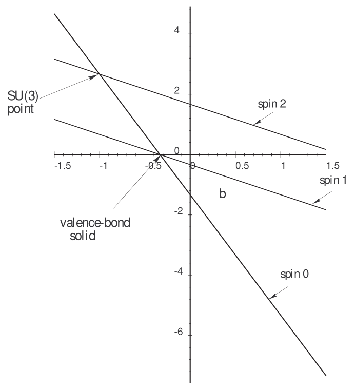
Figure 2: Energy levels for a two-site block for the Hamiltonian given by Eq. 69 for $-1\leq\beta\leq 1$.

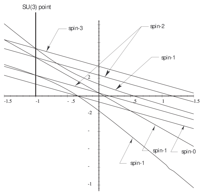
Figure 3: Energy levels for a three-site block for the Hamiltonian given by Eq. 69 for $-1\leq\beta\leq 1$.

The result of diagonalizing the two-site version of this Hamiltonian for $-1\leq\beta\leq 1$ is shown in Fig. 2 and the results for the three-site problem in Fig. 3, where I have limited discussion to the range $-1\leq\beta\leq 1$ for reasons which will become apparent. Note that due to the different numbers of eigenstates, etc., these plots look quite different from one another, however they share several important common features. First, observe that the lowest lying spin-$0$ and spin-$1$ state become degenerate at $\beta=-1/3$ and then cross one another. This level crossing means, as I said earlier, that any CORE computation which wishes to treat the region from $-1\leq\beta\leq 1$ must keep both multiplets; i.e., in either the two or three-site case, after the initial renormalization group step we arrive at a generalized Hamiltonian which forces us to adopt the two-site prescription of keeping the lowest lying spin-$0$ and spin-$1$ states. Second, it is worth noting that something very special happens at the point $\beta=-1$. In the two-site case we see that at this point the lowest lying multiplet is the three-dimensional spin-$1$ representation of $SU(2)$ and that the spin-$0$ and spin-$2$ states become degenerate and form a single six-dimensional subspace which in fact coincides with the six-dimensional representation of $SU(3)$. The degeneracy patterns shown here demonstrate that the Hamiltonian for $\beta=-1$ can be rewritten as

$$H_{\beta=-1}=\vec{Q}(i)\cdot\vec{Q}(i+1)$$ (70)

where the $\vec{Q}_{i}$’s stand for the generators of $SU(3)$. In this picture we see that the spin-$1$ representation can be identified as the triplet representation of $SU(3)$ and the degenerate multiplets of the two-site problem can be understood to be the $\overline{3}$ and $6$ representations of $SU(3)$ obtained from the tensor product of two $3$’s. A brief look at Fig. 3 supports this picture. Here we see that at $\beta=-1$ the $27$ states become one one-dimensional multiplet, two eight-dimensional multiplets and one ten-dimensional multiplet of degenerate states. This is, of course, completely consistent with what would be obtained from the product of three fundamental triplet representations of $SU(3)$ with the Hamiltonian given in Eq. 70. This explains my earlier statement that something interesting happens for $\beta=-1$ and shows that if one really wished to properly handle this point, it would be necessary to either adopt a truncation procedure which keeps more states, or one which goes beyond the range-2 cluster contribution in order to make up for the violence one is doing to the $SU(3)$ symmetry of the problem. Clearly, treating the full $SU(3)$ symmetry of the problem correctly would require us to eschew a two-site blocking procedure, since in this case the only non-trivial truncation would be to a single state. If we adopted a three-site blocking procedure then we could adopt a non-trivial truncation based upon keeping nine states, i.e., the lowest lying singlet and octet representations. Discussion of this problem goes beyond the scope of this paper. However I mention it to explain why one expects from the outset to have trouble using the four-state truncation algorithm which I will discuss for values of $\beta\leq-1$.

4.2 Spin-1 HAF: The Calculation

Since I just finished arguing that generically, after a single renormalization group step, one will have to deal with a Hamiltonian of the form

$$H=\sum_{i}\vec{s}(i)\cdot\vec{s}(i+1)-\beta\,(\vec{s}(i)\cdot\vec{s}(i+1))^{2}$$ (71)

I will describe the two-block CORE procedure for this generalized spin-$1$ HAF. As I already indicated, since this Hamiltonian doesn’t have a single-site term, the first step of the CORE computation is to solve the two-site problem exactly and truncate to the lowest spin-$0$ and spin-$1$ multiplets of the resulting nine state system (i.e., throw away the spin-$2$ multiplet). With this choice of projection operator the renormalized range-1 Hamiltonian is a diagonal $4\times 4$ matrix of the general form

$$h^{\rm conn}(j,1)=H_{\rm diag}=\left(\begin{array}[]{c c c c}\epsilon_{0}(\beta)&0&0&0\\ 0&\epsilon_{1}(\beta)&0&0\\ 0&0&\epsilon_{1}(\beta)&0\\ 0&0&0&\epsilon_{1}(\beta)\end{array}\right)$$ (72)

To obtain the range-2 term of the renormalized Hamiltonian we have to solve the two-block or four-site Hamiltonian exactly and use the information about the exact eigenvalues and eigenstates to construct $R$ and $H_{\rm diag}$. While in principle $R$ is a $16\times 16$ matrix, in practice, as in the case of the spin-$1/2$ HAF, the $SU(2)$ symmetry of the problem greatly simplifies the job of finding $R$ even though there aren’t enough symmetries to render the problem trivial. More precisely, the single-block states fall into a spin-$0$ and spin-$1$ representation of $SU(2)$ so, taking tensor products, we see that the retained states for the two-block problem are two spin-$0$ representations, three spin-$1$ representations and one spin-$2$ representation of this group. Clearly, if we expand any one of the spin-$2$ states in eigenstates of the four-site problem only states with the same quantum numbers can appear. Hence, since each of the spin-$2$ states is distinguished by its third component of spin, each of the spin-$2$ states will contract onto a different eigenstate of the two-block or four-site problem but they will all have the same energy. This argument shows that the transformation $R_{1}$ which takes us from the original tensor product basis to the spin basis is all one has to do for the spin-$2$ states. Since there are two independent spin-$0$ representations contained in the tensor product of the single-block states we have to do a bit more work to fully construct $R$. To understand exactly what has to be done, let $|{\Psi_{1}}\rangle$ and $|{\Psi_{2}}\rangle$ denote the spin-$0$ states which can be formed from the $0\otimes 0$ and $1\otimes 1$ representations of $SU(2)$. These states can be expanded in terms of spin-$0$ eigenstates of the two-block problem as

$$|{\Psi_{0}}\rangle = a_{0}|{\phi_{0}}\rangle+a_{1}|{\phi_{1}}\rangle+a_{2}|{\phi_{2}}\rangle+\ldots$$

$$|{\Psi_{1}}\rangle = b_{0}|{\phi_{0}}\rangle+b_{1}|{\phi_{1}}\rangle+b_{2}|{\phi_{2}}\rangle+\ldots$$

If, as will generally be the case, both $a_{0}$ and $b_{0}$ are non-vanishing, then both states will contract onto $|{\phi_{0}}\rangle$. One can always avoid this however by defining rotated states as follows

$$|{\chi_{0}}\rangle = \phantom{-}\cos(\theta)\,|{\Psi_{0}}\rangle+\sin(\theta)\,|{\Psi_{1}}\rangle$$

$$|{\chi_{1}}\rangle = -\sin(\theta)\,|{\Psi_{0}}\rangle+\cos(\theta)\,|{\Psi_{1}}\rangle$$ (74)

where $\cos(\theta)=a_{0}/\sqrt{a_{0}^{2}+b_{0}^{2}}$ and $\sin(\theta)=b_{0}/\sqrt{a_{0}^{2}+b_{0}^{2}}$. With this orthogonal change of basis we have

$$|{\chi_{0}}\rangle = \alpha_{0}|{\phi_{0}}\rangle+\alpha_{1}|{\phi_{1}}\rangle+\alpha_{2}|{\phi_{2}}\rangle+\alpha_{3}|{\phi_{3}}\rangle+\ldots$$

$$|{\chi_{1}}\rangle = \phantom{\alpha_{0}|{\phi_{0}}\rangle+\ }\beta_{1}|{\phi_{1}}\rangle+\beta_{2}|{\phi_{2}}\rangle+\beta_{3}|{\phi_{3}}\rangle+\ldots$$

With this definition $|{\phi_{0}}\rangle$ is the lowest lying eigenstate of the two-block Hamiltonian which appears in the expansion of $|{\chi_{0}}\rangle$ and $|{\phi_{1}}\rangle$ is the lowest lying eigenstate which appears in the expansion of $|{\chi_{1}}\rangle$; hence, if one applies $e^{-tH}$ to the rotated states one sees that $|{\chi_{0}}\rangle$ contracts onto $|{\phi_{0}}\rangle$ and $|{\chi_{1}}\rangle$ contracts onto $|{\phi_{1}}\rangle$.

The situation is exactly the same for the spin-$1$ states since the spin-$1$ state made out of $1\otimes 0-0\otimes 1$ is even under a reflection about the middle of the two-site block, whereas the spin-$1$ states made out of $1\otimes 0+0\otimes 1$ and $1\otimes 1$ are odd under the same reflection. This means that the expansion of the even spin-$1$ state cannot contain any eigenstates of the four-site problem in common with the expansion of the two odd spin-$1$ states. Thus, only the two odd spin-$1$ states need to be rotated into one another in order to guarantee that the lowest lying eigenstate appearing in the expansion of each state is unique, just as in the spin-$0$ case.

With this behind us, in the rotated basis, $H_{\rm diag}$ is a matrix whose diagonal entries are the eigenvalues of the lowest-lying eigenstates which appear in the expansion of the corresponding rotated state. Thus,

$$H_{2-block}(j,j+1) = RH_{\rm diag}R^{{\dagger}}$$

$$h^{\rm conn}(j,2) = H_{2-block}(j,j+1)-h^{\rm conn}(j,1)-h^{\rm conn}(j+1,1)$$ (76)

Finally, given these results we have the renormalized Hamiltonian defined on the thinner lattice

$$H^{\rm ren}=\sum_{j}\left(h^{\rm conn}(j,1)+h^{\rm conn}(j,2)\right)$$ (77)

As with all renormalization group algorithms, one iterates this process until the sequence of renormalized Hamiltonians either runs to a fixed point, or until one arrives at a situation which can be handled by perturbation theory. The generic step of the recursion follows the pattern just described, except that now the two-site Hamiltonian is defined to be

$$H_{2-site}(j,j+1)=h^{\rm conn}(j,1)+h^{\rm conn}(j+1,1)+h^{\rm conn}(j,2)$$ (78)

instead of Eq. 71. As before one diagonalizes $H_{2-site}(j,j+1)$ and retains the four lowest lying eigenstates which, if one starts out with $-1<\beta<1$, will be a spin-$0$ and spin-$1$ representation of $SU(2)$. From these states one constructs the new diagonal $h^{\rm conn}(j)$. Next, one constructs the new range-2 interaction by using these four states to construct the sixteen retained states for the two-block problem and expands them in terms of a complete set of eigenstates for the two-block Hamiltonian. From these expansions one determines $R$ and $H_{\rm diag}$, from which one immediately constructs the new $h^{\rm conn}(j,2)$. The results of running such iterations for starting values of $\beta=-1/3$ and $\beta=2/3$ are shown in Table 4 and Table 5 respectively.

The point $\beta=-1/3$ is one of the special points for which the theory based upon the Hamiltonian, Eq. 69 is exactly solvable, so it is interesting to see how the sequence of renormalization group transformations works for this case. Table 4 shows the results of the first and tenth iterations for the case $\beta=-1/2$. What is tabulated for each iteration are the eigenvalues and total spins, $S^{2}=S(S+1)$, for the eigenstates of the renormalized two-site Hamiltonian. As we see, initially the sixteen states of the two-site problem fall into irreducible representations of $SU(2)$ and while the states of each representation have the same energy, the different representations start out having distinct energies. This changes with increasing iterations until, as we see in the column for iteration ten, the system acquires a degenerate spin-$0$ and spin-$1$ multiplet and the remaining twelve states are all degenerate. This pattern reproduces itself unchanged for all succeeding iterations.

To understand what is happening in a simple way it is useful to rewrite this theory as a theory of spin-$1/2$ states. This can be easily done since each site of the lattice has both a spin-$0$ and spin-$1$ representation living on it and the product of two spin-$1/2$ representations contains exactly one spin-$0$ and one spin-$1$ representation, If we identify these representations with the four states per site of the original theory then we see that the Hilbert states of the original theory can be set in one-to-one correspondence with the states of a spin-$1/2$ theory on a lattice with twice as many sites. If we identify each two-site block, $B(2j,2j+1)$, with a single point of the original $\beta=-1/3$ theory, then the range-two reflection invariant Hamiltonian of the original theory must be equivalent to a generic range-four Hamiltonian of the form

$$H = \sum_{j}\left[\alpha{\bf 1}+A\vec{s}(2j)\cdot\vec{s}(2j+1)+B\vec{s}(2j+1)\cdot\vec{s}(2(j+1))\right.$$

$$+ C\vec{s}(2j)\cdot\vec{s}(2(j+1)+1)+D\vec{s}(2j)\cdot\vec{s}(2(j+1))$$ (79)

$$+ \left.D\vec{s}(2j+1)\cdot\vec{s}(2(j+1)+1))\right]$$

Now, since for the case $\beta=-1/3$ the spin-$0$ and spin-$1$ states are degenerate it follows that $A=0$, but at the starting level $B$, $C$ and $D$ do not vanish. Clearly one could obtain the exact values of these coefficients from the values of the level splittings in the first column of Table 4. The more interesting question is what values do these coefficients flow to as the number of iterations increase. Although one could do a brute force calculation of these results it is clear from the eigenvalues appearing in column two of Table 4 that the answer is that in this limit $A=C=D=0$ and $B=.8359471\ldots$ and $\alpha=3B/4$. With this choice of parameters we see that of the four spin-$1/2$ sites corresponding to the two-site block of the original theory, only the inner two spins are coupled to one another: i.e., the Hamiltonian for the block is just

$$H=3B/4{\bf 1}+B\vec{s}(2j+1)\cdot\vec{s}(2(j+1))=B/4+B(S^{\rm tot}(2j+1,2(j+1))/2-3/4)$$ (80)

From this we see that if the two inner spins are coupled to a spin-$0$ state then the two outer spins can be in any configuration (in particular either spin-$0$ or spin-$1$) producing four states of zero energy, which is what is seen. Furthermore, if the two inner spins are coupled to spin-$1$ then one gets $4\times 3=12$ degenerate states with energy $B$, which is also what is seen. Turning to the full renormalized Hamiltonian on the infinite lattice we see that the Hamiltonian describes a fully dimerized spin-$1/2$ system in which there is no coupling between two spins in the same block and the block-block couplings only exist between adjacent spins. It follows that the ground state of the infinite volume theory is one in which each pair of neighboring spins is coupled to spin-$0$. Note that this is reminiscent of the exact solution of this model as a valence bond solid [9]. The lowest lying excited states are those for which any one pair of interacting spins couples to a spin-$1$ state and all the others couple to a spin-$0$ state. If one is not at the renormalization group fixed point where $A=C=D=0$, but a small distance away, where these couplings are small but non-vanishing, then these degenerate states split into momentum bands. The interpretation of the fixed point gap is just the gap to all of the states which have arbitrarily small momentum in the infinite volume theory.

If we consider Table 5 we see quite a different picture, in that now the various multiplets are non-degenerate in the first iteration. Nevertheless, we see that after ten iterations the energy eigenvalues (to the accuracy shown) reproduce the same fixed point pattern as seen in the case $\beta=-1/3$ up to an overall constant. The only important difference between the case $\beta=-1/3$ and $\beta=2/3$ is that the gap for $\beta=2/3$ is smaller. Fig. 4 shows the result of carrying out renormalization group transformations for $-1<\beta<1.8$. Thus, the general picture emerging from this computation is that the spin-$1$ HAF in the region between $-1<\beta<1$ is controlled by the valence bond solid fixed point at $\beta=-1/3$ as one moves away from this point the mass goes down and at some point both above and below $\beta=1/3$ the theory appears to become massless. Given the limitation of the CORE computation to range two terms in the renormalized Hamiltonian it is not surprising the location of the points where the theory actually becomes massless is not very accurate. The dashed curve in Fig. 4 is not meant to be taken seriously, it is drawn in to guide the eye and remind the reader that the points $\beta=\pm 1$ are known to be massless theories; one expects that a computation going out to terms of range three or four would come closer to this picture. In any event, it seems clear from the picture that the point $\beta=0$, which is the spin-$1$ HAF, lies close enough to the $\beta=-1/3$ theory that one can be confident that it corresponds to a massive theory as conjectured. This of course is what we set out to show.

A final point worth commenting upon is the fact that no CORE computations were done for $\beta\leq-1$. The reason for this is that the truncation scheme used was to keep only the lowest lying spin-$0$ and spin-$1$ states. One trouble with this is that the program I used to compute the CORE transformation simply selected the four lowest lying states, which for the nondegenerate system in which the spin-$1$ and spin-$2$ have different energies worked fine. Unfortunately, this scheme breaks down at $\beta$ too near $-1$ and one ends up selecting four states but not necessarily all from either the spin-$0$ or the spin-$1$ multiplet. In this case one gets spurious results. To do the full job correctly would have required a more carefully written program. Another problem which contributes to the lack of accuracy of the range-2 calculation in the vicinity of $\beta=-1$ is that the theory develops an $SU(3)$ symmetry at $\beta=-1$ and so a truncation scheme which keeps only the spin-$0$ and spin-$1$ multiplets isn’t capable of manifestly preserving this symmetry. A scheme which did preserve the symmetry would need to keep full $SU(3)$ multiplets; i.e., the $SU(3)$ singlet state, which corresponds to the spin-$0$ state, and the full $SU(3)$ octet state, which corresponds to the sum of the spin-$1$ and spin-$2$ states. Note that while CORE allows one to choose a truncation scheme which doesn’t manifestly preserve the symmetries of the original theory and still obtain correct results, it does this at the expense of needing longer range couplings in the renormalized Hamiltonian in order to obtain high accuracy.

4.3 General $S$

In the preceding section I discussed the application of CORE to the spin-$1/2$ and spin-$1$ HAF, where simple range-2 arguments sufficed to show that, in agreement with the Haldane conjecture, the spin-$1/2$ HAF is a massless theory and that the spin-$1$ HAF is massive. What I did not discuss is what this analysis has to say about the case of the spin-$S$ HAF when $S$ is greater than one. A full analysis of the generic case requires doing a range-2 computation for all values of $S>1$, which I have not done. Nevertheless, examination of the key difference between these two computations suggests the physics which controls the general case.

To begin the discussion of the HAF for generic $S$ consider the first CORE transformation for an arbitrary $S$ HAF when one uses a three-site blocking procedure. (The reason for using a three-site algorithm is that there is no two-site blocking procedure which works for the spin-$1/2$ HAF.) For generic $S$ the three-site HAF Hamiltonian is given by Eq. 33 and the exact solution is as before, only the values for $S_{\rm TOT}(1,2,3)^{2}$ and $S_{\rm TOT}(1,3)^{2}$ change from case to case. It follows immediately that the lowest lying representation for the three-site problem is always spin $S$ and so, the state structure of the renormalized theory is the same as in the original theory, but as for the spin-$1$ HAF, the Hamiltonian changes. As always, truncating to the lowest lying representation yields a range-1 renormalized Hamiltonian which is simply a multiple of the unit matrix and so, the only real dynamics comes from computing the range-2 terms. In general, since the single-site retained states form a spin-$S$ representation, the two-site retained states decompose into a sum of representations going from $S^{{}^{\prime}}=0\ldots 2S$. Therefore, the new Hamiltonian can be written as a sum of terms

$$H=\sum_{j}\sum_{S^{{}^{\prime}}=0}^{2S}\epsilon_{S^{{}^{\prime}}}P_{S^{{}^{\prime}}}(j,j+1)$$ (81)

where $P_{S^{{}^{\prime}}}(j,j+1)$ is the operator which projects the tensor product states onto the spin-$S^{{}^{\prime}}$ representation and $\epsilon_{S^{{}^{\prime}}}$ is the eigenvalue of the lowest lying spin-$S^{{}^{\prime}}$ state appearing in the expansion of the projected tensor product state in terms of eigenstates of the two-block problem. Again, following the previous discussion, this Hamiltonian can always be rewritten as a polynomial in the operators $\vec{s}(j)\cdot\vec{s}(j+1)$. The important thing to notice at this point is that for integer $S$ and $\epsilon_{S^{{}^{\prime}}}=0$ for $S^{{}^{\prime}}=0\ldots S$ and $\epsilon_{S^{{}^{\prime}}}>0$, then the Hamiltonian is a theory of the form constructed by Affleck, Kennedy, Lieb and Tasaki (AKLT)[10] in order to exhibit theories having a valence-bond solid ground state. Thus, in the integer spin case any three-site CORE transformation immediately maps the integer spin HAF into a theory which has a massive valence-bond solid theory nearby. While it would take doing a complete computation of the CORE flows for this theory in order to prove that the spin-$S$ HAF lies in the basin of attraction of this theory, it is exactly what happened in the spin-$1$ case and it is not unreasonable to conjecture that this is the case for general $S$. The situation is quite different for theories with half-integer $S$. In such cases any three-site renormalization group transformation will map the theory into a sum of half-integral spin representations of $SU(2)$ with Hamiltonians of the form given in Eq. 81 and it is a theorem that an AKLT Hamiltonian for half-integral $S$ can’t have a valence-bond solid ground state. Generically, this result will coincide with what is found in a CORE computation, since for a half-integer spin a three-site truncation will always require that one keeps at least one irreducible representation per site which will perforce have dimension two or greater and these CORE calculations will generally iterate in a manner similar to the spin-$1/2$ theory; i.e., they will predict a massless theory, which is consistent with the Haldane conjecture. Of course, all this is conjecture and a real CORE calculation is needed for some higher spin theories in order to see how things really work.

5 Remarks About Correlation Functions

At this juncture it is important to emphasize that unlike the naive real-space renormalization group approach one cannot simply calculate long-distance behavior of a correlation function in the original theory by calculating the same function in the renormalized theory. This is because these correlation functions change in the same manner as the Hamiltonian does and they map into more complicated sums of operators which must be evaluated by the analogous CORE formula. An example of this is the computation of the magnetization in the Ising model discussed in Ref. [4].

6 Conclusion

In the preceding sections of this paper I exhibited explicit, first principles, CORE computations for the spin-$1/2$ and spin-$1$ HAF which showed that CORE is capable of high accuracy even when one keeps only a few states per block and a few terms in the cluster expansion. Moreover, I showed that even a simple range-2 approximation to a full CORE computation agreed for the spin-$1/2$ and spin-$1$ HAF predicts results in agreement with the predictions of the Haldane conjecture. I also argued that these computations suggest an attractive picture of how things can be expected to work for general $S$. I believe this set of results shows: first, that the usual folklore, which asserts that all real-space renormalization group methods which keep only a few states per block will be inaccurate, is incorrect; second, that even the simplest CORE computations are more than capable of providing revealing qualitative features which appear subtle from other points of view. These results buttress the hope that CORE can fruitfully be applied to the study of the complicated spin theories which are obtained from free fermion theories and theories of fermions interacting with gauge-fields which were obtained in Ref. [3]. The last point I would like to make is that these arguments show that although CORE does eventually depend upon one’s ability to do numerical computations, it has a strong semi-analytic flavor and is inherently different from Monte Carlo computations. CORE computations allow one to focus on the short distance Hamiltonian physics and the computation of renormalization group flows allows one to directly extract a physical picture of what is going on.

Table 1: Spin-1/2 HAF: Exact Energy Density = $-\ln(2)+1/4$ = -0.4431472

Range (sites)	Energy Density CORE	Padé [N/M]	Energy Density
1 (2)	-0.3750000
2 (4)	-0.4330127
3 (6)	-0.4387759	[1/1]	-0.4428182
4 (8)	-0.4406777	[1/2]	-0.4431005
		[2/1]	-0.4431022
5 (10)	-0.44155130	[2/2]	-0.4431337
6 (12)	-0.44202771	[2/3]	-0.4431412
		[3/2]	-0.4431412

Table 2: Spin-1 HAF : Compare to 16-Site Lanczos -1.40293

Range (sites)	Energy Density CORE	Padé [N/M]	Energy Density
1 (2)	-1.0000000
2 (4)	-1.3228757
3 (6)	-1.3622618	[1/1]	-1.3908701
4 (8)	-1.3771811	[1/2]	-1.3986541
		[2/1]	-1.3986795

Table 3: CORE flow for range-$4$ spin-$1/2$ HAF

Iter	${\cal E}$	$\alpha_{1}$	$\alpha_{2}$	$\alpha_{3}$	$\beta_{1}$	$\beta_{2}$	$\beta_{3}$
0	$-0.000000$	$1.000000$	$0.000000$	$0.000000$	$0.000000$	$0.000000$	$0.000000$
1	$-0.378606$	$0.477486$	$0.033980$	$0.013715$	$0.024739$	$0.069423$	$0.050919$
2	$-0.436439$	$0.179218$	$0.173143$	$0.007996$	$0.016203$	$-0.040886$	$0.026206$
3	$-0.443547$	$0.057900$	$0.005940$	$0.003327$	$0.006554$	$-0.167517$	$0.010529$
4	$-0.444307$	$0.016636$	$0.001615$	$0.001103$	$0.002175$	$-0.005772$	$0.003595$
5	$-0.444380$	$0.004270$	$0.000351$	$0.000116$	$0.000632$	$-0.001756$	$0.001090$
6	$-0.444385$	$0.000955$	$0.000050$	$0.000076$	$0.000163$	$-0.000477$	$0.000297$
7	$-0.444386$	$0.000170$	$0.000003$	$0.000016$	$0.000036$	$-0.000114$	$0.000073$
8	$-0.444386$	$0.000014$	$-0.000007$	$0.000003$	$0.000006$	$-0.000022$	$0.000015$

Table 4: CORE flow for case $\beta=-1/3$

Iteration 1		Iteration 10
Levels	${\bf S}^{2}$	Levels	${\bf S}^{2}$
0	0	0	0
0	2	0	2
0	2	0	2
0	2	0	2
0.89791173	6	0.83159471	6
0.89791173	6	0.83159471	6
0.89791173	6	0.83159471	6
0.89791173	6	0.83159471	6
0.89791173	6	0.83159471	6
0.94191045	2	0.83159471	2
0.94191045	2	0.83159471	2
0.94191045	2	0.83159471	2
1.1835034	2	0.83159471	2
1.1835034	2	0.83159471	2
1.1835034	2	0.83159471	2
1.8944584	0	0.83159471	0

Table 5: CORE flow for case $\beta=2/3$

Iteration 1		Iteration 10
Levels	${\bf S}^{2}$	Levels	${\bf S}^{2}$
-0.75395437	0	-1.6479538	0
1.1561163	2	-1.6479538	2
1.1561163	2	-1.6479538	2
1.1561163	2	-1.6479538	2
2.7471518	6	-1.1820317	6
2.7471518	6	-1.1820317	6
2.7471518	6	-1.1820317	6
2.7471518	6	-1.1820317	6
2.7471518	6	-1.1820317	6
3.520943	2	-1.1820317	2
3.520943	2	-1.1820317	2
3.520943	2	-1.1820317	2
4.6626764	0	-1.1820317	0
5.6297153	2	-1.1820317	2
5.6297153	2	-1.1820317	2
5.6297153	2	-1.1820317	2

Figure 1: Range-$3$ CORE $\beta$-function for spin-$1/2$ HAF

Figure 4: CORE predicted mass gap for $-1\leq\beta\leq 1$.

References

- [1] Papers in the particle physics and condensed matter literature which discuss applications of what I call the naive real-space renormalization group approach to various problems are: S. D. Drell, M. Weinstein and S. Yankielowicz, Phys. Rev. D14, 487 (1976); Phys. Rev. D14, 1627 (1976); Phys. Rev. D16,1769 (1977); R. Jullien, J. N. Fiels and S. Doniach, Phys. Rev. B16, 4889 (1977); S. D. Drell, B. Svetitsky and M. Weinstein, Phys. Rev., D17, 523 (1978); S. D. Drell and M. Weinstein, Phys. Rev. D17, 3203 (1978); J. W. Bray and S. T. Chui, Phys. Rev. B19, 4876 (1979); C. Y. Pan and Xiyao Chen, Phys. Rev. B36, 8600 (1987); M. D. Kovarik, Phys. Rev. B41, 6889 (1990).
- [2] S. R. White and R. M. Noack, Phys. Rev. Lett. 68, 3487 (1992); Steven R. White, Phys. Rev. B14, 10345 (1993).
- [3] Quarks, Gluons and Antiferromagnets, Marvin Weinstein, SLAC-PUB–8267, September 23, 1999
- [4] C.J. Morningstar and M. Weinstein, Phys. Rev. D54, 4131 (1996) hep-lat/9603016. ; Colin J. Morningstar and Marvin Weinstein, Phys. Rev. Lett. 73, 1873 (1994).
- [5] Djalma Medeiros and G. G. Cabrera, Phys. Rev. B43, 3703 (1991).
- [6] Adriana Moreo, Phy. Rev. B35, 8562 (1987).
- [7] F. D. M. Haldane, Phys. Lett. 93A, 464 (1983); Phys. Rev. Lett. 50, 1153 (1983).
- [8] P. W. Anderson, Phys. Rev. 88, 694 (1952).
- [9] An introduction to valence bond solid states can be found in the book Interacting Electrons and Quantum Magnetism, Assa Auerbach (Springer-Verlag, 1994). Details of carrying out computations of correlations in valence bond solids in one dimension can be found in D. P. Arovas, A. Auerbach, and F. D. M. Haldane, Phys. Rev. Lett., 60, 531 (1988).
- [10] I. Affleck, T. Kennedy, E. H. Lieb, and H. Tasaki, Phys. Rev. Lett., 59, 799 (1987)