EPHOU-00-001

NBI-HE-00-09

TIT/HEP-437

Jan. 2000

Recursive sampling simulations of
3D gravity coupled to scalar fermions

J. Ambjørn

Niels Bohr Institute
Blegdamsvej 17, Copenhagen Ø, Denmark
ambjorn@nbi.dk

D.V. Boulatov
Institute for Theoretical and Experimental Physics (ITEP)
B.Cheremushkinskaya 25, Moscow, Russia
boulatov@heron.itep.ru

N. Kawamoto
Physics Department, Hokkaido University
Sapporo, Japan

kawamoto@particle.sci.hokudai.ac.jp

Y. Watabiki
Tokyo Institute of Technology
Meguro, Tokyo, Japan
watabiki@th.phys.titech.ac.jp

Abstract

We study numerically the phase structure of a model of 3D gravity interacting with scalar fermions. We measure the 3D counterpart of the “string” susceptibility exponent as a function of the inverse Newton coupling $\alpha$. We show that there are two phases separated by a critical point around $\alpha_{c}\simeq 2$. The numerical results support the hypothesis that the phase structures of 3D and 2D simplicial gravity are qualitatively similar, the inverse Newton coupling in 3D playing the role of the central charge of matter in 2D.

1 Introduction

The success of the so-called dynamical triangulations or matrix models as a theory of 2D quantum gravity and non-critical strings has brought about a hope, that analogous discrete approaches might be useful in higher dimensions as well. The most natural way to introduce discretized quantum gravity is to consider simplicial complexes instead of continuous manifolds. Then, a path integral over metrics can be simply defined as a sum over all complexes having some fixed properties. For example, it is natural to restrict their topology. In the present paper, we consider only the 3-dimensional case, where, by definition, a simplicial complex is a collection of tetrahedra glued along their faces in such a way that any two of them can have at most one triangle in common. In addition we will restrict the topology to be that of the three-sphere.

To introduce metric properties, one can assume that complexes represent piece-wise linear manifolds constructed by gluing together equilateral tetrahedra [2]. The volume is then proportional to the number of them. In the continuum limit, as this number grows, the edge length, $a$, simultaneously tends to zero: $a\to 0$. In three dimensions, there is a one-to-one correspondence between classes of piece-wise linear and smooth manifolds. In other words, any homeomorphism can equally well be approximated by either a piece-wise linear or a smooth map. This property makes the model self-consistent.

Within a piece-wise linear approximation, the curvature is singular: the space is flat everywhere except at the edges. Therefore, one should consider integrated quantities, e.g. the mean scalar curvature

$$\int\!d^{3}x\,\sqrt{g}R\ =\ a\Big{(}2\pi N_{1}-6N_{3}\arccos\frac{1}{3}\Big{)}$$ (1.1)

where $a$ is the lattice spacing and $N_{0},\ N_{1},\ N_{2},\ N_{3}$ are the numbers of vertices, edges, triangles and tetrahedra, respectively.

For manifolds in 3 dimensions, the Euler character vanishes $\chi=N_{0}-N_{1}+N_{2}-N_{3}=0$. Together with the other constraint $N_{2}=2N_{3}$, it means that only 2 of the $N_{i}$’s are independent, $N_{1}=N_{0}+N_{3}$, and a natural lattice action depends on 2 dimensionless parameters. Now, we are in a position to define the simplicial-gravity partition function [3, 4, 5, 6]:

$${\bf Z}(\alpha,\mu)\ =\ \sum_{\{C\}}e^{\alpha N_{0}-\mu N_{3}}\ =\ \sum_{N_{3}}Z_{N_{3}}(\alpha)e^{-\mu N_{3}}$$ (1.2)

where $\sum_{\{C\}}$ is a sum over some class of complexes (e.g. of a fixed topology, as mentioned above). $\alpha=1/G$ is the inverse Newton constant and $\mu$ is the cosmological constant.

It can be shown that if $N_{3}$ is fixed, $N_{0}$ is restricted from above by $N_{0}<\frac{1}{3}N_{3}+const$. Therefore, it is natural, keeping $\alpha$ fixed, to let $\mu$ approach its critical value, $\mu_{c}$, at which the sum over $N_{3}$ in Eq. (1.2) becomes divergent. In the vicinity of $\mu_{c}$ one could hope to find critical behavior corresponding to a continuum limit of the model. In general the value of $\mu_{c}$ will be a function, $\mu_{c}(\alpha)$, of the other parameter $\alpha$. While $\mu\to\mu_{c}(\alpha)$ in general will correspond to an infinite volume limit ($N_{3}\to\infty$), it might require a fine-tuning of $\alpha$ to find a limit which has interesting continuum physics. From this point of view the parameter $\alpha$ might play a role similar to the one played by the (inverse) temperature $\beta$ in the Ising model. While we can take the infinite volume limit of the Ising model for any $\beta$, it is only for one specific value of $\beta$ (corresponding to the critical temperature) that we can relate the Ising model to a continuum $c=1/2$ conformal field theory.

For the model to be physically consistent, the free energy per unit volume, $\frac{1}{N_{3}}\log Z_{N_{3}}(\alpha)$, has to be finite. It implies that the series over $N_{3}$ in Eq. (1.2) has to have a finite radius of convergence: $0<\mu_{c}<+\infty$. If this holds, statistical models defined on such an ensemble of fluctuating lattices possess reasonable thermodynamical behavior. Thus one can hope to describe matter coupled to quantum gravity. This program has been successfully carried out in two dimensions with help of the matrix model techniques [7, 8]. In the 3D case, analytic tools are sparse and numerical simulations have so far been the main source of information. In the case of pure 3D gravity in references [4, 5], and in the case of matter fields coupled to 3D gravity in references [9].

Many questions, which are simple in two dimensions, become complicated in three. For example, 2-manifolds are classified according to values of the Euler character, and therefore topology, homotopy and homology are actually equivalent descriptions. In three dimensions, sets of manifolds characterized according to these 3 criteria are essentially different. From this point of view it is natural to ask how large a class of complexes $\{C\}$ one can include in Eq. (1.2), in order that the model still has acceptable properties, like being well defined and having a finite free energy per unit volume. It has been argued [10] that it is sufficient to fix only the first homology group $H_{1}(C,Z)$ in order to have a finite value of $\mu_{c}$. It can be reformulated as the following statement: “The number of simplicial manifolds constructed of the given number of tetrahedra, $N_{3}$, and having a fixed homology type (viz., the first Betti number and the torsion coefficients) grows at most exponentially as a function of $N_{3}$”.

Let us further note that the existence of such an exponential bound will remain valid if one attribute positive weights which grow at most exponentially with $N_{3}$, to every complex. The other way around, if one manages to represent a sum over complexes as a weighted sum over another class of objects, the weights again exponentially bounded, then it is sufficient to prove that the number of objects in the new class is exponentially bounded. In the class of regular triangulations there is firm numerical evidence for an exponential bound [11]. Further, analytical arguments now exist, which strongly favor an exponential bound [12].

The simplest example of a weighted sum of complexes is given by the canonical partition function $Z_{N_{3}}(\alpha)$ introduced in Eq. (1.2). Another example of physical interest is the partition function in the presence of free matter fields. To introduce it let us consider the set of polyhedral complexes dual to simplicial ones. Their 1-skeletons are some 4-valent graphs, $G^{(4)}$, whose vertices correspond to tetrahedra, and links are dual to triangles. Such a graph can be defined by the adjacency matrix

$$G^{(4)}_{ij}=\left\{\begin{array}[]{ll}1&\mbox{if vertices $i$ and $j$ are connected by a link}\\ 0&\mbox{otherwise}\end{array}\right.$$ (1.3)

Of course the set of 4-valent graphs is not identical to the totality of simplicial complexes. Similarly, in two dimensions, the set of ordinary $\phi^{3}$ Feynmann diagrams is different from that of triangulations – one has to introduce the notion of fat graphs to establish the equivalence.

If one attaches a $n$-component vector $x^{\mu}_{i}\ (\mu=1,\ldots,n)$ to the $i$-th vertex, the corresponding gaussian integral can be performed explicitly for every given graph $G^{(4)}$:

$$Z_{\rm matter}(G^{(4)})\ =\ \int\prod_{i=1}^{N_{3}-1}\prod_{\mu=1}^{n}dx^{\mu}_{i}\exp\Big{[}-\frac{1}{2}\sum_{i,j=1}^{N_{3}-1}G^{(4)}_{ij}(x^{\nu}_{i}-x^{\nu}_{j})^{2}\Big{]}\ =\ \Big{(}\det\mbox{}^{\prime}L^{(4)}\Big{)}^{-\frac{n}{2}}\,,$$ (1.4)

where the discrete Laplacian is given by

$$L^{(4)}_{ij}\ =\ 4\delta_{ij}-G^{(4)}_{ij}\,.$$ (1.5)

There is the nice combinatorial representation of the determinant given by Kirchoff’s theorem [16]:

$$\det\mbox{}^{\prime}L\ =\ |T(G)|\,,$$ (1.6)

where $T(G)$ is the set of all possible spanning trees embedded into a graph $G$ or, equivalently, the number of connected trees which can be obtained from the graph by cutting its links. To remove the zero mode in Eq. (1.4), we fixed the field at the $N_{3}$’th vertex. Kirchoff’s theorem states that $\det\mbox{}^{\prime}L$ does not depend on the choice of the vertex. Therefore, $|T(G)|$ is the number of rooted trees.

The number of spanning trees of a $k$-valent graph $G^{(k)}_{n}$ with $n$ vertices can be estimated from above as [16]

$$|T(G^{(k)}_{n})|\ \leq\ \frac{1}{n}\Bigg{(}\frac{nk}{n-1}\Bigg{)}^{n-1}\,.$$ (1.7)

The case we are particularly interested in is the 2-component Grassmann field (or equivalently, $n=-2$ in eq. (1.4)), where we obtain the gravity+matter partition function in the form

$${\bf Z}^{(1)}(\alpha,\mu)\ =\ \sum_{\{C\}}\det\mbox{}^{\prime}L\;e^{\alpha N_{0}-\mu N_{3}}\ =\ \sum_{N_{3}}Z^{(1)}_{N_{3}}(\alpha)e^{-\mu N_{3}}\,.$$ (1.8)

The weights, $\det\mbox{}^{\prime}L$, are positive integers, hence,

$$Z_{N_{3}}(\alpha)\ <\ Z^{(1)}_{N_{3}}(\alpha)\,.$$ (1.9)

In two dimensions, this type of matter has the central charge $c=-2$ and the corresponding matrix model has been solved explicitly by purely combinatorial means [7]. We can repeat the same trick in 3 dimensions:

$${\bf Z}^{(1)}(\alpha,\mu)\ =\ \sum_{\{C\}}\det\mbox{}^{\prime}L\;e^{\alpha N_{0}-\mu N_{3}}\ =\ \sum_{\{C\}}\sum_{\{\widetilde{T}(C)\}}e^{\alpha N_{0}-\mu N_{3}}\ =\ \sum_{\{\widetilde{T}\}}\sum_{\{C(\widetilde{T})\}}e^{\alpha N_{0}-\mu N_{3}}.$$ (1.10)

Here we have a sum over complexes, $\sum_{\{C\}}$, weighted with the number of spanning trees in the dual 1-skeleton of each complex, $\sum_{\{\widetilde{T}(C)\}}$. We can obtain exactly the same class of configurations by taking the sum over all possible trees, $\sum_{\{\widetilde{T}\}}$, weighted with the number of complexes, $\sum_{\{C(\widetilde{T})\}}$, which can be reconstructed from a given tree $\widetilde{T}$ by “restoring” links which we imagine have been cut in order to produce the tree from the original graph.

In three dimensions, the trees appearing this way correspond to spherical simplicial balls obtained starting with a single tetrahedron and subsequently gluing other tetrahedra to the faces of the boundary. If we denote by $n_{0},\ n_{1}$ and $n_{2}$ the numbers of vertices, edges and triangles on the boundary of a ball, we find that

$$n_{0}=N_{3}+3\,,\hskip 24.0ptn_{2}=2(N_{3}+1)\,.$$ (1.11)

It is convenient to weight every complex with the number of spanning trees $T$. This is an exponential reweighting of the kind discussed above. It can be done by introducing another system of free matter fields attached to vertices of triangulations. Then, analogously to Eq. (1.10), we define the modified partition function

$${\bf Z}^{(2)}(\alpha,\mu)\ =\ \sum_{\{C\}}\det\mbox{}^{\prime}L\;\det\mbox{}^{\prime}\widetilde{L}\;e^{\alpha N_{0}-\mu N_{3}}\,.$$ (1.12)

This partition function was used in [10] to prove that the number of simplicial 3-manifolds having a fixed homology type grows exponentially with the number of tetrahedra, as mentioned above. A priori it is not clear if ${\bf Z}^{(2)}(\alpha,\mu)$ defines a theory in the same universality class as the one defined by ${\bf Z}^{(1)}(\alpha,\mu)$. However, ${\bf Z}^{(2)}(\alpha,\mu)$ is the partition function of a set of Gaussian fields coupled to geometry in a well-defined way, and it is from this point of view equally interesting as the system defined by ${\bf Z}^{(1)}(\alpha,\mu)$. In the next section we consider a reduced version of (1.12).

2 Reduced model and connection with the 2-dimensional loop gas model

In 3 dimensions there are several natural choices of classes of complexes one can use in the definition of the partition function, as already discussed, and the question of universality classes is open. A simple choice is the set of 3-spheres with imbedded so-called 2-collapsible spines. A spine is the 2-skeleton, $K_{2}$, of a complex $C$ in a cell-decomposition with one 3-cell. In the simplicial context this 3-cell is a ball $B_{3}$ with a triangulated boundary. Thus we are lead to study the following partition function:

$${\bf Z}^{(2)}_{\rm red}(\alpha,\mu)\ =\ \sum_{C\sim S^{3}}\sum_{K_{2}\subset C}e^{\alpha N_{0}-\mu N_{3}}\sum_{T\subset K_{2}}\,,$$ (2.1)

where $\sum_{C\sim S^{3}}$ is the sum over all simplicial 3-spheres, where $\sum_{K_{2}\subset C}$ is the sum over 2-collapsible spines, $K_{2}$, embedded in $C$, and where $\sum_{T\subset K_{2}}$ is the sum over all spanning trees in $K_{2}$. The terms in (2.1) is a subset of the terms appearing in (1.12) when rewriting the determinant using a trick similar to the one used in (1.10) (see [10] for details). The spine $K_{2}$ in (2.1) is obtained from the 3-sphere $C$ a pair-wise identification (gluing) of all the boundary triangles. If $K_{2}$ is 2-collapsible, the pair-wise identification can be made “local” such that one can use recursively the gluing operation consisting of the identification of 2 triangles sharing a common link on the boundary, or, in other words, a folding along the link. In the dual language, one starts with an arbitrary spherical 3-valent fat graph and applies the move which can be represented as the flip of a link with the subsequent elimination of it:

(2.2)

Both of these moves are well known and have been used in Monte-Carlo simulations of triangulated surfaces [7]. Having glued all triangles, one finishes with a collection of self-avoiding closed loops, the number of which equals $N_{0}-1$.

It is convenient, instead of erasing a link after a flip, to decorate it with a dashed propagator and keep track of it in the process of subsequent foldings. To represent such configurations, we need to introduce the infinite set of vertices

(2.3)

which can be generated by successive flips. For example,
gives ;    gives ;   

or or give ;   

or or or give ,   

and so on.

In the end, we obtain planar diagrams with two types of propagators: solid ones produce closed loops while dashed form arbitrary clusters of dotted lines. The total number of vertices is equal to $2(N_{3}+1)$. We weight every loop with the numerical factor $e^{\alpha}$.

Thus, the model can be represented as a non-local gas of closed loops with the partition function

$${\bf Z}^{(2)}_{\rm red}(\alpha,\mu)\ =\ \sum_{\{{\cal D}\}}w_{\cal D}\,e^{\alpha N_{0}-\mu N_{3}}\,,$$ (2.4)

where $\sum_{\{{\cal D}\}}$ is the sum over all the diagrams. The weight $w_{\cal D}$ is equal to the number of inequivalent starting configurations giving the same planar diagram $\cal D$ (can be 0). The number of closed loops is simply equal to $N_{0}-1$ and $\alpha$ can be identified with the inverse Newton constant.

We see that the weights $w_{\cal D}$ in Eq. (2.4) in principle are recursively calculable. However, from a practical point of view it is difficult to take into account the entropy of the configurations, and the model (2.4) seems to be analyticlly unsolvable. Therefore, let us consider the localized version of the model, namely, the dense phase of the self-avoiding loop gas matrix model (in the following simply denoted the loop gas (LG) model):

$$Z_{\rm LG} = \int d^{\scriptscriptstyle N^{2}}Y\prod_{\nu=1}^{n}d^{\scriptscriptstyle N^{2}}X_{\nu}\exp\Big{[}-\frac{N}{2}{\rm tr}\;Y^{2}-\frac{N}{2}\sum_{\nu=1}^{n}{\rm tr}\;X^{2}_{\nu}+\frac{N}{2}\sum_{\nu=1}^{n}{\rm tr}\;YX^{2}_{\nu}\Big{]}$$ (2.5)

$$= \int d^{\scriptscriptstyle N^{2}}Y\exp\Big{[}-\frac{N}{2}{\rm tr}\;Y^{2}-\frac{n}{2}{\rm tr}\;^{2}\log\Big{(}1\otimes 1-\mu Y\otimes 1-1\otimes\mu Y\Big{)}\Big{]}\,.$$

Here $Y$ and $X_{\nu}$ are hermitian $N\times N$ matrices. We have attached the lower index to the gaussian $X_{\nu}$ variable to weight every closed loop with the factor $n\equiv e^{\alpha}$. In the $N\to\infty$ limit, this model generates planar diagram having only the simplest 3-valent vertices from the whole series (2.3). For such diagrams, all the weights in Eq. (2.4) are trivial: $w_{\cal D}=1$.

This truncated local model might have some qualitative features in common with 3-dimensional simplicial gravity. It seems to be a reasonable assumption, because the corresponding universality class is very large, (see Ref. [8]), and includes all local perturbations of the model (2.5). On the other hand, multiple overlapping sequences of the flips can be regarded as a kind of renormalization group procedure, which could draw any given system to a stable fixed point in the space of all planar-graph models. It looks a bit more natural in dual terms. One takes an arbitrary spherical ball with a huge triangulated boundary and uses subsequently and randomly the folding operation (dual to the flip). Soon the boundary triangulation will be randomized. If this randomization has appropriate robust statistical properties, we would expect to find many models falling in the same universality class.

Then any 2 models from the same universality class should be identical in their continuum limits.

The critical behavior of the loop gas matrix model is well known. For $n<2$, it describes 2D gravity interacting with $c<1$ conformal matter

$$c\ =\ 1-6\frac{(1-g_{0})^{2}}{g_{0}};\hskip 24.0ptn\ =\ -2\cos\pi g_{0}\,,$$ (2.6)

while for $n>2$ the corresponding matter is non-critical and the model trivializes except in special situations [13]. In this phase, the number of closed loops is proportional to the volume and the mean length of each remains finite.

In the vicinity of a critical point $\mu_{c}$, the partition function behaves as

$$Z_{\rm LG}\ \approx\ (\mu_{c}-\mu)^{2-\gamma_{\rm str}}\,.$$ (2.7)

This formula defines the famous string susceptibility exponent $\gamma_{\rm str}$.

Two main quantities of interest are

$$\langle N_{3}\rangle_{LG}\ =\ \frac{\partial\ }{\partial\mu}\log Z_{\rm LG}\ \approx\ -(2-\gamma_{\rm str})\frac{\mu_{c}}{\mu_{c}-\mu}$$ (2.8)

and

$$\langle N_{0}\rangle_{LG}\ =\ \frac{\partial\ }{\partial\alpha}\log Z_{\scriptscriptstyle LG} \approx (2-\gamma_{\rm str})\frac{\mu^{\prime}_{c}(n)}{\mu_{c}(n)-\mu}\,-\,\frac{\partial\gamma_{\rm str}}{\partial\alpha}\log|\mu_{c}-\mu|$$ (2.9)

$$\approx -\frac{\mu^{\prime}_{c}}{\mu_{c}}\langle N_{3}\rangle_{LG}\,+\,\frac{\partial\gamma_{\rm str}}{\partial\alpha}\log\langle N_{3}\rangle_{LG}$$

where the coefficients can be calculated explicitly using the Gaudin and Kostov’s exact solution [8]

$$\frac{\partial\ }{\partial n}\log\mu_{c}\ =\ -\frac{1}{2}\frac{1}{n+2};\hskip 24.0pt\frac{\partial\gamma_{\rm str}}{\partial n}\ =\ \frac{1}{2\pi g_{0}^{2}\sin\pi(1-g_{0})}\,.$$ (2.10)

If $2-n\ll 1$, then

$$\langle N_{0}\rangle_{LG}\ \approx\ \frac{1}{4}\langle N_{3}\rangle_{LG}\,+\,\frac{1}{\pi\sqrt{2-n}}\log\langle N_{3}\rangle_{LG}\,.$$ (2.11)

If $n>2$, then $\gamma_{\rm str}$ is independent of $n$ and $\langle N_{0}\rangle_{LG}$ is proportional to $\langle N_{3}\rangle_{LG}$, except in special situations [13].

3 Numerical experiments

Unfortunately, the nonlocal model (2.4) looks analytically unsolvable. However, it can be successfully simulated numerically by the recursive sampling-Monte-Carlo technique. It is natural to use a recursive sampling to perform the summation over the tree-dual balls in a close analogy with Ref. [17]. Then, a Metropolis algorithm can be used to produce a random walk in a space of all simplicial spherical balls. Closed manifolds appear when the boundary of a ball is shrunk, again by a trial and error Monte Carlo procedure. In the following we describe the algorithm in some detail.

3.1 The algorithm for generating three-spheres

As mentioned, a recursive algorithm has been used with great success for a $c=-2$ model coupled to two-dimensional quantum gravity. Since our model resembles the $c=-2$ model quite a lot, it is natural to try to use the same technique in three dimensions. One of the main reasons for the success of the algorithm in the two-dimensional case was that the branching probability of tree-graphs and the counting of rainbow diagrams could be calculated analytically. In the present three-dimensional model the branching probability can be calculated analytically, as shown below. However, while there is a three-dimensional analogy of the rainbow diagram encountered in two dimensions, they are not two-dimensional extended objects and we do not know how to count them.

Let us calculate the branching probability of 3-valent tree-diagrams. The Schwinger-Dyson equation for 3-valent graphs corresponding to Fig. 1 is

$$T\ =\ xT^{3}+1,$$ (3.1)

where $T(x)$ is the generating function for the number of tree diagrams, i.e.,

$$T(x)\ =\ \sum_{n}t_{n}x^{n},$$

where $t_{n}$ is the number of 3-valent tree-diagrams with $n$ vertices.

Figure 1: Graphical presentation of Schwinger-Dyson equation for 3-valent tree-diagrams.

Since the Schwinger-Dyson equation is a cubic equation with respect to $T$, it has three solutions. We have to select the unique solution which satisfies the physically imposed boundary condition $t_{0}=1$. This results in the following solution:

$$T\ =\ \frac{3}{z}\,\sinh\Bigl{(}\frac{1}{3}\log(z+\sqrt{1+z^{2}})\Bigr{)},~{}~{}~{}~{}z=i\sqrt{\frac{27x}{4}},$$ (3.2)

which has the following power series expansion:

$$T(x)\ =\ \sum_{n=0}^{\infty}t_{n}x^{n}\ =\ \sum_{n=0}^{\infty}\frac{(3n)!}{n!(2n+1)!}\,x^{n}.$$ (3.3)

We can now define the probability of the 3-valent tree-diagrams with $k$ vertices branching into tree-diagrams with $l$, $m$ and $n$ vertices

$$w(l,m,n)\ =\ \frac{t_{l}t_{m}t_{n}}{t_{k}}~{}~{}~{}~{}~{}~{}~{}(l+m+n=k-1),$$ (3.4)

which then naturally satisfies

$$\sum w(l,m,n)\ =\ 1,$$ (3.5)

where the summation is over $l,m,n\geq 0$ with the constraint $l+m+n=k-1$. By rearranging the summation we obtain the following relation

$$w(l,m,n)\ =\ w_{1}(l)\,w_{2}(m,n),$$ (3.6)

where

$$w_{1}(l)=\sum_{\mbox{\scriptsize{$\matrix{m^{\prime},n^{\prime}\geq 0\cr m^{\prime}+n^{\prime}=k-l-1}$}}}w(l,m^{\prime},n^{\prime}),~{}~{}~{}~{}w_{2}(m,n)=\frac{w(l,m,n)}{w_{1}(l)},$$ (3.7)

where $m+n=k-l-1$. Since we have the relations

$$\sum_{l=0}^{k-1}w_{1}(l)\ =\ 1,~{}~{}~{}~{}~{}\sum_{\mbox{\scriptsize{$\matrix{m,n\geq 0\cr m+n=k-l-1}$}}}w_{2}(m,n)\ =\ 1,$$ (3.8)

we can divide the branching process into two parts using the relation

$$\sum_{\mbox{\scriptsize{ $\matrix{m,n\geq 0\cr m+n=k-l-1}$}}}w(l,m,n)\ =\ \frac{3(k-l)-2}{k-l}\;\frac{t_{l}t_{k-l-1}}{t_{k}}~{}~{}~{}~{}~{}(0\leq l\leq k-1),$$ (3.9)

and write:

$$w_{1}(l)\ =\ \frac{3(k-l)-2}{k-l}\;\frac{t_{l}t_{k-l-1}}{t_{k}},~{}~{}~{}~{}w_{2}(m,n)\ =\ \frac{k-l}{3(k-l)-2}\;\frac{t_{m}t_{n}}{t_{m+n}}.$$ (3.10)

Using these analytic formulas we can set up a recursive sampling algorithm for constructing 3-valent tree-diagrams in three dimensions.

In order to construct a three-dimensional simplicial manifold with the topology of $S^{3}$ from the 3-valent diagrams, we need to identify the “end branches” of the tree-diagrams in the dual diagram sense, or equivalently, successive neighboring triangles of the corresponding original manifold. In contrast to the two-dimensional $c=-2$ model, where an analytic formula for the number of rainbow diagrams is given, it is presently unknown how to obtain a closed expression in the three-dimensional case since the trees are now genuine three-dimensional objects. The initial three-dimensional tree diagram corresponds to the tree shape volume object which has a ball topology with a triangulated $S^{2}$ sphere as a boundary. It should be noted that in this model all the links of the corresponding three-dimensional simplicial manifold are on the boundary in the initial tree configuration. We first randomly pick up a link on the boundary and identify the neighboring triangles which share the link as a common one. This link is now hidden inside from the boundary. We then pick up another link which is on the boundary surface and repeat the gluing procedure of the triangles. This procedure should be continued successively until all the triangles on the boundary surface are identified (and the boundary thereby has vanished). Since we don’t know the analytic expression of the weight factor of the three-dimensional “rainbow diagrams”, we need to introduce the ungluing process and use a Monte Carlo simulation to obtain a typically triangulated three-dimensional $S^{3}$ sphere in our model. Since the gluing process is carried out by a Monte Carlo algorithm, we operate both with the gluing process and its reciprocal in such a way that the usual detailed balance is fulfilled. In this procedure the order of gluing and ungluing processes, which are reflected in the internal configuration of the simplicial manifold, are important and thus should be memorized in the simulation. In this Monte Carlo procedure there is unavoidably introduced an iteration uncertainty in the counting procedure.

3.2 Observables

After constructing typical $S^{3}$ manifolds one can use these to calculate expectation values of observables. A basic observable which probes the phase diagram of the model is the “string” susceptibility exponent $\gamma$ defined analogously to Eq. (2.7). The most convenient way to extract $\gamma$ is by means of the so-called baby universe technique [18], which contrary to the original definition (2.7) allows us to extract $\gamma$ from an ensemble of manifolds with fixed volume $N_{3}$. One counts the configurations of three-manifolds which are separated into two parts via a common triangle, and then measures the volumes $M_{3}$ and $N_{3}-M_{3}$ of the separated parts. The string susceptibility is then derived from the following relation:

$$W(M_{3})\ =\ \frac{M_{3}Z(M_{3})\;(N_{3}-M_{3})Z(N_{3}-M_{3})}{Z(N_{3})}\ \sim\ N_{3}\left[\frac{M_{3}}{N_{3}}\Big{(}1-\frac{M_{3}}{N_{3}}\Big{)}\right]^{\gamma-2},$$ (3.11)

where the partition function $Z(N_{3})$ (in accordance with (2.7)) is assumed to be parametrized as $Z(N_{3})\sim N_{3}^{\gamma-3}\;e^{-\mu_{c}N_{3}}$. In particular we obtain the following approximate scaling function:

$$F(x)\ =\ N_{3}\log\frac{W(M_{3}+1)}{W(M_{3})}\ \sim\ (\gamma-2)\left(\frac{1}{x}-\frac{1}{1-x}\right),$$ (3.12)

where the scaling parameter is $x=M_{3}/N_{3}$.

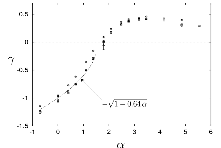
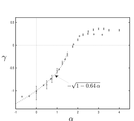
Figure 2: “String” susceptibility $\gamma$ versus $\alpha$, the inverse Newton constant, for $N_{3}=50$($\diamond$), $100$($-$), $200$($\Box$), $300$($\times$) above and $N_{3}=300$($\diamond$), $500$($-$) below.

A number of measured values of $\gamma$ as a function of $\alpha$, the inverse Newton constant, is shown in Fig. 2. Statistical error-bars are shown in the Figure. The two sub-figures in Fig. 2 represent independent measurements for the different value of $N_{3}$ and they agree perfectly within error-bars. Systematic errors (e.g. due to finite size effects) seem to be of the same order except in a vicinity of the transition point. The data are collections of three simulations which took place approximately 4-6 months of CPU time for each calculation on a Pentium 200 MHz personal computer and HP Convex and Origin 2000 parallel computers. We have collected data for $N_{3}=50$, $100$, $200$ at $\log(1/2)\leq\alpha\leq\log(256)$, and $N_{3}=300$ at $\alpha=0$ and have shown the extracted $\gamma$ in the upper sub-figure of Fig. 2. Other data for $N_{3}=300$, $500$ lead the $\gamma$-values shown in the lower sub-figure. Although the number of tetrahedra are small, they seem to give reliable measurements of $\gamma$ in the interval $-0.7<\alpha<5.5$, except for $N_{3}=50$. For the value of $N_{3}$ there is a systematic deviation from the other values, probably caused by the small number of $N_{3}$. A typical distribution of $\log W(M_{3})$ for $\alpha=0$ and $N_{3}=300$ is shown in Fig. 3 where the slope of the curve determines $\gamma$.

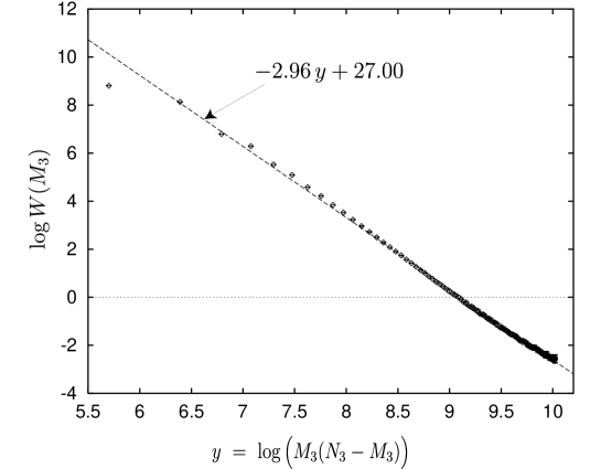
Figure 3: $\log W(M_{3})$ versus $\log\big{(}M_{3}(N_{3}-M_{3})\big{)}$ at $\alpha=0$ for $N_{3}=300$.

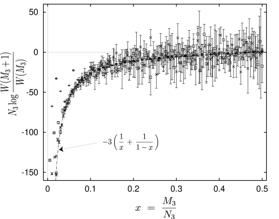
Figure 4: Scaling function $F(x)$ versus $x=M_{3}/N_{3}$ at $\alpha=0$ for $N_{3}=50$, $100$, $200$, $300$.

The scaling function $F(x)$ with the predicted curve (3.12) is shown in Fig. 4 for $\alpha=0$ with $N_{3}=50$, $100$, $200$, $300$. We can see that all the data scale nicely within the error-bars except for $M_{3}<\raisebox{-5.69054pt}{$\sim$}~{}M_{3}^{\rm min}=5$. As the formula (3.12) is valid only asymptotically, we can use fitting only for values of $M_{3}$ bigger than some cutoff $M_{3}^{\rm min}$. The independence of results from this cutoff can serve as an indicator of the reliability. A corresponding typical measurements are shown in Fig. 5. For small values of $M_{3}<\raisebox{-5.69054pt}{$\sim$}~{}M_{3}^{\rm min}=5$, the measured “virtual” values of $\gamma$ oscillate and for larger values they gradually converge to a stable limit.

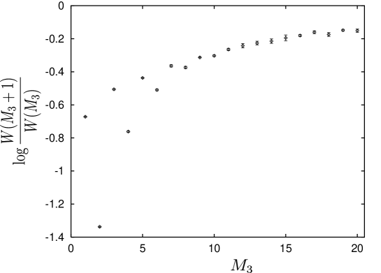
Figure 5: $\hbox{log}\frac{W(M_{3}+1)}{W(M_{3})}$ versus $M_{3}$ at $\alpha$ = 0 for $N_{3}$ =300.

In the measurements of $\gamma$ we have thus collected the data satisfying $M_{3}>\raisebox{-5.69054pt}{$\sim$}~{}M_{3}^{\rm min}+1=6$. We have measured $\gamma$ with good statistics for $\alpha=0$ where we collected $10^{5}$ configurations while for the other values we collected about $2\times 10^{4}$ configurations. The measured value $\gamma$ is so close to $-1$ that it is tempting to conjecture that this is the exact value for $\alpha=0$. One could hope that it was possible to prove this result analytically, since it corresponds to the strong coupling limit $G=1/\alpha=\infty$.

4 Discussion

The results of the numerical experiments give some support to the idea that there should be a qualitative similarity of the phase structures of 2- and 3-dimensional simplicial gravities with Newton’s coupling constant playing a role analogous to the matter central charge in 2 dimensions. A similar idea can be found in a slightly different context in [15]. The experimental values of $\gamma$ shown in Fig. 2 support the picture of 2 phases with the critical coupling $\alpha_{\rm c}\approx 2$. For $\alpha<\alpha_{\rm c}$, the simplest square root function

$$\gamma\ =\ -\sqrt{1-0.64\,\alpha\,}$$ (4.1)

fits surprisingly well the experimental points. We show the above expression by the dotted curve in Fig. 2. For $\alpha>\alpha_{\rm c}$, $\gamma$ is a constant within error bars about $0.3$. Since the systems are quite small, and since there still is some drift in the extracted values of $\gamma$ towards larger values when $N_{3}$ is increased (see in particular lower sub-figure in Fig. 2), we cannot conclude if $\gamma=1/2$ in the limit of infinite $N_{3}$ or if $\gamma=1/3$, which is the next lowest value that $\gamma$ can have in the branched polymer phase [14].

From a theoretical point of view, it has been recognized by H. Kawai and one of authors (Y.W.) that in the case of $D>2$ and around $1/\alpha=G=0$, the branched configurations give much more dominant contribution to the path-integral over metrics than the configurations near the flat space-time[19]. Let us consider the scaling property of

$$X\ =\ \exp\!\bigg{(}\frac{1}{G}\int\!\!\sqrt{g}R\bigg{)}\,.$$ (4.2)

Near flat space-time dimensional analysis is reliable and leads to $\int\!\!\sqrt{g}R\sim V^{1-\frac{2}{D}}$. Then one finds

$$X\ \sim\ \exp\!\bigg{(}\hbox{const.}\frac{V^{1-\frac{2}{D}}}{G}\bigg{)}\,,$$ (4.3)

where $V$ is the volume of space-time. On the other hand, for branched polymer like configurations it is easy to show that i.e. $\int\!\!\sqrt{g}R\sim V$. Thus one finds in this case that

$$X\ \sim\ \exp\!\bigg{(}\hbox{const.}\frac{V}{G}\bigg{)}$$ (4.4)

instead of (4.3). Comparing eqs. (4.3) and (4.4) around $G\sim 0$, one finds that (4.4) gives a more dominant contribution to the path-integral than the contribution (4.3) from flat space. This is one reason why one cannot perform the quantization of gravity perturbatively around the flat space-time (except for the very special cases when $1/\alpha_{\rm c}=G_{\rm c}=0$). This theoretical observation is consistent with the result of this paper.

If we accept the result that there are two phases in the present model of 3-dimensional simplicial gravity, then the next natural question to ask is: “How large is the corresponding universality class?” Does the complete model (1.12) with a sum over all 3-spheres belong to the same class? It seems plausible, but it is difficult to judge how restricted the subset of simply connected 3-manifolds taken into account in the simulated statistical ensemble really is. It is not easy to construct a simplicial 3-sphere which would not be included in it. At first thought, Zeeman’s Dunce Hat[20] could serve as a mean to construct a counter example. Triangles belonging to a boundary of an initial ball cannot form such a pseudosurface after local foldings. However, those lying inside the ball can. Even in the simplest case of 2 tetrahedra, a Zeeman’s Dunce Hat can easily be obtained. Further, the construction given in Ref. [21] is not a “counter example” because it is not a triangulation. On the other hand, there is an old result of Haken [22] who showed that any 3-sphere possesses an obviously trivial presentation of $\pi_{1}$ (in the sense that it can be trivialized by a sequence of simple substitutions of the length less or equal than 4). Unfortunately, this result does not imply that any simplicial 3-sphere allows for at least one 2-collapsible spine (if it did, the famous Poincaré hypothesis would be simultaneously proven). It seems an open question whether any simplicial 3-sphere is counted at least once in the partition function (2.4). If it is the case, then only the matter sector of the original model (1.12) is distorted by our simplifications leading to the reduced model. Even if not all 3-spheres are included in the model, it seems reasonable to conjecture that the reduced model and the original model belong to the same universality class as far as their continuum limits are concerned.

Acknowledgements

J.A. acknowledges the support of MaPhySto, Centre of Mathematical Physics and Stochastics, which is financed by the Danish National Research Foundation. This work is supported in part by Japanese Ministry of Education under the Grant-in-Aid number 09640330 and the special funding for basic research under the project name “Hierarchical Structure of Matter Analyzing system”.

References

- [1]
- [2] T. Regge, Nuovo Cimento 19 (1961) 558.
- [3] J.Ambjørn, B.Durhuus and T.Jonsson, Mod. Phys.Lett. A6 (1991) 1133.
-
[4]
M.E. Agishtein and A.A. Migdal, Mod. Phys. Lett.
A6 (1991) 1863;
J.Ambjørn and S. Varsted, Phys. Lett. B226 (1991) 258 and Nucl. Phys. B373 (1992) 557. -
[5]
D.V. Boulatov and A. Krzywicki, Mod. Phys. Lett. A6
(1991) 3005;
J.Ambjørn, D.V. Boulatov, A. Krzywicki and S. Varsted, Phys. Lett. B276 (1992) 432. - [6] D.V.Boulatov, Mod. Phys. Lett. A7 (1992) 1629 and “3D gravity and gauge theories”, hep-th/9311088.
- [7] V.A.Kazakov, I.K.Kostov and A.A.Migdal, Phys.Lett. B157 (1985) 295; D.V.Boulatov, V.A.Kazakov, I.K.Kostov and A.A.Migdal Nucl. Phys. B275 (1986) 641.
- [8] I.K.Kostov, Mod. Phys. Lett. A4 (1989) 217; M.Gaudin and I.K.Kostov, Phys. Lett. B220 (1989) 200.
- [9] J. Ambjørn, Z. Burda, J. Jurkiewicz, and C.F. Kristjansen, Phys. Lett. B297 (1992) 253.
- [10] D.V.Boulatov “On entropy of 3-dimensional simplicial complexes”, hep-th/9408012; JHEP 07(1998)010, hep-th/9804078.
-
[11]
J.Ambjørn and S. Varsted, Phys. Lett. B226 (() 1991) 258 and Nucl. Phys. B373 (1992) 557.
S. Catterall, J. Kogut and R. Renken: Phys.Lett. B342 (1995) 53-57. -
[12]
M. Carfora and A. Marzuoli:
Entropy estimates for simplicial quantum gravity,
J. Geom. Phys. 16 (1995) 99-119;
Holonomy and entropy estimates for dynamically triangulated manifolds, J. Math. Phys. 36 (1995) 6353-6376.
J. Ambjørn, M. Carfora and A. Marzuoli: The geometry of dynamical triangulations, Lecture Notes in Physics, New Series, m50, Springer, Berlin, 1997, hep-th/9612069. -
[13]
B. Durhuus and C. Kristjansen,
Nucl.Phys. B483 (1997) 535-551.
B. Eynard and C. Kristjansen, Nucl.Phys. B466 1996) 463-487. -
[14]
J. Ambjorn, B. Durhuus and T. Jonsson,
Mod.Phys.Lett. A9 (1994) 1221-1228.
J. Ambjorn, Gudmar Thorleifsson and Mark Wexler, Nucl.Phys. B439 (1995) 187-204. -
[15]
I. Antoniadis and Emil Mottola,
Phys.Rev. D45 (1992) 2013-2025.
I. Antoniadis, Pawel O. Mazur and Emil Mottola, Nucl.Phys. B388 (1992) 627-647; Phys.Lett. B323 1994) 284-291. - [16] N.Biggs, Algebraic graph theory, Cambridge (1974).
- [17] N.Kawamoto, V.A.Kazakov, Y.Saeki and Y.Watabiki, Phys. Rev. Lett. 68 (1992) 2113.
- [18] J.Ambjørn, S.Jain, J.Jurkiewicz and C.F.Kristiansen, Phys. Lett. B305 (1993) 208.
- [19] H.Kawai and Y.Watabiki, unpublished.
- [20] E.C.Zeeman, Topology 2 (1964) 341.
- [21] B.Durhuus and T.Jonsson, Remarks on the entropy of 3-manifolds, hep-th/9410110.
- [22] W.Haken, Illinois J. Math. 12 (1968) 133.