The 1 Teraflops QCDSP computer

Abstract

The QCDSP computer (Quantum Chromodynamics on Digital Signal Processors) is an inexpensive, massively parallel computer intended primarily for simulations in lattice gauge theory. Currently, two large QCDSP machines are in full-time use: an 8,192 processor, 0.4 Teraflops machine at Columbia University and an 12,288 processor, 0.6 Teraflops machine at the RIKEN-BNL Research Center at Brookhaven National Laboratory. We describe the design process, architecture, software and current physics projects of these computers.

1 Introduction

The search for the smallest constituents of matter has led to the discovery of many sub-atomic particles and the development of the standard model of particle physics. This model is based on the principle of “local gauge invariance”, first seen in Maxwell’s theory of electromagnetism, where it constrains the types of interactions possible between photons and electrons. The standard model includes the strong, weak and electromagnetic forces, providing a description of virtually all experimental phenomenon seen to date. It is a theory of generalized force-carrying particles of spin one interacting with matter that is either fermionic (spin one-half) or bosonic (spin zero).

The principle of local gauge invariance is an important abstract idea, similar to the concept of evolution in biology, but as embodied in the standard model it also leads to a quantitative theory which describes particle interactions precisely. Many comparisons between standard model predictions and experiment have been made, primarily involving the weak and electromagnetic part of the model or the strong force at high energies. At low energies (up to a few GeV) the strong force (described by a part of the standard model known as quantum chromodynamics, QCD) is not analytically tractable in any reliable approximation, making quantitative predictions in this region solely accessible by computational techniques. As a simple example, most of the proton’s properties are completely determined by QCD, but cannot be calculated from first principles.

The lack of precise predictions from QCD is currently a restriction on further tests of the standard model and our ability to understand new phenomena to be probed by experiment. QCD is formulated in terms of quarks (spin one-half particles) and gluons, which mediate the strong force. The electroweak interactions of quarks are given by the standard model, but many of the manifestations of these interactions are only visible in physical particles (hadrons) which are bound states of quarks. Precise predictions from QCD for electroweak processes requires knowing precise information about the quark content of hadrons. In addition, the RHIC (Relativistic Heavy Ion Collider) at Brookhaven National Laboratory will soon begin colliding nuclei at high energies to probe nuclear matter at high temperatures and densities. Once again analytic calculations here are limited, even though the underlying physical formulation is presumed understood.

2 Lattice Gauge Theory

The need for accurate calculational results from QCD is vital for many areas of research in particle physics. QCD is also of intrinsic interest as a theory in its own right and as a prototype for other, more fundamental theories of nature. For almost 20 years, QCD has been the subject of numerical investigations. As a calculational problem, QCD is particularly straightforward, since only a few free parameters (the strength of the strong force at some distance scale and masses for the quarks) completely define the theory. It is, however, very computationally intensive.

When QCD is formulated on a space-time grid, it is generally referred to as lattice QCD [1]. Most numerical work on QCD uses the Feynman path integral approach, where the quantum mechanical nature of the system is exhibited by summing over all possible configurations of quarks and gluons, weighted by the classical action for such a configuration. In this sum over configurations, we measure values for various observables, which are related to the physical quantities of interest. To evaluate an observable $O_{i}$ we must calculate a multi-dimensional integral

$$\langle 0_{i}\rangle=\frac{\int\prod_{n,\mu}\;dU(n,\mu)\det\{D_{([U],m)}\}\exp(-\beta S[U]/\hbar)\;O_{i}}{\int\prod_{n,\mu}\;dU(n,\mu)\det\{D_{([U],m)}\}\exp(-\beta S[U]/\hbar)}$$ (1)

where $n$ runs over all space-time points, $\mu=0$ to 3 runs over the 4 directions in space-time, $U$ is an SU(3) matrix, $dU$ is the gauge invariant Haar measure on the group SU(3), $D_{([U],m)}$ is one of the possible lattice Dirac operators, $m$ is the quark mass, $S[U]$ is the classical action for a gauge field $U$, $\beta$ is the inverse of the couping constant squared and $\hbar$ is Planck’s constant.

As written, the path integral over the matrices $U$ represents the integration over all gluon degrees of freedom. The quark integrations have already been done and their effects are included through the determinant factor above. The largest part of the computational load in lattice QCD comes from evaluating this determinant for a fixed background gauge field $U$.

The lattice Dirac operator $D$ is a linear operator, which depends on $U$, and has a dimensionality greater than the number of space-time points. (A $32^{3}\times 64$ space-time volume contains $10^{7}$ points.) Discretizing the continuum Dirac operator for lattice simulations produces a variety of different lattice operators which should all give the same physics back in the continuum limit. Common lattice Dirac operators are the Wilson [1], staggered [1], domain wall [3] and overlap/Neuberger [4] operators. The first two are in wide use by the community, the third will be described more later in this article and the fourth is described in another paper in this series.

The importance sampling algorithms (hybrid molecular dynamics and hybrid Monte Carlo) generally employed in lattice QCD do not require a calculation of the determinant. By writing the determinant as the exponential of the trace of the logarithm of the matrix, only the trace of the Dirac operator is needed. The trace of the Dirac operator is in turn found with a a stochastic estimator, which means solving a linear system involving the Dirac (quark) matrix. This matrix is large, but sparse, only of $O(10)$ non-zero entries per row or column. It is easy to parallelize this linear equation problem, since the data flow is regular and known. On each local processor, one must be able to efficiently multiply $3\times 3$ complex matrices with a complex 3-vector.

Ultimately, better algorithms may be found, but the presence of fermions has hindered progress in this area for many years. Given the importance of QCD calculations in relating experimental results to standard model parameters, an obvious way to proceed is to develop inexpensive, scalable, massively parallel computers to run lattice QCD. This approach has been pursued for many years by a number of groups, including the group at Columbia. We now turn to the most recent machine developed primarily at Columbia, QCDSP (Quantum Chromodynamics on Digital Signal Processors).

3 QCDSP

The design of the QCDSP computer began in the spring of 1993 [5]. At that time, a number of dedicated, special purpose QCD computers were in operation [6] (including ACP-MAPS at Fermilab, GF11 at IBM, APE in Italy, QCD-PAX in Tsukuba and the Columbia 256 node machine). Sustained speeds of $\sim 5$ Gigaflops were being achieved, but most of the simulations were studying quenched QCD, i.e. QCD with the determinant factor in the path integral set to 1. This is an uncontrolled approximation to the full theory, which would require computers on the Teraflops scale to remove.

Costs for a general purpose commercial teraflops scale machine at this time were estimated at around $100 million US dollars, for delivery in two years. A joint commercial/academic effort in the US estimated a few tens of millions of US dollars for a commercial computer slightly customized to run QCD at a Teraflops scale [7]. This project never materialized, with one cause being the large cost. The very successful CP-PACS project in Tsukuba, Japan followed a commercial/academic path, culminating in the 600 Gflop Hitachi computer and is described elsewhere in this volume.

The major design goal of QCDSP was maximum sustained performance for QCD per unit cost in a machine which could scale to a peak performance of at least a Teraflops. Initial estimates, detailed below, gave a price for parts of 3 million US dollars. Low costs required inexpensive processors and the Teraflops goal required the machine to scale to very large numbers of processors (10,000 or more). Another important part of cost effectiveness is the ratio of money spent on processors, memory and communications hardware. Since the communications patterns for the currently preferred QCD algorithms are very regular and dominantly involve transfer of data between nearest neighbor space-time points, a machine with a grid based communications network works very well for QCD.

A grid based network is quite straightforward to design and inexpensive to build. Since no routing information is needed for nearest neighbor transfers (the hardware directly connects nearest neighbors) the network has very little startup latency. This is important if most data transfers (as is the case for QCD on this type of machine) involve sending many small amounts of data. The nearest neighbor grid architecture of course allows general communications to be done by hopping data between processors, which requires routing information and decreases network bandwidth.

A four dimensional grid-based communication network was chosen for QCDSP. This is natural, since our problem is one in four-dimensional space-time (although the domain wall fermions described below are naturally thought of in five dimensions). This makes the mapping of the problem to the machine particularly simple; each processor is responsible for the data storage of variables for a particular space-time volume. The communication between processors is then dominantly nearest neighbor (except for global sums which are described in more detail below). One can always run a four dimensional problem on a lower dimensional regular grid (still using the natural mapping) by making some dimensions local to the processor.

Another advantage of the four-dimensional nearest neighbor communications network is that no single dimension need be large for a machine with a very large number of processors. For example, 10,000 processors are contained in a four-dimensional hypercubic lattice with 10 processors in each dimension. Since the natural mapping described above implies that the size of the physics problem in each dimension is greater than or equal to the number of processors in each dimension, it is important to be able to keep the processor grid of roughly equal size in each dimension.

3.1 QCDSP Architecture: Processor Nodes

In 1993, to build a Teraflops machine for a few million dollars required an inexpensive processing node with very low power consumption. Digital Signal Processors (DSPs) are commercial floating point chips which are used in devices with these constraints and in 1993 were expected to provide 1$/Megaflops performance within 2 years. At that time the first Pentium and DEC Alpha processors were available, with better performance per chip, but much larger cost per Megaflops and power consumption. Today, 670 Megaflops DSPs are available, along with 1 Gigaflops Alpha processors, but they still differ widely in cost and power consumption.

DSPs allow very dense packing, due to their low power. Since memory bandwidth was (and still is) always a problem for microprocessor based machines, using processors, like the DSP, with relatively modest performance made for a better match with existing DRAM speeds. In addition, many high-performance processors are not single chips, but rather chip sets, where cache and a memory controller are commonly separate chips from the processors. Without the full compliment of chips high-performance microprocessors can perform very modestly.

These general considerations led to the processor nodes diagramed in Figure 1. This node contains a Texas Instruments (TI) Digital Signal Processor (DSP), 2 Mbytes of EDC corrected DRAM and a custom Application Specific Integrated Circuit (ASIC), which we call the Node Gate Array (NGA). This processing node is about the size of a credit card, has a peak speed of 50 Mflops, costs $68 in quantity in 1997 and uses about 3 watts of total power. By current standards, the DRAM size is small. However, DRAM prices were very firm during our research and development cycle and at the prices available then, 2 MBytes of DRAM was close to 40% of the total parts cost. We now describe the DSP and NGA in some detail.

3.1.1 DSP Description

The original DSPs began as general CPU’s with only integer arithmetic capability and found use as generally programmable controllers. As they achieved fixed point and then floating point capabilities, they became useful for any application requiring fast arithmetic capability for low cost. They are currently used in cell phones, modems, microwave ovens, stereo equipment, etc., anywhere that low cost, low electrical power floating point intensive algorithms are implemented.

Figure 1: Block diagram of a processing node of QCDSP.

The 50 Mflops TI TMS320C31 DSP we use in QCDSP cost about $50 in 1995 ($38 in 1997) and uses about 1 watt of power. It is a single precision processor where double precision can be done in software with a large performance penalty. The low power consumption makes it possible to pack the processors close together and the cooling system for the computer need not be more than air circulated through the machine and through radiators fed with chilled water. Also the entire power bill for a 10,000 processor machine is in the range of $50,000 per year.

DSPs generally have a smaller number of internal registers than a conventional microprocessor and at the time QCDSP was being built, they only contained single arithmetic units without the complicated conditional scheduling common in high end microprocessors. On the C31 we use, the small number of registers is offset by the presence of 2 kilowords of on chip memory. While not identical to additional registers, this memory can be accessed by the CPU without any delay and is vital to getting high performance for QCD from this DSP.

From a programming point of view, writing programs (say in C or C++) for the DSP is identical to writing for a microprocessor. The limitations in the DSP (small register set, modest speed) appear as parts of the code which perform relatively more slowly, not as something which cannot be done. For straightforward floating point applications, which is the dominant time used in QCD applications, the DSP performs very well. To support a multi-user operating system, like UNIX, the DSP would have to do substantial swapping to memory every time a different user input was received, due to the small number of internal registers.

3.1.2 NGA Description

The NGA is the only custom integrated circuit in QCDSP, all other components are standard commercial products (although we do have a few Programmable Array Logic (PAL) chips which are programmed for specific QCDSP tasks). The NGA has a look-ahead cache (called the circular buffer), EDC circuitry and controllers to handle the physical transfers to the eight nearest neighbor processors in our four dimensional grid. The NGA is described in [7] [8].

Achieving high sustained bandwidth to memory is a major difficulty in all microprocessor based computers. QCD calculations make this problem somewhat easier, since for the most floating point intensive part of the calculation, the pattern of memory fetching is regular and each fetched floating point number is used twice. Also, the number of words written to memory is much smaller than the number of words read (generally 25% or less). This results from the dominant calculation involving multiplication of a complex $3\times 3$ matrix times a complex 3-vector.

$$R_{i}=\sum_{j=0}^{2}M_{ij}\cdot V_{j}$$ (2)

One can easily see that every real number on the right is used twice in calculating the result on the left, since this is complex arithmetic. Thus even though the DSP can only fetch one real number every 25 MHz cycle, and it needs two per cycle to run at full speed, we can still achieve a large fraction of peak speed through a strategy we now describe.

1. Locate the program which does $M\times V$ in on-chip memory.

2. Copy the vector $V$ into on-chip memory.

3. Do the multiply, fetching one code word from on-chip memory, one operand from on-chip memory and one operand from DRAM every machine cycle.

4. Write the result out to DRAM.

This strategy yields over 40% of peak speed, assuming the program is pre-loaded into on-chip memory. Note that it makes extensive use of the on-chip memory and assumes that DRAM can provide one operand per cycle. This one operand per cycle capability is made possible by the circular buffer.

The circular buffer is a 32 word deep cache, which is given rules about the next transfer by loading a register. For the example above, the circular buffer is set to fetch a maximum of 18 words from DRAM, starting at the first address that is read (the address of $M_{00}$ in this case). The circular buffer is also told that subsequent addresses accessed by the DSP will never skip by more than 2 words for this transfer. Thus once the first fetch of $M_{00}$ is made, the circular buffer will immediately begin getting the remaining 17 words from DRAM. The circular buffer will provide these to the DSP without delay, so the full input bandwidth can be achieved. Since the circular buffer stores all 18 words internally, the user can also jump back to previously fetched words, a vital feature when the multiply requires the Hermitian conjugate of a matrix.

The NGA also implements the four-dimensional nearest neighbor communications network in a subsystem called the SCU (Serial Control Unit). The only part of the network that is not in the NGA are the wires connecting neighboring nodes and the transceivers which are used to drive wires which leave a motherboard. The four-dimensional network does physical transfers over a bit-serial connection that runs at 25 or 50 MHz. The 50 MHz connections have proved to be stable and reliable and are used primarily. The SCU does automatic hardware resends when single bit parity errors are detected.

The SCU has direct access to DRAM, without going through the circular buffer and requires only 2 registers to be loaded to start a transfer. This allows for very low startup latency in communications. Users only specify the starting address in DRAM for a transfer and the total number of words (which can be divided into blocks with a fixed stride). The conversion of 32 bit words into a bit-serial stream is handled by the SCU.

Each link between two processors runs independently of all other links in the machine; no global synchronicity is needed or achieved. The two processors at each end of the link must understand which one sends and which one receives, which for lattice QCD is trivially implemented by a shift left/shift right approach to most data transfers. However, the hardware supports more generally, asynchronous message passing over the nearest neighbor grid and one general message passing scheme has been implemented [11].

QCD also requires efficient calculation of global sums across the entire machine (for example, to know the dot product of two vectors distributed over the entire machine). The bit-serial communication links cause a large overhead if global sums are done by sending a word to a node and adding the received value to the local value and iterating. (The overhead comes since each 32-bit word must be entirely received by a neighboring node before that node can use its DSP to perform the sum.) To avoid this, the SCU can do a global sum by adding together, as each bit arrives, the data coming in on any set of the communications links and from local memory. This bit-wise sum is then sent out over a selected wire to another node which repeats the process. By choosing an appropriate tree path through the machine, a single node holds the required global sum, which it broadcasts (also handle by the SCU with small latency) to all other nodes.

3.2 QCDSP Architecture: Motherboards

For a computer with such a large number of nodes, simplicity and ease of repair are very important. To meet these requirements, the node diagramed in Figure 1 is contained on a single printed circuit board (called a daughterboard). The daughterboards are attached to the motherboards with standard 40-pin SIMM connectors, just as DRAM is generally connected to a PC [5] [9].

Each motherboard holds 63 daughterboards and a 64th processor node is soldered to the motherboard. This 64th processor (called node 0 on a motherboard) is attached to an NGA, 8 MBytes of DRAM, two SCSI buses, an EPROM, a DSP serial connection to each of the 63 daughterboard DSPs and other electronics which controls low-level setup parameters for the motherboard. The 64 processors are arranged in a $4\times 4\times 2\times 2$ processor mesh.

Node 0 on each motherboard plays a special role during booting of QCDSP and when I/O is done to the host workstation. The motherboards are connected to each other through a tree made out of the SCSI bus connections. Figure 2 shows the configuration of the networks for a two-dimensional cross-section of the machine.

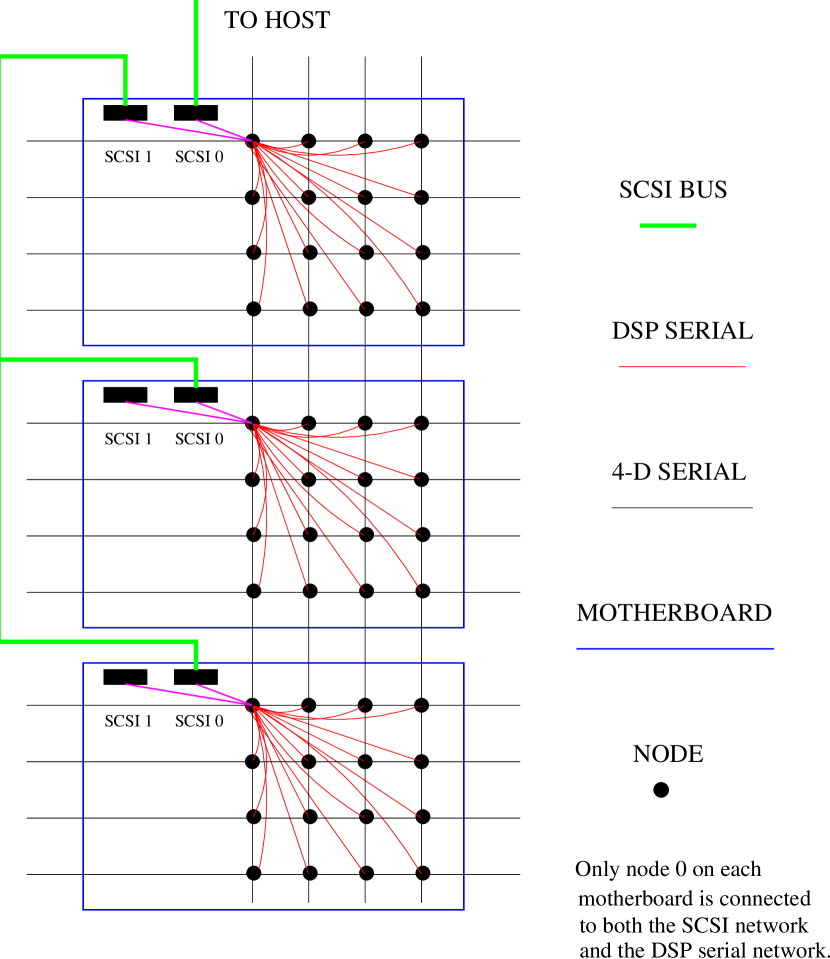
Figure 2: Networks for a two-dimensional slice of QCDSP, where 16 processing nodes are shown for a motherboard.

Node 0 on each motherboard is equivalent to all the others when a production physics calculation is underway and I/O is not being done. In addition, each node 0 can drive a standard SCSI disk, giving a large bandwidth to disk since each SCSI bus is independent and the bandwidth adds.

3.3 QCDSP Architecture: Crates and Racks

The low power of the DSP allows for close packing of the daughterboards, without having to use more than forced air cooling. Eight motherboards fit into a crate, where the backplane of the crate provides power, the clock, the reset signal, and interrupts to the motherboards. Three slots in the crate can be set to run motherboards as individual machines. Two crates (a total of 16 motherboards) fit in a rack, which is about four feet high, two feet wide and three feet deep. For pictures of the hardware, please see the Web site http://www.phys.columbia.edu/~cqft/ and links therein.

The extent of the four dimensional processor mesh is determined by ribbbon cables connected to each motherboard through the backplane. One periodic dimension of extent 4 processors is completely contained on the motherboard. The remaining three dimensions are connected with the external cables into a periodic processor mesh that is an integral multiple of $4\times 2\times 2$ in each dimension. Changing the size of the machine requires recabling and generally can be done in a few hours.

4 QCDSP Software

Another important design objective was to make QCDSP programming as straightforward as possible [10]. Although QCD algorithms are quite well established, there are continual improvements (the domain wall fermions described below are an example) and new techniques which must be added. Even leaving aside new techniques, implementing the existing body of algorithms necessary for a complete QCD simulation environment is sufficient effort that a reasonable programming environment is necessary.

One major advantage to using a commercial processor in a custom computer like QCDSP is having many software tools available. TI provides both an assembler and C compiler for the DSP. In addition, we also purchased a C++ compiler from Tartan, which has since been bought out by TI. The majority of lines of our programs are written in C++, with the kernels for the floating point intensive parts written in assembly. These are single node compilers, which do not do parallelization for the user. Also for the single node case, we have commercial debuggers, evaluation modules (commercial DSP boards hosted by a workstation or PC) and hardware emulators that we used in code development and hardware debugging. It is an enormous simplification to not be responsible for developing all these tools.

QCDSP is a fully MIMD (multiple instruction, multiple data) computer. Each processor can have a different program running on it, although this situation requires a general communication protocol running on each processor if inter-processor communication is required by the programs. For lattice gauge theory simulations, the same program is loaded to each processor with conditional branching depending on the processor coordinates in the four-dimensional processor grid.

4.1 Operating System

The QCDSP operating system was written completely at Columbia. Since the memory per processor is limited, it was not possible to consider porting Linux, for example, to QCDSP. In addition, our application does not require a full multitasking operating system, since whenever the machine is doing a physics calculation, that is all it is doing. Also, in its high performance mode, the circular buffer state is altered by interrupts. Therefore, a multitasking operating system which insisted on occasionally tending to its own housekeeping chores, would have to be switched to a non-multitasking mode during high-performance parts of the QCD programs. It is also much easier to debug hardware if the software is not throwing interrupts at random times.

In order to preserve ease of programming, the operating system provides a UNIX-like environment to a C or C++ programmer. Many standard C library calls are implemented (printf, fopen, fclose, …). (We have not implemented the C++ iostreams system at this time.) In addition, there are system calls to functions which return the grid coordinates for a processor, check the hardware status of the local processor, return the machine size, etc. Other system calls handle data transfers over the nearest neighbor network. We did not implement MPI (message passing interface), since our hardware directly supports only a subset of MPI calls. It would not be very difficult to port MPI to QCDSP.

There are two major components to the operating system. One part resides on the host SUN workstation and other runs on QCDSP. When QCDSP is booted, the host begins to query the machine and determines the total number of motherboards, daughterboards and the four-dimensional configuration of the machine. Recabling the machine does not require any software changes; the new configuration is determined on the subsequent boot. During this process, the host builds the appropriate tables which it uses to route information to any particular node.

The operating system also contains a number of features for testing and locating faulty hardware. While booting QCDSP the host does various hardware tests to determine whether there are any problems with the machine. In particular, the QCDSP run-time kernels are not loaded until the local nodes have passed a DRAM test. It is very important that the operating system be able to do a substantial amount of diagnostic work automatically on a machine with so many nodes.

When user code begins executing, the host workstation becomes a slave to QCDSP, providing services as QCDSP requests them. Currently, users have access to the host file system from QCDSP and can send output to the host console from QCDSP. More features are planned, including the QCDSP disk system. During program execution, system calls can be made to determine whether any hardware errors have occurred (parity errors on SCU transfers, single or double bit errors in data read from DRAM). At the end of user program execution, the operating system scans the machine to check the hardware state.

The operating system currently uses about 1/4 of the available memory per node. About half of this is used for buffers to store the operating system log and the results of users printf(…) calls on each node. Users can retrieve detailed information about their program from each node by retrieving the print buffer contents after program completion.

4.2 Application Software

Over the last several years, a large lattice QCD software package for QCDSP has been written in C++ and assembly. The vast majority of code is in C++, with the implementation of the various lattice Dirac operators written in assembly, along with SU(3) matrix and vector routines. Interprocessor communication is done by a set of library routines which handle the normal transfers required in lattice QCD.

While QCDSP was being built, programs to solve the Dirac equation for Wilson and staggered fermions were written. These programs were used to test the NGA design and are used as tests on the silicon wafers when NGAs are made. Our Wilson and staggered fermion inverters sustain between 20 and 30% of peak speed depending on the local volume. Now that we have a quite complete implementation of algorithms for lattice QCD, we plan to spend more time on the Dirac equation solvers. Performance between 40 and 50% is achievable.

C++ has proved very useful for organization of this fairly large software system. The C++ class structure is used, for example, to guarantee that the correct conjugate gradient solver is called for the kind of fermions you are currently working with. With around 10 collaborators working on the Columbia QCDSP machine and these 10 plus another 8 working on the RIKEN-BNL QCDSP machine, we need software organization to be able to effectively share code written by others.

Generic C++ code runs at the few percent level on QCDSP. This is primarily due to low memory bandwidth when program instructions and data are being accessed from different areas of memory. These kinds of accesses are slowed by the delays suffered when one changes DRAM pages. Function calls are also slow for similar reasons, since pushing(popping) register contents onto the stack requires writing(reading) to(from) DRAM.

QCDSP is a general computer that has been optimized for lattice QCD. There should be other grid based problems which would work well on this architecture. A completely different physics calculation has been done on QCDSP [12] and other applications are being considered.

5 QCDSP Status

The QCDSP machine at Columbia was finished in April, 1998. It has now been running production physics calculations for about a year. During the first few months of running, we removed processors which logged occasional hardware errors (primarily parity errors on SCU transfers or DRAM access). There were also nodes which would cause the machine to hang. Since the communication between each node is independent of all others, if one communication transaction does not complete, eventually all other processors will stop as the effects of the one frozen link cause successive neighbors to stall waiting for data to arrive. These kinds of errors are generally tackled by keeping a running log of the state of each link in DRAM, so that after a hang the offending link can be determined.

The RIKEN-BNL 0.6 Teraflops QCDSP machine was completed in October, 1998 and most of it has been in production running since then. We are finding the burn in time for this machine comparable to the QCDSP machine at Columbia. We expect the entire machine to be running production physics very soon. This machine was awared the Gordon Bell prize in the performance per dollar category at SC ’98 in Orlando, Florida.

6 Domain Wall Fermion Physics from QCDSP

As mentioned above, during the development of QCDSP a new lattice Dirac operator was developed, the domain wall fermion operator. The original idea was due to Kaplan [2] and was pursued by Shamir [3] and Neuberger and Narayanan [4]. Here we discuss the boundary variant of domain wall fermions due to Shamir.

When the continuum Dirac operator is discretized, one can easily change some of its properties. In particular, until recently, all known discretizations destroyed the chiral symmetry of the Dirac operator. (The chiral symmetries return as the lattice spacing is taken small, provided the parameters are adjusted appropriately.) In the continuum, chiral symmetry says that the Dirac operator does not couple left- and right-handed quarks to each other. (Handedness refers to whether the spin and momentum are parallel or antiparallel.) For massless quarks in the continuum, the left- and right- handed components only couple through the dynamics of QCD, a process known as chiral symmetry breaking.

If the discretized Dirac operator breaks chiral symmetry, then it is hard to separate the chiral symmetry breaking due to QCD and that due to the discretization. Chiral symmetry breaking is one of the dominant characteristics of the theory at low energies and it is important to have its effects clearly represented. Domain wall fermions are a discretization which preserves the chiral symmetry of the theory at finite lattice spacing,

Domain wall fermions employ a five-dimensional fermionic field, coupled to the four-dimensional gauge (gluon) field. The boundary conditions at each end of the fifth dimension are chosen so that a surface state (a mode that propagates in four dimensions) appears which is chiral. In particular, a right-handed, four dimensional quark appears at one end of the fifth dimension and a left-handed four dimensional quark at the other. These states are the four dimensional chiral quarks we desire. As the extent of the fifth dimension, $L_{s}$, is taken large, the domain wall Dirac operator breaks chiral symmetry with terms of order $\exp(-\alpha L_{s})$ where $\alpha$ is a constant.

Computationally, domain wall fermions cost a factor of $L_{s}$ more than other approaches. Simulations done by the Columbia group and others show that for smaller lattice spacing, $L_{s}=16$ is likely sufficient, while at larger lattice spacing, $L_{s}=32$ or more may be necessary. How much one gains from having chiral symmetry must be balanced against this additional cost.

6.1 QCD Thermodynamics

When QCD is heated up, the quarks and gluons which compose hadronic matter are liberated into a quark-gluon plasma. Lattice simulations have found this temperature to be $\sim 160$ MeV. However, the detailed properties of the phase transition are expected to be controlled by the symmetries of the theory, including the chiral symmetries. Since domain wall fermions have the correct chiral symmetries even at finite lattice spacing, it is important to see if our understanding of the critical region of the QCD phase transition changes with this formulation.

The group at Columbia has been actively studying the finite temperature QCD phase transition with domain wall fermions using QCDSP [13]. At the large lattice spacings where current thermodynamics studies can be done, large values for $L_{s}$ are required. Figure 3 shows the dependence on the length of the fifth dimension of the chiral condensate. (The chiral condensate should go to zero with the quark mass in the quark-gluon phase and be non-zero in the normal hadronic phase.) One can see the expected exponential fall-off for the $L_{s}$ dependent effects.

Figure 3: Dependence of the chiral condensate versus $L_{s}$ for $8^{3}\times 4$ lattices above (lower curve) and below (upper curve) the critical temperature.

We have done first simulations of the phase transition region for QCD using domain wall fermions and $L_{s}=24$. This is not a large enough value for $L_{s}$ to completely remove the exponentially small chiral symmetry breaking effects. However, we did find the temperature for the QCD phase transition with domain wall fermions to be $\sim 170$ MeV, which is consistent with other techniques. We are currently doing more simulations with smaller chiral symmetry breaking effects. The power of the QCDSP computers is vital for these studies.

6.2 Weak Matrix Elements

Part of testing the standard model of particle physics involves knowing precisely the effects of weak interactions on hadronic states. We must use computational techniques to make the hadrons and then measure the weak interaction effects in these hadrons made on the computer. The process of inserting the weak interaction effects into the hadrons is much more controlled if chiral symmetry is intact. Without chiral symmetry, different effects can become intermixed. In addition, chiral symmetry tells us that the behavior of weak interactions in certain hadronic states becomes small as the quark mass becomes small. Without chiral symmetry to enforce this condition, one ends up calculating a small number by subtracting two large numbers. This is very costly and introduces large errors.

In the realm of weak interactions in QCD systems, the topic of CP violation is of particular importance. The standard model allows the combined symmetry of charge conjugation and parity (CP symmetry) to be violated, due to the presence of one complex parameter in the theory. CP violation was first measured experimentally in 1964 by Cronin and Fitch in the kaon system (the kaon is a bound state of two quarks, one of which is the strange quark). This measurement of CP violation through what is called mixing has recently been joined by a new experimental announcement of CP violation in decays. Without detailed QCD calculations, one cannot know if both effects are consistent with a single value for the complex parameter in the standard model.

The first work on weak matrix elements with domain wall fermions was done by [14] who calculated a parameter related to CP violation by mixing for quenched QCD. (This had previously been done by other groups using Wilson and staggered fermions.) They found that for moderately small lattice spacings, an $L_{s}$ of $\sim 16$ effectively restored chiral symmetry for the domain wall fermions. In a joint work using the QCDSP computer at the RIKEN-BNL Research Center, a collaboration of the RIKEN-BNL, BNL and Columbia lattice groups (which includes the authors of [14]) are using domain wall fermions to calculate the CP violation in mixing and decays, for quenched QCD.

CP violation in decays has been worked on for some time using other fermions formulations. The lack of the full symmetries of the theory has made these calculations very difficult, a problem which is solved by the domain wall fermions. The domain wall fermions make the calculation many times more computationally expensive, but may solve enough other problemss that a final answer is possible. We are anxiously awaiting the completion of this calculation.

7 Conclusions

The QCDSP computer is a very cost effective computer for calculations in lattice QCD. This computer was designed and constructed by a small group of people, primarily physicists, over five years with a total parts cost of $\sim 4$ million dollars, including research and development. (Salaries add an additional $\sim 1.5$ million dollars to the cost.) The final machine has a cost performance of about $10/Megaflops and won the 1998 Gordon Bell prize in the cost performance category at SC ’98 in Orlando, Florida.

Including the Columbia and RIKEN-BNL computers, 20,480 processors with a peak speed of over 1 Teraflops are available for QCD calculations. Physicists at Columbia, BNL and RIKEN-BNL are aggressively using these machines to study QCD, focusing on using the new domain wall fermion formalism. Calculations for QCD thermodynamics and weak matrix elements, among others, are well underway.

Acknowledgements

The QCDSP computer was developed with funds provided by the United States Department of Energy. Funds for the 0.4 Teraflops QCDSP computer were provided by the US DOE, while the 0.6 Teraflops computer was funded by the RIKEN-BNL Research Center. The work discussed here is the cumulative effort of many individuals over a number of years. They are:

Columbia University:

Current Members:

Ping Chen, Norman Christ, George Fleming, Tim Klassen, Robert Mawhinney, Gabi Siegert, ChengZhong Sui, Pavlos Vranas, Lingling Wu and Yuri Zhestkov.

Former Members:

Igor Arsenin, Dong Chen, Chulwoo Jung, Adrian
Kaehler, Yubing Luo and Catalin Malureanu.

Columbia University Nevis Laboratories:

Alan Gara and John Parsons

Brookhaven National Laboratory:

Michael Creutz, Chris Dawson and
Amarjit Soni.

RIKEN-BNL Research Center:

Tom Blum, Shigemi Ohta, Shoichi Sasaki and Matthew Wingate

SCRI at Florida State:

Robert Edwards and Tony Kennedy (now at Edinburgh)

The Ohio State University:

Greg Kilcup

Trinity College, Dublin:

Jim Sexton

Fermilab:

Sten Hanson

References

- [1] Two textbooks on lattice gauge theory are Quarks, gluons and lattices by Michael Creutz, Cambridge, 1983 and Quantum fields on a lattice by Istvan Montvay and Gernot Munster, Cambridge, 1994.
- [2] D. Kaplan, Physics Letters B 288 (1992) 342.
- [3] Y. Shamir, Nuclear Physics B 406 (1993) 90, V. Furman and Y. Shamir, Nuclear Physics 439 (1995) 54.
- [4] R. Narayanan and H. Neuberger, Nuclear Physics B 443 (1995) 305. See also references in the article Chiral Fermions on the Lattice in this volume.
- [5] I. Arsenin, et. al., Nuclear Physics B (Proc. Suppl.) 34 (1994) 820.
- [6] Y. Iwasaki, et. al., Nuclear Physics B (Proc. Suppl.) 34 (1994) 78.
- [7] R. Mawhinney, Nuclear Physics B (Proc. Suppl.) 42 (1995) 140.
- [8] I. Arsenin, et. al., Nuclear Physics B (Proc. Suppl.) 47 (1996) 804.
- [9] R. Mawhinney, Nuclear Physics B (Proc. Suppl.) 53 (1997) 1010.
- [10] R. Edwards, et. al., Nuclear Physics B (Proc. Suppl.) 63A-C (1998) 997.
- [11] Michael Creutz, private communication.
- [12] M. Creutz, Grassmann integrals by machine, hep-lat/9809024.
- [13] P. Chen, et. al., CU-TP-914, hep-lat/9809159, P. Vranas, hep-lat/9903024.
- [14] T. Blum and A. Soni, Physical Review Letters, 79 (1997) 3595.