Cost of Generalised HMC Algorithms for Free Field Theory

Abstract

We study analytically the computational cost of the Generalised Hybrid Monte Carlo (GHMC) algorithm for free field theory. We calculate the autocorrelation functions of operators quadratic in the fields, and optimise the GHMC momentum mixing angle, the trajectory length, and the integration stepsize. We show that long trajectories are optimal for GHMC, and that standard HMC is much more efficient than algorithms based on the Second Order Langevin (L2MC) or Kramers Equation. We show that contrary to naive expectations HMC and L2MC have the same volume dependence, but their dynamical critical exponents are $z=1$ and $z=3/2$ respectively.

1 GENERALISED HMC

The work reported here extends results presented previously [1, 2], to which the reader is referred for details. We begin by recalling that the generalised HMC [2] algorithm is constructed from two kinds of update for a set of fields $\phi$ and their conjugate momenta $\pi$.

Molecular Dynamics Monte Carlo: This consists of three parts: (1) MD: an approximate integration of Hamilton’s equations on phase space which is exactly area-preserving and reversible; $U(\tau):(\phi,\pi)\mapsto(\phi^{\prime},\pi^{\prime})$ where $\det U=1$ and $U(\tau)=U(-\tau)^{-1}$. (2) A momentum flip $F:\pi\mapsto-\pi$. (3) MC: a Metropolis accept/reject test.

Partial Momentum Refreshment: This mixes the Gaussian-distributed momenta $\pi$ with Gaussian noise $\xi$:

$$\left(\begin{array}[]{c}\pi^{\prime}\\ \xi^{\prime}\end{array}\right)=\left(\begin{array}[]{cc}\cos\vartheta&\sin\vartheta\\ -\sin\vartheta&\cos\vartheta\end{array}\right)\cdot F\left(\begin{array}[]{c}\pi\\ \xi\end{array}\right)$$

The HMC algorithm [3] is the special case where $\vartheta={\pi\over 2}$. The L2MC/Kramers algorithm [4, 5] corresponds to choosing arbitrary $\vartheta$ but MDMC trajectories of a single leapfrog integration step.

1.1 Tunable Parameters

The GHMC algorithm has three free parameters, the trajectory length $\tau$, the momentum mixing angle $\vartheta$, and the integration step size ${\delta\tau}$. These may be chosen arbitrarily without affecting the validity of the method, except for some special values for which the algorithm ceases to be ergodic. We may adjust these parameters to minimise the cost of a Monte Carlo computation, and the main goal of this work is to carry out this optimisation procedure for free field theory.

Horowitz pointed out that the L2MC algorithm has the advantage of having a higher acceptance rate than HMC for a given step size, but he did not take in to account that it also requires a higher acceptance rate to get the same autocorrelations because the trajectory is reversed at each MC rejection. It is not obvious a priori which of these effects dominates.

The parameters $\tau$ and $\vartheta$ may be chosen independently from some distributions $P_{R}(\tau)$ and $P_{M}(\vartheta)$ for each trajectory. In the following we shall consider various choices for the momentum refreshment distribution $P_{M}$, but we shall always take a fixed value for $\vartheta$.

2 FREE FIELD THEORY

Consider a system of harmonic oscillators $\{\phi_{p}\}$ for $p\in{\twelvebb Z}_{V}$. The Hamiltonian on phase space is $H={1\over 2}\sum_{p\in{\twelvebb Z}_{V}}\left(\pi_{p}^{2}+\omega_{p}^{2}\phi^{2}\right)$. This describes free field theory in momentum space if the frequencies $\omega_{p}$ are chosen as

$$\omega_{p}^{2}=m^{2}+4\sum_{\mu=1}^{d}\sin^{2}\frac{\pi p_{\mu}}{L}.$$ (1)

3 AUTOCORRELATION FUNCTIONS

3.1 Simple Markov Processes

Let $(\phi_{1},\phi_{2},\ldots,\phi_{N})$ be a sequence of field configurations generated by an equilibrated ergodic Markov process, and let $\langle\Omega(\phi)\rangle$ denote the expectation value of some connected operator $\Omega$. We may define an unbiased estimator $\bar{\Omega}$ over the finite sequence of configurations by $\bar{\Omega}\equiv{1\over N}\sum_{t=1}^{N}\Omega(\phi_{t})$, As usual, we define $C_{\Omega}(\ell)\equiv{\bigl{\langle}\Omega(\phi_{t}+\ell)\Omega(\phi_{t})\bigr{\rangle}\over\bigl{\langle}\Omega(\phi)^{2}\bigr{\rangle}}$ as the autocorrelation function for $\Omega$. The variance of the estimator $\bar{\Omega}$ is

$$\langle{\bar{\Omega}}^{2}\rangle=\{1+2A_{\Omega}\}{\bigl{\langle}\Omega(\phi)^{2}\bigr{\rangle}\over N}\left[1+O\left({{{N}_{\hbox{\rm\tiny exp}}}\over N}\right)\right],$$

where $A_{\Omega}\equiv\sum_{\ell=1}^{\infty}C_{\Omega}(\ell)$ is the integrated autocorrelation function for the operator $\Omega$ and ${{N}_{\hbox{\rm\tiny exp}}}$ is the exponential autocorrelation time. This result tells us that on average $1+2A_{\Omega}$ correlated measurements are needed to reduce the variance by the same amount as a single truly independent measurement.

3.2 Autocorrelation Functions for Quadratic Operators

In order to carry out these calculations we make the simplifying assumption that the acceptance probability $\min\bigl{(}1,e^{-{\delta H}}\bigr{)}$ for each trajectory may be replaced by its value averaged over phase space ${{P}_{\hbox{\rm\tiny acc}}}\equiv\left\langle\min\bigl{(}1,e^{-{\delta H}}\bigr{)}\right\rangle$; we neglect correlations between successive trajectories. Including such correlations leads to seemingly intractable complications. It is not obvious that our assumption corresponds to any systematic approximation except, of course, that it is valid when ${\delta H}=0$.

Details of the calculation of ${{P}_{\hbox{\rm\tiny acc}}}$ for leapfrog integration are published elsewhere [1, 2, 6].

4 COMPARISON OF COSTS

If we make the reasonable assumption that the cost of the computation is proportional to the total fictitious (MD) time for which we have to integrate Hamilton’s equations, then the cost ${\twelvefk C}$ per independent configuration is proportional to $(1+2A_{\Omega}){\bar{\tau}}/{\delta\tau}$ with ${\bar{\tau}}$ denoting the average length of a trajectory. The optimal trajectory length is obtained by minimising the cost, that is by choosing ${\bar{\tau}}$ so as to satisfy ${d{\twelvefk C}/d{\bar{\tau}}}={d{\twelvefk C}/d\vartheta}=0$.

We wish to compare the performance of the HMC, L2MC and GHMC algorithms for one dimensional free field theory. To do this we compare the cost of generating a statistically independent measurement of the magnetic susceptibility $M^{2}_{c}$, choosing the optimal values for the angle $\vartheta$ and the average trajectory length ${\bar{\tau}}$. We can minimise the cost with respect to $\vartheta$ without having to specify the form of the refresh distribution.

The next step is to minimise the cost with respect to the average trajectory length $\xi=\omega{\bar{\tau}}$. Strictly speaking we should note that the acceptance probability ${{\bar{P}}_{\hbox{\rm\tiny acc}}}$ is a function of ${\bar{\tau}}$, but to a good approximation we may assume that ${{P}_{\hbox{\rm\tiny acc}}}$ depends only upon the integration step size ${\delta\tau}$ except in the case of very short trajectories.

4.1 Exponentially Distributed Trajectory Lengths

To proceed further we need to choose a specific form for the momentum refresh distribution. In this section we will present results for the case of exponentially distributed trajectory lengths, $P_{R}(\tau)=re^{-r\tau}$ where the parameter $r$ is just the inverse average trajectory length $r=1/{\bar{\tau}}$.

The cost at the point $({{c}_{\hbox{\rm\tiny opt}}}\equiv\cos{{\vartheta}_{\hbox{\rm\tiny opt}}},{{\xi}_{\hbox{\rm\tiny opt}}})$ is

$${\twelvefk C}^{\hbox{\tiny exp}}_{M^{2}_{c}}({\delta\tau},{{\vartheta}_{\hbox{\rm\tiny opt}}},{{\xi}_{\hbox{\rm\tiny opt}}})~{}=~{}$$

$$\frac{\left(\begin{array}[]{c}(7{{\bar{P}}_{\hbox{\rm\tiny acc}}}-3{{\bar{P}}_{\hbox{\rm\tiny acc}}}^{2}-4){{\xi}_{\hbox{\rm\tiny opt}}}^{2}{{c}_{\hbox{\rm\tiny opt}}}^{3}+1-{{c}_{\hbox{\rm\tiny opt}}}^{2}\\ {}+(-2{{\bar{P}}_{\hbox{\rm\tiny acc}}}+1){{c}_{\hbox{\rm\tiny opt}}}+(2{{\bar{P}}_{\hbox{\rm\tiny acc}}}-1){{c}_{\hbox{\rm\tiny opt}}}^{3}\\ {}+({{\bar{P}}_{\hbox{\rm\tiny acc}}}^{2}-5{{\bar{P}}_{\hbox{\rm\tiny acc}}}+4){{c}_{\hbox{\rm\tiny opt}}}{{\xi}_{\hbox{\rm\tiny opt}}}^{2}\\ {}+(-{{\bar{P}}_{\hbox{\rm\tiny acc}}}+4){{\xi}_{\hbox{\rm\tiny opt}}}^{2}+(-4+3{{\bar{P}}_{\hbox{\rm\tiny acc}}}){{c}_{\hbox{\rm\tiny opt}}}^{2}{{\xi}_{\hbox{\rm\tiny opt}}}^{2}\end{array}\right)}{\left(\begin{array}[]{c}{{\bar{P}}_{\hbox{\rm\tiny acc}}}{\delta\tau}\omega({{\bar{P}}_{\hbox{\rm\tiny acc}}}-1){{c}_{\hbox{\rm\tiny opt}}}^{3}{{\xi}_{\hbox{\rm\tiny opt}}}\\ {}+{{\xi}_{\hbox{\rm\tiny opt}}}{{\bar{P}}_{\hbox{\rm\tiny acc}}}{\delta\tau}\omega-{{\xi}_{\hbox{\rm\tiny opt}}}{{\bar{P}}_{\hbox{\rm\tiny acc}}}{\delta\tau}\omega{{{c}_{\hbox{\rm\tiny opt}}}}^{2}\\ {}-{{\bar{P}}_{\hbox{\rm\tiny acc}}}{\delta\tau}\omega(-1+{{\bar{P}}_{\hbox{\rm\tiny acc}}}){{c}_{\hbox{\rm\tiny opt}}}{{\xi}_{\hbox{\rm\tiny opt}}}\end{array}\right)}\,.$$

This solution is a function of ${\delta\tau}$ and ${{\bar{P}}_{\hbox{\rm\tiny acc}}}$ which are not independent variables, and using the results for ${{\bar{P}}_{\hbox{\rm\tiny acc}}}(\tau,{\delta\tau})$ [1, 2] we can compute the cost as a function of ${{\bar{P}}_{\hbox{\rm\tiny acc}}}$ as shown in Figure 1.

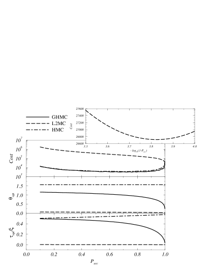
Figure 1: Cost as a function of average Metropolis acceptance rate for the GHMC algorithm compared to HMC and L2MC for free field theory. The operator under consideration is the “magnetic susceptibility”, i.e., the connected quadratic operator depending only on the lowest frequency mode. The corresponding parameters, the momentum mixing angle $\vartheta_{\mathop{\rm opt}}$ and the average trajectory length measured as a fraction of the correlation length $\tau_{\mathop{\rm opt}}/\xi$ are also shown, all as a function of the acceptance rate ${{\bar{P}}_{\hbox{\rm\tiny acc}}}$. The inset graph shows the region where the acceptance rate is very close to unity which is where the L2MC algorithm has its minimum cost.

4.1.1 HMC

The Hybrid Monte Carlo algorithm corresponds to setting $\vartheta=\pi/2$, and we find that the optimal trajectory length in this case is ${{\xi}_{\hbox{\rm\tiny opt}}}=1/\sqrt{4-{{\bar{P}}_{\hbox{\rm\tiny acc}}}}$, corresponding to a cost

$${{{\twelvefk C}}_{\hbox{\rm\tiny opt}}}={2\sqrt{4-{{\bar{P}}_{\hbox{\rm\tiny acc}}}}\over{{\bar{P}}_{\hbox{\rm\tiny acc}}}{\delta\tau}\omega}.$$

This is also shown in Figure 1.

4.2 Fixed Length Trajectories

For fixed length trajectories we shall only analyse the case of L2MC for which the trajectory length $\xi=\omega{\delta\tau}$. In this case the value of ${{\vartheta}_{\hbox{\rm\tiny opt}}}$ and the corresponding cost are also plotted in Figure 1. From this figure it is clear that the minimum cost occurs for ${{\bar{P}}_{\hbox{\rm\tiny acc}}}$ very close to unity, where the scaling variable $x=V{\delta\tau}^{6}$ is very small. We may then express ${{c}_{\hbox{\rm\tiny opt}}}$ and ${{\bar{P}}_{\hbox{\rm\tiny acc}}}$ as power series in $x$, keeping only the first few terms. From these relations we find that the minimum cost for L2MC is

$${{{\twelvefk C}}_{\hbox{\rm\tiny opt}}}=\left(10\over\pi\right)^{1/4}V^{5/4}m^{-3/2}.$$

This result tells us that not only does the tuned L2MC algorithm have a dynamical critical exponent $z=3/2$, but also it has a volume dependence of exactly the same form as HMC [1, 2]. We may understand why this behaviour occurs rather than the naive $V^{7/6}m^{-1}$ by the following simple argument.

If ${{\bar{P}}_{\hbox{\rm\tiny acc}}}<1$ then the system will carry out a random walk backwards and forwards along a trajectory because the momentum, and thus the direction of travel, must be reversed upon a Metropolis rejection. A simple minded analysis is that the average time between rejections must be $O(1/m)$ in order to achieve $z=1$. This time is approximately

$$\sum_{n=0}^{\infty}{{\bar{P}}_{\hbox{\rm\tiny acc}}}^{n}(1-{{\bar{P}}_{\hbox{\rm\tiny acc}}})n{\delta\tau}={{{\bar{P}}_{\hbox{\rm\tiny acc}}}{\delta\tau}\over 1-{{\bar{P}}_{\hbox{\rm\tiny acc}}}}={1\over m}.$$

For small ${\delta\tau}$ we have $1-{{\bar{P}}_{\hbox{\rm\tiny acc}}}=\mathop{\rm erf}\sqrt{kV{\delta\tau}^{6}}\propto\sqrt{V{\delta\tau}^{6}}$ where $k$ is a constant, and hence we must scale ${\delta\tau}$ so as to keep $V{\delta\tau}^{4}/m^{2}$ fixed. Since the L2MC algorithm has a naive dynamical critical exponent $z=1$, this means that the cost should vary as ${\twelvefk C}\propto V(V{\delta\tau}^{4}m^{-2})^{1/4}/m{\delta\tau}=V^{5/4}m^{-3/2}$.

References

[1]A. D. Kennedy and B. J. Pendleton,
Nucl. Phys. B (Proc. Suppl.) 20 (1991) 118.
[2]
A. D. Kennedy, R. G. Edwards, H. Mino, and B. J. Pendleton,
Nucl. Phys. B (Proc. Suppl.) 47 (1995) 781.
[3]
S. Duane, A. D. Kennedy, B. J. Pendleton, and D. Roweth,
Phys. Lett. 195B (1987) 216.
[4]
A. M. Horowitz,
Phys. Lett. B268 (1991) 247.
[5]
M. Beccaria and G. Curci,
Phys. Rev. D49 (1994) 2578.
[6]
A. D. Kennedy and B. J. Pendleton, in preparation.