Perturbative Renormalization Factors of Baryon Number Violating Operators for Improved Quark and Gauge Actions in Lattice QCD

Abstract

We calculate one-loop renormalization factors of three-quark operators, which appear in the low energy effective Lagrangian of the nucleon decay, for $O(a)$-improved quark action and gauge action including six-link loops. This calculation is required to predict the hadronic nucleon decay matrix elements in the continuum regularization scheme using lattice QCD. We present detailed numerical results of the one-loop coefficients for general values of the clover coefficients employing the several improved gauge actions in the Symanzik approach and in the Wilson’s renormalization group approach. The magnitudes of the one-loop coefficients for the improved gauge actions show sizable reduction compared to those for the plaquette action.

I Introduction

While nucleon decay is one of the most exciting prediction from grand unified theories (GUTs) with and without supersymmetry, none of the decay modes have been experimentally detected up to now. Furthermore, the ongoing Super-Kamiokande experiment is now pushing the lower limit on the partial lifetimes of the nucleon by an order of magnitude from the previous measurements. In principle this would give a strong constraint on (SUSY-)GUTs, however, the uncertainties in the theoretical prediction of lifetimes due to poor knowledge of quantum effects at low energy such as hadron or SUSY scales obscure the direct impact of the experimental lifetime bound on the physics at the GUT scale. In particular, one of the main uncertainties has been found in the evaluation of the hadron matrix elements for the nucleon decays, for which various QCD models have given estimate differing by a factor of ten. Therefore precise determination of the nucleon decay matrix elements from first principles is required, for which Lattice QCD can play a crucial role.

Recently we carried out a model-independent calculation of the nucleon decay matrix elements employing the Wilson quark action and the plaquette gauge action in the quenched approximation[1]. Although one naively expects the error in the discretization and quenching approximation which are the two main systematic errors, it would be desirable to reduce these unknown systematic errors for high precision calculation. As a step toward this goal we are required to reduce the scaling violation effects by improving quark and gauge actions. In this article we present perturbative results for renormalization factors of baryon number violating operators for improved quark and gauge actions: the $O(a)$-improved “clover” action originally proposed by Sheikholeslami and Wohlert[2] and the gauge action improved by addition of six link loops to the plaquette term in the Symanzik approach[3] and in the Wilson’s renormalization group approach[4, 5]. Values of the one-loop coefficients of the renormalization factors are numerically evaluated for combinations of general values of the clover coefficients in the quark action and some specific values of the coefficients of the six-link loop terms in the gauge action.

This paper is organized as follows. In Sec.II we give the improved quark and gauge actions on the lattice and their Feynman rules relevant for their calculation. Our calculational procedure of the renormalization factors for the baryon number violating operators is described in Sec.III, where we present expressions and numerical values for the one-loop coefficients of the renormalization factors. Our conclusions are summarized in Sec.IV.

The physical quantities are expressed in lattice units, and the lattice spacing $a$ is suppressed unless necessary. Throughout this paper we use the same notation for quantities defined on the lattice and their counterparts in the continuum. In case of any possibility of confusion, however, we shall make a clear distinction between them.

II Actions and Feynman rules

For the gauge action we consider the following general form including the standard plaquette term and six-link loop terms:

$$S_{\rm gauge}=\frac{1}{g^{2}}\left\{c_{0}\sum_{\rm plaquette}{\rm Tr}U_{pl}+c_{1}\sum_{\rm rectangle}{\rm Tr}U_{rtg}+c_{2}\sum_{\rm chair}{\rm Tr}U_{chr}+c_{3}\sum_{\rm parallelogram}{\rm Tr}U_{plg}\right\}$$ (1)

with the normalization condition

$$c_{0}+8c_{1}+16c_{2}+8c_{3}=1,$$ (2)

where six-link loops are $1\times 2$ rectangle, a bent $1\times 2$ rectangle (chair) and a three-dimensional parallelogram obtained by multiplying the link variables

$$U_{n,\mu}={\rm exp}\left(ig\sum_{a}T^{a}A_{\mu}^{a}(n+{\hat{\mu}}/{2})\right).$$ (3)

The free gluon propagator is obtained in Ref.[3]:

$$D_{\mu\nu}(k)=\frac{1}{({\hat{k}}^{2})^{2}}\left[(1-A_{\mu\nu}){\hat{k}}_{\mu}{\hat{k}}_{\nu}+\delta_{\mu\nu}\sum_{\sigma}{\hat{k}}_{\sigma}^{2}A_{\nu\sigma}\right]$$ (4)

with

$${\hat{k}}_{\mu} = 2{\rm sin}\left(\frac{k_{\mu}}{2}\right),$$ (5)

$${\hat{k}}^{2} = \sum_{\mu=1}^{4}{\hat{k}}_{\mu}^{2}.$$ (6)

The matrix $A_{\mu\nu}$ satisfies

$$({\rm i}) A_{\mu\mu}=0\;\;\;{\rm for}\;\;{\rm all}\;\;\mu,$$ (7)

$$({\rm ii}) A_{\mu\nu}=A_{\nu\mu},$$ (8)

$$({\rm iii}) A_{\mu\nu}(k)=A_{\mu\nu}(-k).$$ (9)

$$({\rm iv}) A_{\mu\nu}(0)=1\;\;\;{\rm for}\;\;\mu\neq\nu,$$ (10)

and its expression is given by

$$A_{\mu\nu}(k) = \frac{1}{\Delta_{4}}\left[({\hat{k}}^{2}-{\hat{k}}_{\nu}^{2})(q_{\mu\rho}q_{\mu\tau}{\hat{k}}_{\mu}^{2}+q_{\mu\rho}q_{\rho\tau}{\hat{k}}_{\rho}^{2}+q_{\mu\tau}q_{\rho\tau}{\hat{k}}_{\tau}^{2})\right.$$ (15)

$$\left.+({\hat{k}}^{2}-{\hat{k}}_{\mu}^{2})(q_{\nu\rho}q_{\nu\tau}{\hat{k}}_{\nu}^{2}+q_{\nu\rho}q_{\rho\tau}{\hat{k}}_{\rho}^{2}+q_{\nu\tau}q_{\rho\tau}{\hat{k}}_{\tau}^{2})\right.$$

$$\left.+q_{\mu\rho}q_{\nu\tau}({\hat{k}}_{\mu}^{2}+{\hat{k}}_{\rho}^{2})({\hat{k}}_{\nu}^{2}+{\hat{k}}_{\tau}^{2})+q_{\mu\tau}q_{\nu\rho}({\hat{k}}_{\mu}^{2}+{\hat{k}}_{\tau}^{2})({\hat{k}}_{\nu}^{2}+{\hat{k}}_{\rho}^{2})\right.$$

$$\left.-q_{\mu\nu}q_{\rho\tau}({\hat{k}}_{\rho}^{2}+{\hat{k}}_{\tau}^{2})^{2}-(q_{\mu\rho}q_{\nu\rho}+q_{\mu\tau}q_{\nu\tau}){\hat{k}}_{\rho}^{2}{\hat{k}}_{\tau}^{2}\right.$$

$$\left.-q_{\mu\nu}(q_{\mu\rho}{\hat{k}}_{\mu}^{2}{\hat{k}}_{\tau}^{2}+q_{\mu\tau}{\hat{k}}_{\mu}^{2}{\hat{k}}_{\rho}^{2}+q_{\nu\rho}{\hat{k}}_{\nu}^{2}{\hat{k}}_{\tau}^{2}+q_{\nu\tau}{\hat{k}}_{\nu}^{2}{\hat{k}}_{\rho}^{2})\right],$$

with $\mu\neq\nu\neq\rho\neq\tau$ the Lorentz indices. $q_{\mu\nu}$ and $\Delta_{4}$ are written as

$$q_{\mu\nu} = (1-\delta_{\mu\nu})\left[1-(c_{1}-c_{2}-c_{3})({\hat{k}}_{\mu}^{2}+{\hat{k}}_{\nu}^{2})-(c_{2}+c_{3}){\hat{k}}^{2}\right],$$ (16)

$$\Delta_{4} = \sum_{\mu}{\hat{k}}_{\mu}^{4}\prod_{\nu\neq\mu}q_{\nu\mu}+\sum_{\mu>\nu,\rho>\tau,\{\rho,\tau\}\cap\{\mu,\nu\}=\emptyset}{\hat{k}}_{\mu}^{2}{\hat{k}}_{\nu}^{2}q_{\mu\nu}(q_{\mu\rho}q_{\nu\tau}+q_{\mu\tau}q_{\nu\rho}).$$ (17)

In the case of the standard plaquette action, the matrix $A_{\mu\nu}$ is simplified as

$$A_{\mu\nu}^{\rm plaquette}=1-\delta_{\mu\nu}.$$ (18)

For the quark action we consider the $O(a)$-improved quark action:

$$S_{\rm quark} = \sum_{n}\frac{1}{2}\sum_{\mu}\left\{{\bar{\psi}}_{n}(-r+\gamma_{\mu})U_{n,\mu}\psi_{n+{\hat{\mu}}}+{\bar{\psi}}_{n}(-r-\gamma_{\mu})U^{\dagger}_{n-{\hat{\mu}},\mu}\psi_{n-{\hat{\mu}}}\right\}+(m_{0}+4r)\sum_{n}{\bar{\psi}}_{n}\psi_{n}$$ (20)

$$-{c_{\rm SW}}\sum_{n}\sum_{\mu,\nu}ig\frac{r}{4}{\bar{\psi}}_{n}\sigma_{\mu\nu}P_{\mu\nu}(n)\psi_{n},$$

where we define the Euclidean gamma matrices in terms of the Minkowski matrices in the Bjorken-Drell convention: $\gamma_{j}=-i\gamma_{BD}^{j}$ $(j=1,2,3)$, $\gamma_{4}=\gamma_{BD}^{0}$, $\gamma_{5}=\gamma_{BD}^{5}$ and $\sigma_{\mu\nu}=\frac{1}{2}[\gamma_{\mu},\gamma_{\nu}]$. The field strength $P_{\mu\nu}$ in the “clover” term is given by

$$P_{\mu\nu}(n) = \frac{1}{4}\sum_{i=1}^{4}\frac{1}{2ig}\left(U_{i}(n)-U_{i}^{\dagger}(n)\right),$$ (21)

$$U_{1}(n) = U_{n,\mu}U_{n+{\hat{\mu}},\nu}U^{\dagger}_{n+{\hat{\nu}},\mu}U^{\dagger}_{n,\nu},$$ (22)

$$U_{2}(n) = U_{n,\nu}U^{\dagger}_{n-{\hat{\mu}}+{\hat{\nu}},\mu}U^{\dagger}_{n-{\hat{\mu}},\nu}U_{n-{\hat{\mu}},\mu},$$ (23)

$$U_{3}(n) = U^{\dagger}_{n-{\hat{\mu}},\mu}U^{\dagger}_{n-{\hat{\mu}}-{\hat{\nu}},\nu}U_{n-{\hat{\mu}}-{\hat{\nu}},\mu}U_{n-{\hat{\nu}},\nu},$$ (24)

$$U_{4}(n) = U^{\dagger}_{n-{\hat{\nu}},\nu}U_{n-{\hat{\nu}},\mu}U_{n+{\hat{\mu}}-{\hat{\nu}},\nu}U^{\dagger}_{n,\mu}.$$ (25)

From the quark action (20) we obtain the free quark propagator

$$S_{q}^{-1}(p)=i\sum_{\mu}\gamma_{\mu}{\rm sin}(k_{\mu})+m_{0}+r\sum_{\mu}(1-{\rm cos}(p_{\mu})).$$ (26)

In order to calculate renormalization factors of the baryon number violating operators up to one-loop level, we need the following vertices,

$$V^{a}_{1\mu}(p,q)=-igT^{a}\left\{\gamma_{\mu}{\rm cos}\left(\frac{p_{\mu}+q_{\mu}}{2}\right)-ir{\rm sin}\left(\frac{p_{\mu}+q_{\mu}}{2}\right)\right\},$$ (27)

$$V^{a}_{c1\mu}(p,q)=-gT^{a}{c_{\rm SW}}\frac{r}{2}\left(\sum_{\nu}\sigma_{\mu\nu}{\rm sin}(p_{\nu}-q_{\nu})\right){\rm cos}\left(\frac{p_{\mu}-q_{\mu}}{2}\right)$$ (28)

with $p_{\mu}$ incoming quark momentum and $q_{\mu}$ outgoing quark momentum. The first vertex originates from the Wilson quark action and the second one is the interaction due to the clover term. In the present calculation of the vertex corrections for the baryon number violating operators, the two-gluon vertices with quarks give no contribution.

We should note that the baryon number violating operators contain a charge conjugated field, whose action is obtained from eq.(20) with the replacement of

$$T^{a}\longrightarrow-(T^{a})^{T},$$ (29)

where the superscript $T$ means the transposed matrix. According to this change, the Feynman rule of the quark-gluon vertices in eqs.(27) and (28) should be modified for the charge conjugated field.

III Renormalization factors for baryon number violating operators

A Calculational procedure

We consider the following baryon number violating operators in the continuum and on the lattice:

$$\left({\cal O}_{X,Y}^{\rm cont}\right)_{\delta} = \epsilon^{abc}\left[({\bar{\psi}}_{1}^{c})^{a}\Gamma_{X}(\psi_{2})^{b}\right]\left[\Gamma_{Y}(\psi_{3})^{c}\right]_{\delta},$$ (30)

$$\left({\cal O}_{X,Y}^{\rm latt}\right)_{\delta} = \epsilon^{abc}\left[\left\{1+rm_{0}(1-z)\right\}({\bar{\psi}}_{1}^{c})^{a}\Gamma_{X}(\psi_{2})^{b}\right.$$ (34)

$$\left.+z\frac{r}{2}\left\{({\bar{\psi}}_{1}^{c}{\stackrel{{\scriptstyle\leftarrow}}{{D{/}}}})^{a}\Gamma_{X}(\psi_{2})^{b}-({\bar{\psi}}_{1}^{c})^{a}\Gamma_{X}({\stackrel{{\scriptstyle\rightarrow}}{{D{/}}}}\psi_{2})^{b}\right\}\right.$$

$$\left.-z^{2}\frac{r^{2}}{4}({\bar{\psi}}_{1}^{c}{\stackrel{{\scriptstyle\leftarrow}}{{D{/}}}})^{a}\Gamma_{X}({\stackrel{{\scriptstyle\rightarrow}}{{D{/}}}}\psi_{2})^{b}\right]$$

$$\times\left[\left\{1+\frac{r}{2}m_{0}(1-z)\right\}\Gamma_{Y}(\psi_{3})^{c}-z\frac{r}{2}\Gamma_{Y}({\stackrel{{\scriptstyle\rightarrow}}{{D{/}}}}\psi_{3})^{c}\right]_{\delta}$$

with

$${\stackrel{{\scriptstyle\rightarrow}}{{D{/}}}}\psi_{n} = \frac{1}{2}\sum_{\mu}\gamma_{\mu}\left(U_{n,\mu}\psi_{n+{\hat{\mu}}}-U^{\dagger}_{n-{\hat{\mu}},\mu}\psi_{n-\hat{\mu}}\right),$$ (35)

$${\bar{\psi}}_{n}^{c}{\stackrel{{\scriptstyle\leftarrow}}{{D{/}}}} = \frac{1}{2}\sum_{\mu}\left({\bar{\psi}}^{c}_{n+{\hat{\mu}}}U^{T}_{n,\mu}-{\bar{\psi}}^{c}_{n-\hat{\mu}}U^{\ast}_{n-{\hat{\mu}},\mu}\right)\gamma_{\mu},$$ (36)

where ${\bar{\psi}}^{c}=\psi^{T}C$ with $C=\gamma_{4}\gamma_{2}$ is a charge conjugated field of $\psi$. Dirac structures are represented by $\Gamma_{X}\otimes\Gamma_{Y}=P_{R}\otimes P_{R},P_{R}\otimes P_{L},P_{L}\otimes P_{R},P_{L}\otimes P_{L}$ with the right- and left-handed projection operators $P_{R,L}=(1\pm\gamma_{5})/2$. The summation over repeated color indices $a,b,c$ is assumed.

Ultraviolet divergences of composite operators are regularized by the cutoff $a^{-1}$ in the lattice regularization scheme, while this is achieved by a reduction of the space-time dimension from four in some continuum regularization schemes, where we consider the naive dimensional regularization (NDR) scheme and the dimensional reduction (DRED) scheme. Operators defined in different regularization schemes can be related by renormalization factors:

$${\cal O}_{X,Y}^{{\rm cont}}(\mu)=Z_{{\rm diag}}(\mu a){\cal O}_{X,Y}^{{\rm latt}}(a)+Z_{{\rm mix}}{\tilde{\cal O}}_{X,Y}^{{\rm latt}}(a)$$ (37)

with $\mu$ the continuum renormalization scale. The explicit chiral symmetry breaking due to the Wilson term in the quark action (20) causes the mixing between operators with different chiral structures, which is denoted by ${\tilde{\cal O}}_{X,Y}^{{\rm latt}}$.

Since QCD is a asymptotically free theory, $Z_{{\rm diag},{\rm mix}}$ are expected to be perturbatively calculable in terms of the coupling constant $g^{2}/(16\pi^{2})$ at high energy scales, which gives the following expressions,

$$Z_{\rm diag}(\mu a) = 1+\frac{g^{2}}{16\pi^{2}}\left[\frac{3}{2}\left(-(1-z)r\Sigma_{0}-\frac{8}{3}\ln(\mu a)+\Delta_{\psi}\right)+8\ln(\mu a)+\Delta_{V,{\rm diag}}\right],$$ (38)

$$Z_{\rm mix} = \frac{g^{2}}{16\pi^{2}}\Delta_{V,{\rm mix}},$$ (39)

where $\Sigma_{0}$ denotes the additive mass renormalization on the lattice, $\Delta_{\psi}$ is a contribution from the wavefunction and $\Delta_{V}$ is from the vertex function. $\Sigma_{0}$ and $\Delta_{\psi}$ are obtained by calculating the continuum and lattice quark self-energies $\Sigma^{{\rm cont},{\rm latt}}$ and $\Delta_{V}$ is from the continuum and lattice vertex functions $\Lambda^{{\rm cont},{\rm latt}}$.

The quark self-energies in the continuum and on the lattice are defined through the inverse full quark propagators:

$$(S_{q}^{\rm cont})^{-1}(p) = i{{p}{/}}+m-\frac{g^{2}}{16\pi^{2}}\Sigma^{\rm cont}(p),$$ (40)

$$(S_{q}^{\rm latt})^{-1}(p) = i\sum_{\mu}\gamma_{\mu}{\rm sin}(p_{\mu})+m_{0}+r\sum_{\mu}(1-{\rm cos}(p_{\mu}))-\frac{g^{2}}{16\pi^{2}}\Sigma^{\rm latt}(p),$$ (41)

where we consider massless quark. The difference between $\Sigma^{{\rm cont}}$ and $\Sigma^{{\rm latt}}$, which originates from the regularization scheme dependence of the self-energy, gives the quark wavefunction renormalization factor,

$$-\frac{8}{3}\ln(\mu a)+\Delta_{\psi}=\left.\frac{\partial\Sigma^{\rm cont}(p)}{i\partial{{p}{/}}}\right|_{p=0}-\left.\frac{\partial\Sigma^{\rm latt}(p)}{i\partial{{p}{/}}}\right|_{p=0}.$$ (42)

The additive quark mass renormalization is expressed as

$$m_{0}-\frac{g^{2}}{16\pi^{2}}\Sigma_{0}$$ (43)

with

$$\Sigma_{0}=\Sigma^{\rm latt}(p=0).$$ (44)

Notice that the renormalization factor (39) is given for the case of $m_{0}={g^{2}}/({16\pi^{2}})\Sigma_{0}$, where we consider the renormalization for massless quark.

The vertex functions up to one-loop level in the continuum and on the lattice are expressed in the following way,

$$\Lambda_{X,Y}^{\rm cont} = \epsilon^{abc}\Gamma_{X}\otimes\Gamma_{Y}+\frac{g^{2}}{16\pi^{2}}\epsilon^{abc}\Gamma_{X}\otimes\Gamma_{Y}V_{X,Y}^{\rm cont},$$ (45)

$$\Lambda_{X,Y}^{\rm latt} = \epsilon^{abc}\Gamma_{X}\otimes\Gamma_{Y}+\frac{g^{2}}{16\pi^{2}}\epsilon^{abc}\left[\Gamma_{X}\otimes\Gamma_{Y}\left(V_{X,Y}^{\rm latt}+z{V_{X,Y}^{\prime{\rm latt}}}-z^{2}{V_{X,Y}^{\prime\prime{\rm latt}}}\right)\right.$$ (47)

$$\left.+{\tilde{\Gamma}}_{X}\otimes{\tilde{\Gamma}}_{Y}\left({\tilde{V}}_{X,Y}^{\rm latt}+z{\tilde{V}}_{X,Y}^{\prime{\rm latt}}-z^{2}{\tilde{V}}_{X,Y}^{\prime\prime{\rm latt}}\right)\right],$$

where the number of prime in the superscript of the lattice vertex corrections denotes the number of covariant derivative applied to the quark fields at the vertex. ${\tilde{\Gamma}}_{X}\otimes{\tilde{\Gamma}}_{Y}$ term represents the mixing contribution. The difference between $\Lambda_{X,Y}^{{\rm cont}}$ and $\Lambda_{X,Y}^{{\rm latt}}$ leads to

$$8\ln(\mu a)+\Delta_{V,{\rm diag}} = V_{X,Y}^{\rm cont}-\left(V_{X,Y}^{\rm latt}+zV_{X,Y}^{\prime{\rm latt}}-z^{2}V_{X,Y}^{\prime\prime{\rm latt}}\right),$$ (48)

$$\Delta_{V,{\rm mix}} = -\left({\tilde{V}}_{X,Y}^{\rm latt}+z{\tilde{V}}_{X,Y}^{\prime{\rm latt}}-z^{2}{\tilde{V}}_{X,Y}^{\prime\prime{\rm latt}}\right).$$ (49)

We note that the lattice quark-self energy and the lattice vertex corrections are general function of the clover coefficient ${c_{\rm SW}}$ in the quark action and the six-link loop parameters $c_{1,2,3}$ in the gauge action. Calculation of $\Delta_{\psi}$ was already carried out in Ref.[6] employing the general values for ${c_{\rm SW}}$. For $c_{1,2,3}$ they choose some specific values: $c_{1}=-1/12,c_{2}=c_{3}=0$ in the tree-level Symanzik improvement, $c_{1}=-0.252,c_{2}=0,c_{3}=-0.17$ suggested by Wilson based on renormalization group improvement and $c_{1}=-0.331,c_{2}=c_{3}=0$ and $c_{1}=-0.27,c_{2}+c_{3}=-0.04$ by Iwasaki. According to Ref.[6] we evaluate $\Delta_{V}$ for general values of ${c_{\rm SW}}$ and for the specific values of $c_{1,2,3}$ that they employed.

B Vertex corrections

We calculate the vertex corrections of the operators in eqs.(30) and (34) in the Feynman gauge employing the massless quarks and and the massless charge conjugated quark with momenta $p_{1}=p_{2}=p_{3}=0$ as external states. The infrared singularities are regularized by a fictitious gluon mass $\lambda$ introduced in the gluon propagator.

One-loop vertex corrections on the lattice are illustrated in Fig.1. We find that the lattice vertex corrections is a second polynomial function of the clover coefficients ${c_{\rm SW}}$. The relevant diagrams for $V_{X,Y}^{\rm latt}$ and ${\tilde{V}}_{X,Y}^{\rm latt}$ are Figs.1(a)$-$(i), the sum of which gives

$$\Gamma_{R/L}\otimes\Gamma_{Y}V_{R/L,Y}+{\tilde{\Gamma}}_{R/L}\otimes{\tilde{\Gamma}}_{Y}{\tilde{V}}_{R/L,Y}$$ (50)

$$= \Gamma_{R/L}\otimes\Gamma_{Y}\left({C_{B{/}\hskip 3.0pt}}6\ln\left|\frac{1}{\lambda^{2}a^{2}}\right|+\sum_{i=0,1,2}{c_{\rm SW}}^{(i)}v_{\rm diag}^{(i)}\right)$$ (52)

$$+\left(\Gamma_{L/R}\otimes\Gamma_{Y}\pm\frac{1}{4}\sum_{\mu}\gamma_{\mu}\gamma_{5}\otimes\Gamma_{Y}\gamma_{\mu}\right)\sum_{i=0,1,2}{c_{\rm SW}}^{(i)}v_{\rm mix}^{(i)}$$

with ${C_{B{/}\hskip 3.0pt}}=(N+1)/(2N)$ in the SU($N$) group. The explicit forms of $v_{\rm diag}^{(i)}$ and $v_{\rm mix}^{(i)}$ are given by

$$v_{\rm diag}^{(0)} = {C_{B{/}\hskip 3.0pt}}{\int_{-\pi}^{\pi}\frac{d^{4}k}{\pi^{2}}}\left[\frac{1}{F_{0}^{2}G_{0}}\left\{48(\Delta_{3}+r^{2}\Delta_{1}^{2})^{2}+8I_{a}+16I_{b}\right\}-\theta(\pi^{2}-k^{2})\frac{6}{(k^{2})^{2}}\right]$$ (54)

$$+{C_{B{/}\hskip 3.0pt}}6\ln|\pi^{2}|,$$

$$v_{\rm diag}^{(1)} = {C_{B{/}\hskip 3.0pt}}{\int_{-\pi}^{\pi}\frac{d^{4}k}{\pi^{2}}}\left[\frac{1}{F_{0}^{2}G_{0}}\left\{8r^{2}\Delta_{1}I_{a}\right\}\right],$$ (55)

$$v_{\rm diag}^{(2)} = {C_{B{/}\hskip 3.0pt}}{\int_{-\pi}^{\pi}\frac{d^{4}k}{\pi^{2}}}\left[\frac{1}{F_{0}^{2}G_{0}}\left\{4r^{4}\Delta_{1}^{2}I_{a}\right\}\right],$$ (56)

$$v_{\rm mix}^{(0)} = {C_{B{/}\hskip 3.0pt}}{\int_{-\pi}^{\pi}\frac{d^{4}k}{\pi^{2}}}\left[\frac{1}{F_{0}^{2}G_{0}}\left\{16r^{2}\Delta_{1}^{2}(\Delta_{3}-4\Delta^{\mu}_{1,0})\right\}\right],$$ (57)

$$v_{\rm mix}^{(1)} = {C_{B{/}\hskip 3.0pt}}{\int_{-\pi}^{\pi}\frac{d^{4}k}{\pi^{2}}}\left[\frac{1}{F_{0}^{2}G_{0}}\left\{8r^{2}\Delta_{1}I_{a}\right\}\right],$$ (58)

$$v_{\rm mix}^{(2)} = {C_{B{/}\hskip 3.0pt}}{\int_{-\pi}^{\pi}\frac{d^{4}k}{\pi^{2}}}\left[\frac{1}{F_{0}^{2}G_{0}}\left\{-4r^{2}\Delta_{3}I_{a}\right\}\right],$$ (59)

where

$$F_{0} = \sum_{\mu}{\rm sin}^{2}(k_{\mu})+\frac{r^{2}}{4}({\hat{k}}^{2})^{2},$$ (60)

$$G_{0} = ({\hat{k}}^{2})^{2},$$ (61)

$$I_{a} = \Delta_{1,1}^{\mu}-4\Delta_{3}^{2}+(16\Delta_{3}-4{\rm sin}^{2}(k_{\mu}))\Delta_{1,0}^{\mu},$$ (62)

$$I_{b} = -\Delta_{1,1}^{\mu}+\Delta_{3}^{2}+4(-\Delta_{3}+{\rm sin}^{2}(k_{\mu}))\Delta_{1,0}^{\mu},$$ (63)

$$\Delta_{1} = \frac{1}{4}{\hat{k}}^{2},$$ (64)

$$\Delta_{3} = \frac{1}{4}\sum_{\mu}{\rm sin}^{2}(k_{\mu}),$$ (65)

$$\Delta_{1,1}^{\mu} = \sum_{\nu}(\delta_{\mu\nu}+A_{\mu\nu}){\rm sin}^{2}(k_{\mu}){\rm sin}^{2}(k_{\nu}),$$ (66)

$$\Delta_{1,0}^{\mu} = \sum_{\nu}(\delta_{\mu\nu}+A_{\mu\nu}){\rm cos}^{2}\left(\frac{k_{\mu}}{2}\right){\rm sin}^{2}\left(\frac{k_{\nu}}{2}\right).$$ (67)

We do not take the sum over the index $\mu$ for $\Delta_{1,1}^{\mu}$ and $\Delta_{1,0}^{\mu}$. In a similar way we obtain the expressions of $V^{\prime{\rm latt}}_{X,Y}$ and ${\tilde{V}}^{\prime{\rm latt}}_{X,Y}$ from Figs.1(a)$-$(i):

$$\Gamma_{R/L}\otimes\Gamma_{Y}V_{R/L,Y}^{\prime}+{\tilde{\Gamma}}_{R/L}\otimes{\tilde{\Gamma}}_{Y}{\tilde{V}}_{R/L,Y}^{\prime}$$ (68)

$$= \Gamma_{R/L}\otimes\Gamma_{Y}\sum_{i=0,1,2}{c_{\rm SW}}^{(i)}v_{\rm diag}^{\prime(i)}$$ (70)

$$+\left(\Gamma_{L/R}\otimes\Gamma_{Y}\pm\frac{1}{4}\sum_{\mu}\gamma_{\mu}\gamma_{5}\otimes\Gamma_{Y}\gamma_{\mu}\right)\sum_{i=0,1,2}{c_{\rm SW}}^{(i)}v_{\rm mix}^{\prime(i)},$$

where

$$v_{\rm diag}^{\prime(0)} = {C_{B{/}\hskip 3.0pt}}{\int_{-\pi}^{\pi}\frac{d^{4}k}{\pi^{2}}}\left[\frac{1}{F_{0}^{2}G_{0}}\left\{16r^{2}\Delta_{1}I_{a}+32r^{2}\Delta_{1}I_{b}\right\}\right]$$ (72)

$$+C_{F}{\int_{-\pi}^{\pi}\frac{d^{4}k}{\pi^{2}}}\left[\frac{1}{F_{0}G_{0}}\left\{12r^{2}\Delta_{1}(\Delta_{3}-4\Delta^{\mu}_{1,0})\right\}\right],$$

$$v_{\rm diag}^{\prime(1)} = {C_{B{/}\hskip 3.0pt}}{\int_{-\pi}^{\pi}\frac{d^{4}k}{\pi^{2}}}\left[\frac{1}{F_{0}^{2}G_{0}}\left\{-8(r^{2}\Delta_{3}-r^{4}\Delta_{1}^{2})I_{a}\right\}\right]$$ (74)

$$+C_{F}{\int_{-\pi}^{\pi}\frac{d^{4}k}{\pi^{2}}}\left[\frac{1}{F_{0}G_{0}}\left\{3r^{2}I_{a}\right\}\right],$$

$$v_{\rm diag}^{\prime(2)} = {C_{B{/}\hskip 3.0pt}}{\int_{-\pi}^{\pi}\frac{d^{4}k}{\pi^{2}}}\left[\frac{1}{F_{0}^{2}G_{0}}\left\{-8r^{4}\Delta_{1}\Delta_{3}I_{a}\right\}\right],$$ (75)

$$v_{\rm mix}^{\prime(0)} = {C_{B{/}\hskip 3.0pt}}{\int_{-\pi}^{\pi}\frac{d^{4}k}{\pi^{2}}}\left[\frac{1}{F_{0}^{2}G_{0}}\left\{-32r^{2}\Delta_{1}\Delta_{3}(\Delta_{3}-4\Delta^{\mu}_{1,0})\right\}\right.$$ (77)

$$\left.+\frac{1}{F_{0}G_{0}}\left\{8r^{2}\Delta_{1}(\Delta_{3}-4\Delta^{\mu}_{1,0})\right\}\right],$$

$$v_{\rm mix}^{\prime(1)} = {C_{B{/}\hskip 3.0pt}}{\int_{-\pi}^{\pi}\frac{d^{4}k}{\pi^{2}}}\left[\frac{1}{F_{0}^{2}G_{0}}\left\{-8(r^{2}\Delta_{3}-r^{4}\Delta_{1}^{2})I_{a}\right\}+\frac{1}{F_{0}G_{0}}\left\{2r^{2}I_{a}\right\}\right],$$ (78)

$$v_{\rm mix}^{\prime(2)} = {C_{B{/}\hskip 3.0pt}}{\int_{-\pi}^{\pi}\frac{d^{4}k}{\pi^{2}}}\left[\frac{1}{F_{0}^{2}G_{0}}\left\{-8r^{4}\Delta_{1}\Delta_{3}I_{a}\right\}\right]$$ (79)

with $C_{F}=(N^{2}-1)/(2N)$ in the SU($N$) group. The sum of Figs.1(a)$-$(k), which include the tadpole diagrams at the vertex, yields $V^{\prime\prime{\rm latt}}_{X,Y}$ and ${\tilde{V}}^{\prime\prime{\rm latt}}_{X,Y}$,

$$\Gamma_{R/L}\otimes\Gamma_{Y}V_{R/L,Y}^{\prime\prime}+{\tilde{\Gamma}}_{R/L}\otimes{\tilde{\Gamma}}_{Y}{\tilde{V}}_{R/L,Y}^{\prime\prime}$$ (80)

$$= \Gamma_{R/L}\otimes\Gamma_{Y}\sum_{i=0,1,2}{c_{\rm SW}}^{(i)}v_{\rm diag}^{\prime\prime(i)}$$ (82)

$$+\left(\Gamma_{L/R}\otimes\Gamma_{Y}\pm\frac{1}{4}\sum_{\mu}\gamma_{\mu}\gamma_{5}\otimes\Gamma_{Y}\gamma_{\mu}\right)\sum_{i=0,1,2}{c_{\rm SW}}^{(i)}v_{\rm mix}^{\prime\prime(i)},$$

where

$$v_{\rm diag}^{\prime\prime(0)} = {C_{B{/}\hskip 3.0pt}}{\int_{-\pi}^{\pi}\frac{d^{4}k}{\pi^{2}}}\left[\frac{1}{F_{0}^{2}G_{0}}\left\{-8r^{4}\Delta_{1}^{2}I_{a}-16r^{4}\Delta_{1}^{2}I_{b}\right\}\right],$$ (83)

$$v_{\rm diag}^{\prime\prime(1)} = {C_{B{/}\hskip 3.0pt}}{\int_{-\pi}^{\pi}\frac{d^{4}k}{\pi^{2}}}\left[\frac{1}{F_{0}^{2}G_{0}}\left\{8r^{4}\Delta_{1}\Delta_{3}I_{a}\right\}\right],$$ (84)

$$v_{\rm diag}^{\prime\prime(2)} = {C_{B{/}\hskip 3.0pt}}{\int_{-\pi}^{\pi}\frac{d^{4}k}{\pi^{2}}}\left[\frac{1}{F_{0}^{2}G_{0}}\left\{-4r^{4}\Delta_{3}^{2}I_{a}\right\}\right],$$ (85)

$$v_{\rm mix}^{\prime\prime(0)} = {C_{B{/}\hskip 3.0pt}}{\int_{-\pi}^{\pi}\frac{d^{4}k}{\pi^{2}}}\left[\frac{1}{F_{0}^{2}G_{0}}\left\{4r^{2}(16\Delta_{3}^{2}\Delta_{1,0}^{\mu}+8r^{2}\Delta_{1}^{2}\Delta_{3}^{2}+4r^{4}\Delta_{1}^{4}\Delta_{3})\right\}\right.$$ (87)

$$\left.+\frac{1}{F_{0}G_{0}}\left\{-8r^{2}(4\Delta_{3}\Delta_{1,0}^{\mu}+r^{2}\Delta_{1}^{2}\Delta_{3})\right\}+\frac{1}{G_{0}}\left\{4r^{2}\Delta^{\mu}_{1,0}\right\}\right],$$

$$v_{\rm mix}^{\prime\prime(1)} = {C_{B{/}\hskip 3.0pt}}{\int_{-\pi}^{\pi}\frac{d^{4}k}{\pi^{2}}}\left[\frac{1}{F_{0}^{2}G_{0}}\left\{8r^{4}\Delta_{1}\Delta_{3}I_{a}\right\}+\frac{1}{F_{0}G_{0}}\left\{-2r^{4}\Delta_{1}I_{a}\right\}\right],$$ (88)

$$v_{\rm mix}^{\prime\prime(2)} = {C_{B{/}\hskip 3.0pt}}{\int_{-\pi}^{\pi}\frac{d^{4}k}{\pi^{2}}}\left[\frac{1}{F_{0}^{2}G_{0}}\left\{4r^{6}\Delta_{1}^{2}\Delta_{3}I_{a}\right\}\right].$$ (89)

We present numerical values of $v_{{\rm diag},{\rm mix}}^{(i)}$ in Table I, $v_{{\rm diag},{\rm mix}}^{\prime(i)}$ in Table II and $v_{{\rm diag},{\rm mix}}^{\prime\prime(i)}$ in Table III, which are evaluated with $r=1$ using the Monte Carlo integration routine BASES[7] for specific values of $c_{1}$ and $c_{2}+c_{3}$. The numerical accuracy is better than $0.01\%$. Numerical values for $v_{{\rm diag},{\rm mix}}^{(i)}$, $v_{{\rm diag},{\rm mix}}^{\prime(i)}$ and $v_{{\rm diag},{\rm mix}}^{\prime\prime(i)}$ can be also obtained by using the results for vertex corrections of bilinear operators in Ref.[6], in which the numerical values are evaluated in a different way. This is used as a check of our calculation. We note that a special case of ${c_{\rm SW}}=0$ and $c_{1}=c_{2}+c_{3}=0$ represents combination of the Wilson quark action and the plaquette gauge action, for which perturbative renormalization factors for the baryon number violating operators has been already calculated[8, 1]. Comparison of our results with theirs gives us another check of our calculation. Numerical values in Tables I, II and III show that the one-loop coefficients in the vertex corrections diminishes by $10-20\%$ for the tree-level Symanzik action compared to those for the plaquette action. Further reduction of the magnitude is observed for the renormalization group improved actions. These features are also found in the case of bilinear operators[6].

In the continuum, the vertex correction at one-loop level is expressed as

$$V_{R/L,Y}={C_{B{/}\hskip 3.0pt}}6\ln\left|\frac{\mu^{2}}{\lambda^{2}}\right|+v_{\rm diag}.$$ (90)

The finite constant $v_{\rm diag}$ is given by

$$v_{\rm diag}^{\rm NDR}=\frac{8}{3},$$ (91)

$$v_{\rm diag}^{\rm DRED}=4$$ (92)

for the NDR and DRED schemes with $\overline{\rm MS}$ subtraction.

The vertex corrections on the lattice give the expression of ${\tilde{\cal O}}_{X,Y}^{{\rm latt}}$ in eq.(37),

$${\tilde{\cal O}}_{R/L,Y}^{{\rm latt}}(a)=\epsilon^{abc}\left[({\bar{\psi}}_{1}^{c})^{a}\Gamma_{L/R}(\psi_{2})^{b}\right]\left[\Gamma_{Y}(\psi_{3})^{c}\right]\pm\frac{1}{4}\sum_{\mu}\epsilon^{abc}\left[({\bar{\psi}}_{1}^{c})^{a}\gamma_{\mu}\gamma_{5}(\psi_{2})^{b}\right]\left[\Gamma_{Y}\gamma_{\mu}(\psi_{3})^{c}\right].$$ (93)

Comparing the results for the vertex corrections in the continuum and on the lattice, we obtain the vertex correction components in the renormalization factors of eqs.(38) and (39),

$$\Delta_{V,{\rm diag}}^{\rm NDR,DRED} = v_{\rm diag}^{\rm NDR,DRED}-\sum_{i=0,1,2}{c_{\rm SW}}^{(i)}(v_{\rm diag}^{(i)}+zv_{\rm diag}^{\prime(i)}-z^{2}v_{\rm diag}^{\prime\prime(i)}),$$ (94)

$$\Delta_{V,{\rm mix}} = -\sum_{i=0,1,2}{c_{\rm SW}}^{(i)}(v_{\rm mix}^{(i)}+zv_{\rm mix}^{\prime(i)}-z^{2}v_{\rm mix}^{\prime\prime(i)}),$$ (95)

where $\Delta_{V,{\rm mix}}$ is independent of the renormalization scheme in the continuum. To obtain the diagonal part of the renormalization factor in eq.(38), we also need the wavefunction component $\Delta_{\psi}$. This quantity is already evaluated in Ref.[6] employing the NDR scheme in the continuum, where $C_{F}z_{\psi}$ in their notation corresponds to our $\Delta_{\psi}^{\rm NDR}$. We note that $\Delta_{\psi}^{\rm DRED}$ can be obtained from $\Delta_{\psi}^{\rm NDR}$ by

$$\Delta_{\psi}^{\rm DRED}=\Delta_{\psi}^{\rm NDR}-\frac{4}{3}$$ (96)

For the mixing part of the renormalization factor in eq.(39), $\Delta_{\psi}$ has no contribution.

IV Conclusions

In this paper we have calculated the one-loop contributions for the renormalization factors of the three-quark operators employing the improved quark and gauge actions. Detailed numerical values of the one-loop coefficients are presented for general values of the clover coefficients and for some specific values of $c_{1}$, $c_{2}$ and $c_{3}$ in the gauge action improved by the Symanzik and renormalization group approaches. We find that the magnitude of the one-loop coefficients are considerably reduced for the improved gauge actions compared to those for the plaquette action, which is a desirable feature in the practical implementation of lattice QCD.

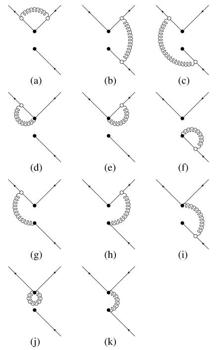
FIG. 1.: One-loop vertex corrections for the baryon number violating operator on the lattice. Solid circle denotes the vertex. Open circle is for the quark-gluon interaction either in eq.(27) or in eq.(28).

TABLE I.: Finite parts $v_{\rm diag}$ and $v_{\rm mix}$ for vertex correction of the baryon number violating operators. Coefficients of the term ${c_{\rm SW}}^{n}$ $(n=0,1,2)$ are given in the column marked as $(n)$.

gauge action		$v_{\rm diag}$			$v_{\rm mix}$
$c_{1}$	$c_{2}+c_{3}$	$(0)$	$(1)$	$(2)$	$(0)$	$(1)$	$(2)$
$0$	$0$	$11.084$	$3.3282$	$1.1498$	$-3.2137$	$3.3282$	$-1.1386$
$-1/12$	$0$	$10.743$	$2.9496$	$0.95371$	$-2.7085$	$2.9496$	$-1.0372$
$-0.331$	$0$	$10.052$	$2.3000$	$0.65335$	$-1.9381$	$2.3000$	$-0.84886$
$-0.27$	$-0.04$	$10.140$	$2.3654$	$0.67777$	$-2.0107$	$2.3654$	$-0.86909$
$-0.252$	$-0.17$	$10.020$	$2.2432$	$0.61679$	$-1.8783$	$2.2432$	$-0.83258$

TABLE II.: Finite parts $v_{\rm diag}^{\prime}$ and $v_{\rm mix}^{\prime}$ for vertex correction of the baryon number violating operators. Coefficients of the term ${c_{\rm SW}}^{n}$ $(n=0,1,2)$ are given in the column marked as $(n)$.

gauge action		$v_{\rm diag}^{\prime}$			$v_{\rm mix}^{\prime}$
$c_{1}$	$c_{2}+c_{3}$	$(0)$	$(1)$	$(2)$	$(0)$	$(1)$	$(2)$
$0$	$0$	$-25.821$	$13.753$	$-1.1792$	$-6.3894$	$4.5991$	$-1.1792$
$-1/12$	$0$	$-21.129$	$11.779$	$-1.0080$	$-5.0767$	$3.8148$	$-1.0080$
$-0.331$	$0$	$-14.319$	$8.6222$	$-0.72746$	$-3.2392$	$2.6134$	$-0.72746$
$-0.27$	$-0.04$	$-14.873$	$8.8984$	$-0.75215$	$-3.3803$	$2.7111$	$-0.75215$
$-0.252$	$-0.17$	$-13.583$	$8.2648$	$-0.69439$	$-3.0321$	$2.4672$	$-0.69439$

TABLE III.: Finite parts $v_{\rm diag}^{\prime\prime}$ and $v_{\rm mix}^{\prime\prime}$ for vertex correction of the baryon number violating operators. Coefficients of the term ${c_{\rm SW}}^{n}$ $(n=0,1,2)$ are given in the column marked as $(n)$.

gauge action		$v_{\rm diag}^{\prime\prime}$			$v_{\rm mix}^{\prime\prime}$
$c_{1}$	$c_{2}+c_{3}$	$(0)$	$(1)$	$(2)$	$(0)$	$(1)$	$(2)$
$0$	$0$	$-1.3783$	$1.1792$	$-0.35763$	$4.5459$	$-2.6297$	$0.54935$
$-1/12$	$0$	$-1.1210$	$1.0080$	$-0.31313$	$3.5094$	$-2.0995$	$0.44985$
$-0.331$	$0$	$-0.74755$	$0.72746$	$-0.23554$	$2.1314$	$-1.3427$	$0.30008$
$-0.27$	$-0.04$	$-0.77933$	$0.75215$	$-0.24280$	$2.2182$	$-1.3932$	$0.31101$
$-0.252$	$-0.17$	$-0.71136$	$0.69439$	$-0.22656$	$1.9313$	$-1.2279$	$0.27829$