DESY 99-193 ISSN 0418-9833
December 1999

Investigation of Power Corrections to
Event Shape Variables measured
in Deep-Inelastic Scattering

H1 Collaboration

Deep-inelastic $ep$ scattering data, taken with the H1 detector at HERA, are used to study the event shape variables thrust, jet broadening, jet mass, $C$ parameter and two kinds of differential two-jet rate. The data cover a large range of the four-momentum transfer $Q$, which is considered to be the relevant energy scale, between $7\,{\rm GeV}$ and $100\,{\rm GeV}$. The $Q$ dependences of the mean values are compared with second order calculations of perturbative QCD applying power law corrections proportional to $1/Q^{p}$ to account for hadronization effects. The concept of power corrections is investigated by fitting simultaneously a non-perturbative parameter $\overline{\alpha}_{p-1}$ and the strong coupling constant $\alpha_{s}$.

To be submitted to Eur. Phys. J. C

C. Adloff³³, V. Andreev²⁴, B. Andrieu²⁷, V. Arkadov³⁵, A. Astvatsatourov³⁵, I. Ayyaz²⁸, A. Babaev²³, J. Bähr³⁵, P. Baranov²⁴, E. Barrelet²⁸, W. Bartel¹⁰, U. Bassler²⁸, P. Bate²¹, O. Behnke¹⁰, C. Beier¹⁴, A. Belousov²⁴, T. Benisch¹⁰, Ch. Berger¹, G. Bernardi²⁸, T. Berndt¹⁴, G. Bertrand-Coremans⁴, P. Biddulph²¹, J.C. Bizot²⁶, K. Borras⁷, V. Boudry²⁷, W. Braunschweig¹, V. Brisson²⁶, H.-B. Bröker², D.P. Brown²¹, W. Brückner¹², P. Bruel²⁷, D. Bruncko¹⁶, J. Bürger¹⁰, F.W. Büsser¹¹, A. Bunyatyan^12,34, S. Burke¹⁷, H. Burkhardt¹⁴, A. Burrage¹⁸, G. Buschhorn²⁵, A.J. Campbell¹⁰, J. Cao²⁶, T. Carli²⁵, E. Chabert²², M. Charlet⁴, D. Clarke⁵, B. Clerbaux⁴, C. Collard⁴, J.G. Contreras^7,41, J.A. Coughlan⁵, M.-C. Cousinou²², B.E. Cox²¹, G. Cozzika⁹, J. Cvach²⁹, J.B. Dainton¹⁸, W.D. Dau¹⁵, K. Daum^33,39, M. David^9,† M. Davidsson²⁰, B. Delcourt²⁶, A. De Roeck¹⁰, E.A. De Wolf⁴, C. Diaconu²², P. Dixon¹⁹, V. Dodonov¹², K.T. Donovan¹⁹, J.D. Dowell³, A. Droutskoi²³, C. Duprel², J. Ebert³³, G. Eckerlin¹⁰, D. Eckstein³⁵, V. Efremenko²³, S. Egli³⁷, R. Eichler³⁶, F. Eisele¹³, E. Eisenhandler¹⁹, M. Ellerbrock¹³, E. Elsen¹⁰, M. Erdmann^10,40,f, A.B. Fahr¹¹, P.J.W. Faulkner³, L. Favart⁴, A. Fedotov²³, R. Felst¹⁰, J. Feltesse⁹, J. Ferencei¹⁰, F. Ferrarotto³¹, S. Ferron²⁷, M. Fleischer¹⁰, G. Flügge², A. Fomenko²⁴, I. Foresti³⁷, J. Formánek³⁰, J.M. Foster²¹, G. Franke¹⁰, E. Gabathuler¹⁸, K. Gabathuler³², J. Garvey³, J. Gassner³², J. Gayler¹⁰, R. Gerhards¹⁰, A. Glazov³⁵, L. Goerlich⁶, N. Gogitidze²⁴, M. Goldberg²⁸, I. Gorelov²³, C. Grab³⁶, H. Grässler², T. Greenshaw¹⁸, R.K. Griffiths¹⁹, G. Grindhammer²⁵, T. Hadig¹, D. Haidt¹⁰, L. Hajduk⁶, V. Haustein³³, W.J. Haynes⁵, B. Heinemann¹⁰, G. Heinzelmann¹¹, R.C.W. Henderson¹⁷, S. Hengstmann³⁷, H. Henschel³⁵, R. Heremans⁴, G. Herrera^7,41,l, I. Herynek²⁹, M. Hilgers³⁶, K.H. Hiller³⁵, C.D. Hilton²¹, J. Hladký²⁹, P. Höting², D. Hoffmann¹⁰, R. Horisberger³², S. Hurling¹⁰, M. Ibbotson²¹, Ç. İşsever⁷, M. Jacquet²⁶, M. Jaffre²⁶, L. Janauschek²⁵, D.M. Jansen¹², X. Janssen⁴, L. Jönsson²⁰, D.P. Johnson⁴, M. Jones¹⁸, H. Jung²⁰, H.K. Kästli³⁶, D. Kant¹⁹, M. Kapichine⁸, M. Karlsson²⁰, O. Karschnick¹¹, O. Kaufmann¹³, M. Kausch¹⁰, F. Keil¹⁴, N. Keller¹³, I.R. Kenyon³, S. Kermiche²², C. Kiesling²⁵, M. Klein³⁵, C. Kleinwort¹⁰, G. Knies¹⁰, H. Kolanoski³⁸, S.D. Kolya²¹, V. Korbel¹⁰, P. Kostka³⁵, S.K. Kotelnikov²⁴, M.W. Krasny²⁸, H. Krehbiel¹⁰, J. Kroseberg³⁷, D. Krücker³⁸, K. Krüger¹⁰, A. Küpper³³, T. Kuhr¹¹, T. Kurča³⁵, W. Lachnit¹⁰, R. Lahmann¹⁰, D. Lamb³, M.P.J. Landon¹⁹, W. Lange³⁵, A. Lebedev²⁴, F. Lehner¹⁰, V. Lemaitre¹⁰, R. Lemrani¹⁰, V. Lendermann⁷, S. Levonian¹⁰, M. Lindstroem²⁰, G. Lobo²⁶, E. Lobodzinska¹⁰, V. Lubimov²³, S. Lüders³⁶, D. Lüke^7,10, L. Lytkin¹², N. Magnussen³³, H. Mahlke-Krüger¹⁰, N. Malden²¹, E. Malinovski²⁴, I. Malinovski²⁴, R. Maraček²⁵, P. Marage⁴, J. Marks¹³, R. Marshall²¹, H.-U. Martyn¹, J. Martyniak⁶, S.J. Maxfield¹⁸, T.R. McMahon¹⁸, A. Mehta⁵, K. Meier¹⁴, P. Merkel¹⁰, F. Metlica¹², A. Meyer¹⁰, H. Meyer³³, J. Meyer¹⁰, P.-O. Meyer², S. Mikocki⁶, D. Milstead¹⁸, R. Mohr²⁵, S. Mohrdieck¹¹, M.N. Mondragon⁷, F. Moreau²⁷, A. Morozov⁸, J.V. Morris⁵, D. Müller³⁷, K. Müller¹³, P. Murín^16,42, V. Nagovizin²³, B. Naroska¹¹, J. Naumann⁷, Th. Naumann³⁵, I. Négri²², P.R. Newman³, H.K. Nguyen²⁸, T.C. Nicholls⁵, F. Niebergall¹¹, C. Niebuhr¹⁰, O. Nix¹⁴, G. Nowak⁶, T. Nunnemann¹², J.E. Olsson¹⁰, D. Ozerov²³, V. Panassik⁸, C. Pascaud²⁶, S. Passaggio³⁶, G.D. Patel¹⁸, E. Perez⁹, J.P. Phillips¹⁸, D. Pitzl³⁶, R. Pöschl⁷, I. Potashnikova¹², B. Povh¹², K. Rabbertz¹, G. Rädel⁹, J. Rauschenberger¹¹, P. Reimer²⁹, B. Reisert²⁵, D. Reyna¹⁰, S. Riess¹¹, E. Rizvi³, P. Robmann³⁷, R. Roosen⁴, A. Rostovtsev^23,10, C. Royon⁹, S. Rusakov²⁴, K. Rybicki⁶, D.P.C. Sankey⁵, J. Scheins¹, F.-P. Schilling¹³, S. Schleif¹⁴, P. Schleper¹³, D. Schmidt³³, D. Schmidt¹⁰, L. Schoeffel⁹, T. Schörner²⁵, A. Schoning³⁶, V. Schröder¹⁰, H.-C. Schultz-Coulon¹⁰, F. Sefkow³⁷, V. Shekelyan²⁵, I. Sheviakov²⁴, L.N. Shtarkov²⁴, G. Siegmon¹⁵, P. Sievers¹³, Y. Sirois²⁷, T. Sloan¹⁷, P. Smirnov²⁴, M. Smith¹⁸, V. Solochenko²³, Y. Soloviev²⁴, V. Spaskov⁸, A. Specka²⁷, H. Spitzer¹¹, R. Stamen⁷, J. Steinhart¹¹, B. Stella³¹, A. Stellberger¹⁴, J. Stiewe¹⁴, U. Straumann¹³, W. Struczinski², J.P. Sutton³, M. Swart¹⁴, M. Taševský²⁹, V. Tchernyshov²³, S. Tchetchelnitski²³, G. Thompson¹⁹, P.D. Thompson³, N. Tobien¹⁰, D. Traynor¹⁹, P. Truöl³⁷, G. Tsipolitis³⁶, J. Turnau⁶, J.E. Turney¹⁹, E. Tzamariudaki²⁵, S. Udluft²⁵, A. Usik²⁴, S. Valkár³⁰, A. Valkárová³⁰, C. Vallée²², P. Van Mechelen⁴, Y. Vazdik²⁴, G. Villet⁹, S. von Dombrowski³⁷, K. Wacker⁷, R. Wallny¹³, T. Walter³⁷, B. Waugh²¹, G. Weber¹¹, M. Weber¹⁴, D. Wegener⁷, A. Wegner¹¹, T. Wengler¹³, M. Werner¹³, L.R. West³, G. White¹⁷, S. Wiesand³³, T. Wilksen¹⁰, M. Winde³⁵, G.-G. Winter¹⁰, Ch. Wissing⁷, M. Wobisch², H. Wollatz¹⁰, E. Wünsch¹⁰, J. Žáček³⁰, J. Zálešák³⁰, Z. Zhang²⁶, A. Zhokin²³, P. Zini²⁸, F. Zomer²⁶, J. Zsembery⁹ and M. zur Nedden¹⁰

¹ I. Physikalisches Institut der RWTH, Aachen, Germany^a
2 III. Physikalisches Institut der RWTH, Aachen, Germany^a
3 School of Physics and Space Research, University of Birmingham, Birmingham, UK^b
4 Inter-University Institute for High Energies ULB-VUB, Brussels; Universitaire Instelling Antwerpen, Wilrijk; Belgium^c
5 Rutherford Appleton Laboratory, Chilton, Didcot, UK^b
6 Institute for Nuclear Physics, Cracow, Poland^d
7 Institut für Physik, Universität Dortmund, Dortmund, Germany^a
8 Joint Institute for Nuclear Research, Dubna, Russia
⁹ DSM/DAPNIA, CEA/Saclay, Gif-sur-Yvette, France
¹⁰ DESY, Hamburg, Germany^a
11 II. Institut für Experimentalphysik, Universität Hamburg, Hamburg, Germany^a
12 Max-Planck-Institut für Kernphysik, Heidelberg, Germany^a
13 Physikalisches Institut, Universität Heidelberg, Heidelberg, Germany^a
14 Institut für Hochenergiephysik, Universität Heidelberg, Heidelberg, Germany^a
15 Institut für experimentelle und angewandte Physik, Universität Kiel, Kiel, Germany^a
16 Institute of Experimental Physics, Slovak Academy of Sciences, Košice, Slovak Republic^f,j
17 School of Physics and Chemistry, University of Lancaster, Lancaster, UK^b
18 Department of Physics, University of Liverpool, Liverpool, UK^b
19 Queen Mary and Westfield College, London, UK^b
20 Physics Department, University of Lund, Lund, Sweden^g
21 Department of Physics and Astronomy, University of Manchester, Manchester, UK^b
22 CPPM, Université d’Aix-Marseille II, IN2P3-CNRS, Marseille, France
²³ Institute for Theoretical and Experimental Physics, Moscow, Russia
²⁴ Lebedev Physical Institute, Moscow, Russia^f,k
25 Max-Planck-Institut für Physik, München, Germany^a
26 LAL, Université de Paris-Sud, IN2P3-CNRS, Orsay, France
²⁷ LPNHE, École Polytechnique, IN2P3-CNRS, Palaiseau, France
²⁸ LPNHE, Universités Paris VI and VII, IN2P3-CNRS, Paris, France
²⁹ Institute of Physics, Academy of Sciences of the Czech Republic, Praha, Czech Republic^f,h
30 Nuclear Center, Charles University, Praha, Czech Republic^f,h
31 INFN Roma 1 and Dipartimento di Fisica, Università Roma 3, Roma, Italy
³² Paul Scherrer Institut, Villigen, Switzerland
³³ Fachbereich Physik, Bergische Universität Gesamthochschule Wuppertal, Wuppertal, Germany^a
34 Yerevan Physics Institute, Yerevan, Armenia
³⁵ DESY, Zeuthen, Germany^a
36 Institut für Teilchenphysik, ETH, Zürich, Switzerland^i
37 Physik-Institut der Universität Zürich, Zürich, Switzerlandⁱ

³⁸ Present address: Institut für Physik, Humboldt-Universität, Berlin, Germany^a
39 Also at Rechenzentrum, Bergische Universität Gesamthochschule Wuppertal, Wuppertal, Germany^a
40 Also at Institut für Experimentelle Kernphysik, Universität Karlsruhe, Karlsruhe, Germany
⁴¹ Also at Dept. Fis. Ap. CINVESTAV, Mérida, Yucatán, México
⁴² Also at University of P.J. Šafárik, SK-04154 Košice, Slovak Republic

^† Deceased

^a Supported by the Bundesministerium für Bildung, Wissenschaft, Forschung und Technologie, FRG, under contract numbers 7AC17P, 7AC47P, 7DO55P, 7HH17I, 7HH27P, 7HD17P, 7HD27P, 7KI17I, 6MP17I and 7WT87P
^b Supported by the UK Particle Physics and Astronomy Research Council, and formerly by the UK Science and Engineering Research Council
^c Supported by FNRS-FWO, IISN-IIKW
^d Partially supported by the Polish State Committee for Scientific Research, grant no. 115/E-343/SPUB/P03/002/97 and grant no. 2P03B 055 13
^e Supported in part by US DOE grant DE F603 91ER40674
^f Supported by the Deutsche Forschungsgemeinschaft
^g Supported by the Swedish Natural Science Research Council
^h Supported by GA ČR grant no. 202/96/0214, GA AV ČR grant no. A1010821 and GA UK grant no. 177
ⁱ Supported by the Swiss National Science Foundation
^j Supported by VEGA SR grant no. 2/5167/98
^k Supported by Russian Foundation for Basic Research grant no. 96-02-00019
^l Supported by the Alexander von Humboldt Foundation

1 Introduction

Hadronic final states in deep-inelastic $ep$ scattering (DIS) $ep\rightarrow eX$ offer an interesting environment to study non-perturbative hadronization phenomena and predictions of perturbative QCD over a wide range of momentum transfer $Q$ in a single experiment. A major limitation comes from the treatment of the hadronization of partons, usually modelled by phenomenological event generators. Recent theoretical developments suggest that these non-perturbative hadronization contributions may be described by ${\cal O}(1/Q^{p})$ power law corrections [1, 2] with perturbatively calculable coefficients relating their relative magnitudes. Fragmentation models are not needed.

First results on an analysis of mean event shape variables as a function of $Q$ in terms of power corrections and the strong coupling constant $\alpha_{s}(M_{Z})$ have been published by the H1 collaboration [3]. It could be shown that power corrections can be successfully applied to the variables thrust and jet mass, but they failed to describe the observed jet broadening. In order to further test the concept of power corrections, the previous work is considerably extended in the present paper. The analyzed integrated luminosity at high $Q$ is tripled, the data correction methods are refined and additional event shape variables are investigated. Theoretical progress has come from calculations of two-loop effects and the problem of jet broadening has been revisited. A comprehensive study of power corrections to the mean values of the event shape variables thrust, jet broadening, jet mass, $C$ parameter and differential two-jet rates will be presented. The data cover a large kinematical phase space of $7\,{\rm GeV}<Q<100\,{\rm GeV}$ in momentum transfer and $0.05<y<0.8$ in the inelasticity $y$.

2 Event Shapes

2.1 The Breit Frame

Event shape analyses in deep-inelastic scattering are based on the observation of the hard scattering of a quark or gluon which has to be isolated from the target (proton remnant) fragmentation region. A particularly suitable frame of reference to study the current region with minimal contamination from target fragmentation effects is the Breit frame. Consider, for illustration, $ep$ scattering in the quark parton model. In the Breit system the purely space-like gauge boson $\gamma/Z$ with four-momentum $q=\{0,0,0,-Q\}$ collides with the incoming quark with longitudinal momentum $p^{\rm in}_{q\,z}=Q/2$. The outgoing quark is back-scattered with longitudinal momentum $p^{\rm out}_{q\,z}=-Q/2$ while the proton fragments in the opposite hemisphere carrying longitudinal momentum $p_{r\,z}=Q/2\cdot(1-x)/x$, where $x$ is the fractional momentum of the struck quark in the proton with momentum $P$. Employing the boson direction as a ‘natural’ axis, the boost into the Breit frame, defined by $2x{\bf P}+{\bf q}={\bf 0}$, thus provides a clean separation into a current and a target hemisphere and may be used to classify event topologies at a scale $Q$. Higher order processes like QCD Compton scattering and boson gluon fusion modify this simple picture. However, without knowledge of the detailed structure of the hadronic final state, e.g. jet directions, the proton remnant is maximally separated from the current fragmentation.

The kinematic quantities needed to perform the Breit frame transformation are calculated from the scattered lepton ($E_{e^{\prime}},\theta_{e^{\prime}}$) and hadron measurements ($E_{i},\theta_{i}$) where $i$ runs over all hadronic objects:

$$Q^{2} = 4E_{e}E_{e^{\prime}}\cos^{2}\frac{\theta_{e^{\prime}}}{2}\,,$$ (1)

$$y\equiv y_{e} = 1-\frac{E_{e^{\prime}}}{E_{e}}\sin^{2}\frac{\theta_{e^{\prime}}}{2}\quad\quad\quad\quad{\rm for}\quad y_{e}>0.15\,,$$ (2)

$$y\equiv y_{h} = \frac{\sum\limits_{i}E_{i}(1-\cos\theta_{i})}{2E_{e}}\quad\quad\quad\,\,{\rm for}\quad y_{e}<0.15\,,$$ (3)

with $E_{e}=27.5\,{\rm GeV}$ and $E_{p}=820\,{\rm GeV}$ being the beam energies. The inelasticity $y=y_{e}$ is chosen for sufficiently large values. However, since the resolution in $y_{e}$ degrades severely at low values, $y=y_{h}$ is taken if $y_{e}<0.15$. This procedure ensures least uncertainty in the Lorentz transformation to the Breit frame.

2.2 Definition of Event Shape Variables

The dimensionless event shape variables thrust, jet broadening, $C$ parameter and jet mass are studied in the current hemisphere (CH) of the Breit system. The sums extend over all particles $h$ of the hadronic final state in the CH with four-momenta $p_{h}=\{E_{h},{\bf p}_{h}\}$. The current hemisphere axis ${\bf n}=\{0,0,-1\}$ coincides with the boson direction. The following collinear- and infrared-safe definitions of event shape variables are used:

Thrust $\tau\equiv 1-T$ measures the longitudinal momentum components projected onto the current hemisphere axis

$$\tau = 1-\frac{\sum\limits_{\scriptscriptstyle h\in{\rm CH}}|{\bf p}_{h}\cdot{\bf n}|}{\sum\limits_{\scriptscriptstyle h\in{\rm CH}}|{\bf p}_{h}|}\ =\ 1-\frac{\sum\limits_{\scriptscriptstyle h\in{\rm CH}}|{\bf p}_{z\,h}|}{\sum\limits_{\scriptscriptstyle h\in{\rm CH}}|{\bf p}_{h}|}\,.$$ (4)

Thrust $\tau_{C}\equiv 1-T_{C}$ uses the direction ${\bf n}_{T}$ which maximizes the sum of the longitudinal momenta of all particles in the current hemisphere along this axis

$$\tau_{C} = 1-\max_{\scriptscriptstyle{\bf n^{\prime}},{\bf n^{\prime}}^{2}=1}\frac{\sum\limits_{\scriptscriptstyle h\in{\rm CH}}|{\bf p}_{h}\cdot{\bf n^{\prime}}|}{\sum\limits_{\scriptscriptstyle h\in{\rm CH}}|{\bf p}_{h}|}=1-\frac{\sum\limits_{\scriptscriptstyle h\in{\rm CH}}|{\bf p}_{h}\cdot{\bf n}_{T}|}{\sum\limits_{\scriptscriptstyle h\in{\rm CH}}|{\bf p}_{h}|}\,.$$ (5)

This definition is analogous to that used in $e^{+}e^{-}$  experiments and represents a mixture of longitudinal and transverse momenta with respect to the boson axis.

The Jet Broadening $B$ measures the scalar sum of transverse momenta with respect to the current hemisphere axis

$$B = \frac{\sum\limits_{\scriptscriptstyle h\in{\rm CH}}|{\bf p}_{h}\times{\bf n}|}{2\,\sum\limits_{\scriptscriptstyle h\in{\rm CH}}|{\bf p}_{h}|}\ =\ \frac{\sum\limits_{\scriptscriptstyle h\in{\rm CH}}|{\bf p}_{\perp\,h}|}{2\,\sum\limits_{\scriptscriptstyle h\in{\rm CH}}|{\bf p}_{h}|}\,.$$ (6)

The squared Jet Mass $\rho$ is normalized to four times the squared total energy in the current hemisphere

$$\rho = \frac{(\sum\limits_{\scriptscriptstyle h\in{\rm CH}}p_{h})^{2}}{(2\,\sum\limits_{\scriptscriptstyle h\in{\rm CH}}E_{h})^{2}}\,.$$ (7)

The $C$ Parameter is derived from the eigenvalues $\lambda_{i}$ of the linearized momentum tensor $\Theta^{jk}$

$$\Theta^{jk} = \frac{\sum\limits_{\scriptscriptstyle h\in{\rm CH}}p^{j}_{h}p^{k}_{h}/|{\bf p}_{h}|}{\sum\limits_{\scriptscriptstyle h\in{\rm CH}}|{\bf p}_{h}|}$$

$$C = 3(\lambda_{1}\lambda_{2}+\lambda_{2}\lambda_{3}+\lambda_{3}\lambda_{1})\,.$$ (8)

The real symmetric matrix $\Theta^{jk}$ has eigenvalues $\lambda_{i}$ with $0<\lambda_{3}\leq\lambda_{2}\leq\lambda_{1}<1$. It describes an ellipsoid with orthogonal axes named minor, semi-major and major corresponding to the three eigenvalues. The major axis is similar but not identical to ${\bf n}_{T}$. If all momenta are collinear then two eigenvalues and hence $C$ are equal to zero.

Higher order processes may lead to event configurations where the partons are scattered into the target hemisphere and the current hemisphere may be completely empty except for migrations due to hadronization fragments. In order to be insensitive to such effects and to keep the event shape variables infrared safe [4] the total available energy in the current hemisphere has to exceed $20\%$ of the value expected in the quark parton model

$$E_{CH}\equiv\sum\limits_{\scriptscriptstyle h\in{\rm CH}}E_{h} > Q/10\,.$$ (9)

Otherwise the event is ignored. This cut-off is part of the event shape definitions, its precise value is not critical.

The event shapes defined in the current hemisphere may be distinguished according to the event axis used. Thrust $\tau$ and the jet broadening $B$ employ momentum vectors projected onto the boson direction. Thrust $\tau_{C}$ and the $C$ parameter calculate their own axis, while the jet mass $\rho$ does not depend on any event orientation.

Another class of event shapes investigates the number of $(n+1)$ jets found in an event, where $+1$ denotes the proton remnant. Jets are searched for in the complete accessible phase space, i.e. in both the current and target hemispheres of the Breit frame. Two schemes of jet definitions are applied: the Durham or $k_{t}$ algorithm [5] and a factorizable Jade algorithm [6] adapted to DIS. Both jet finding procedures introduce two distance measures: one for distances between two four-vectors, $y_{ij}$, and another one for the separation of each particle from the remnant, $y_{ir}$. The following distance measures are used:

Durham or $$k_{t}$$ algorithm

$$y_{ij} = \frac{2\min(E_{i}^{2},E_{j}^{2})(1-\cos\theta_{ij})}{Q^{2}}\,,$$ (10)

$$y_{ir} = \frac{2E_{i}^{2}(1-\cos\theta_{ir})}{Q^{2}}\,,$$ (11)

factorizable Jade algorithm

$$y_{ij} = \frac{2E_{i}E_{j}(1-\cos\theta_{ij})}{Q^{2}}\,,$$ (12)

$$y_{ir} = \frac{2E_{i}xE_{p}(1-\cos\theta_{ir})}{Q^{2}}\,,$$ (13)

where $\theta_{kl}$ is the angle between the two momentum vectors. Since the direction of the proton remnant coincides with the $+z$ axis for the coordinate system chosen here $\theta_{ir}$ simplifies to the polar angle $\theta_{i}$. The pair with the minimal $y_{ij}$ or $y_{ir}$ value of all possible combinations is selected to either form a new pseudo-particle vector or to assign the particle $i$ to the remnant. The whole procedure is repeated until a certain number of jets is found. The event shape variables $y_{k_{t}}$ ($k_{t}$ algorithm) and $y_{fJ}$ (factorizable Jade algorithm) are defined as that $y$ value $y_{ij}$ or $y_{ir}$ where the transition from $(2+1)\rightarrow(1+1)$ jets occurs.

Throughout the paper the symbol $F$ will be used as a generic name for any event shape variable defined above. Note that for all of them $F\rightarrow 0$ in case of quark parton model like reactions. Theoretical calculations of event shape distributions and means will be discussed in section 5.

3 H1 Detector and Event Selection

3.1 The H1 Detector

Deep-inelastic $ep$ scattering events were collected during the years $1994-1997$ with the H1 detector [7] at HERA. Electrons or positrons with $E_{e}=27.5\,{\rm GeV}$ collide with $E_{p}=820\,{\rm GeV}$ protons at a center of mass energy of $\sqrt{s}=300\,{\rm GeV}$. Only calorimetric information is used to reconstruct the final state. The direction of the scattered lepton and the event vertex are obtained by exploiting additional information from the tracking detectors. The calorimeters cover the polar angles $4{{}^{\circ}}\leq\theta\leq 176{{}^{\circ}}$ and the full azimuth.

The calorimeter system consists of a liquid argon (LAr) calorimeter, a backward calorimeter and a tail catcher (instrumented iron yoke). The LAr sampling calorimeter ($4{{}^{\circ}}\leq\theta\leq 154{{}^{\circ}}$) consists of a lead/argon electromagnetic section and a stainless steel/argon section for the measurement of hadronic energy. A detailed in situ calibration provides the accurate energy scales. The lepton energy uncertainty in the LAr calorimeter varies between $1\%$ in the backward region and $3\%$ in the forward region. The systematic uncertainty of the hadronic energy amounts to $4\%$. A lead/scintillator electromagnetic backward calorimeter (BEMC) extends the coverage at large angles ($155{{}^{\circ}}\leq\theta\leq 176{{}^{\circ}}$) and is used to measure the lepton at $Q\leq 10\,{\rm GeV}$ with a precision of $1\%$ for the absolute calibration. Since $1995$ the backward region has been equipped with a lead/scintillating fibre calorimeter improving the uncertainty in the measurement of hadronic energies in the backward region from $15\%$ to $7\%$. The instrumented iron flux return yoke is used to measure the leakage of hadronic showers.

Located inside the calorimeters is a tracking system which consists of central drift and proportional chambers ($25{{}^{\circ}}\leq\theta\leq 155{{}^{\circ}}$), a forward track detector ($7{{}^{\circ}}\leq\theta\leq 25{{}^{\circ}}$) and a backward proportional chamber ($155{{}^{\circ}}\leq\theta\leq 175{{}^{\circ}}$). In $1995$ the latter was replaced by backward drift chambers. The direction of the scattered lepton is determined by associating tracking information with the corresponding electromagnetic cluster. The lepton scattering angle is known to within $3\,{\rm mrad}$. The tracking chambers and calorimeters are surrounded by a superconducting solenoid providing a uniform field of $1.15\,{\rm T}$ inside the tracking volume.

3.2 Event Selection

The DIS data are divided into a low $Q$ event sample ($Q=7-10\,{\rm GeV}$, lepton detected in BEMC) and a high $Q$ event sample ($Q=14-100\,{\rm GeV}$, lepton detected in LAr calorimeter) which in turn are subdivided further into eight bins in $Q$: $7-8\,{\rm GeV}$, $8-10\,{\rm GeV}$, $14-16\,{\rm GeV}$, $16-20\,{\rm GeV}$, $20-30\,{\rm GeV}$, $30-50\,{\rm GeV}$, $50-70\,{\rm GeV}$ and $70-100\,{\rm GeV}$. The following event selection criteria ensure a good measurement of the final state and a clean data sample:

1. The energy of the isolated scattered lepton has to exceed $E_{e^{\prime}}>14\,{\rm GeV}$ within $157{{}^{\circ}}<\theta_{e^{\prime}}<173{{}^{\circ}}$ for the low $Q$ sample and $E_{e^{\prime}}>11\,{\rm GeV}$ within $30{{}^{\circ}}<\theta_{e^{\prime}}<150{{}^{\circ}}$ for the high $Q$ sample respectively. The calorimetric lepton trigger efficiencies are above $99\%$ [7, 8].

2. The inelasticity $y$ is well measured by requiring $0.05<y_{e}<0.8$ (using the lepton) and $0.05<y_{h}$ (using the hadronic energy flow). This criterion suppresses photoproduction events with a misidentified lepton.

3. The ‘quark’ direction as calculated from the scattered lepton in the quark parton model corresponds to the $-z$ axis of the Breit frame. A minimal value of $\theta_{q}>20{{}^{\circ}}$ in the laboratory system ensures a sufficient detector resolution in polar angle after transformation into the Breit frame.

4. A minimal energy in the Breit current hemisphere of $Q/10$ (see eq. (9) of section 2.2) is essential to keep the event shapes $\tau$, $B$, $\tau_{C}$, $\rho$ and $C$ infrared safe. This is part of their definition.

5. To avoid unphysical peaks at zero for $\tau_{C}$, $\rho$ and $C$ at least two hadronic objects are required. Events containing only one such object are not quark parton model like but are due to leakage into the current hemisphere.

6. The total energy in the forward region $(4{{}^{\circ}}<\theta<15{{}^{\circ}})$ has to be larger than $0.5\,{\rm GeV}$ to reduce the proportion of diffractive events which are not included into the theoretical description of the data.

7. Hadron clusters have to be contained in the calorimeter acceptance of $5.7{{}^{\circ}}<\theta_{h}<170{{}^{\circ}}$ avoiding the edges close to the beam pipe. The hadronic energy measured in the backward region $\theta_{h}\geq 170{{}^{\circ}}$ has to be less than $10\,{\rm GeV}$ in order to exclude poor measurements.

8. The total longitudinal energy balance must satisfy $30\,{\rm GeV}<\sum_{i}E_{i}(1-\cos\theta_{i})<65\,{\rm GeV}$ in order to suppress initial state photon radiation and to further reduce photoproduction background.

9. The total transverse momentum has to be $|\vec{p}_{\perp}|<7.5\,{\rm GeV}$ (low $Q$ sample) and $|\vec{p}_{\perp}|<15\,{\rm GeV}$ (high $Q$ sample), respectively, in order to exclude badly measured events.

10. The energy measurement of the lepton has to be consistent with that derived from the double angle method [9] $|(E_{e^{\prime}}-E_{da})/E_{da}|<0.25$ in order to further suppress events strongly affected by QED radiation. $E_{da}$ is calculated from the directions of the lepton and the hadronic energy flow.

11. An event vertex has to exist within $3\sigma$ of the nominal $z$ position of the interaction point $|z_{v}-\langle z_{v}\rangle|<35\,{\rm cm}$.

12. Leptons pointing to dead regions of the LAr calorimeter, i.e. $\pm 2{{}^{\circ}}$ around $\phi$-cracks between modules or $\pm 5\,{\rm cm}$ around $z$-cracks between wheels, are rejected in order to ensure a reliable measurement.

The event selection criteria can be separated into phase space cuts, nos. $1-4$, representing the common requirements for data and theory, and data quality cuts, nos. $5-12$. Note that the cuts nos. $5$ and $6$ are always applied except for the perturbative QCD calculations described in section 5 where they do not make sense. Depending on the theoretical model to compare with they may be considered as phase space cuts as well. Not all cuts affect both the low and high $Q$ data samples, as can be seen from the distribution of events in the $x-Q^{2}$ plane shown in figure 1.

The contamination from photoproduction background is estimated to be less than $3\%$ in the low $Q$ sample and negligible at higher values of $Q$. Residual radiative effects are accounted for by the data correction procedure described in section 4.

The final data samples consist of $9,761$ events at $Q=7-10\,{\rm GeV}$ taken in $1994$ with an integrated luminosity of ${\cal L}=3.2~{}\,{\rm pb}^{-1}$ and $42,607$ events at $Q=14-100\,{\rm GeV}$ corresponding to ${\cal L}=38.2~{}\,{\rm pb}^{-1}$ recorded from $1994-1997$.

Figure 1: Distribution of selected events in the $x-Q^{2}$ plane. Only a small part of the data corresponding to a luminosity of $3.2\,{\rm pb}^{-1}$ is shown. The curves indicate the phase space cuts in $E_{e^{\prime}}$, $\theta_{e^{\prime}}$, $y$ and $\theta_{q}$.

4 Measurement of Event Shapes

The aim of the analysis is to present measured event shape variables and to compare with second order calculations of perturbative QCD (pQCD) supplemented with analytical power-law corrections to account for hadronization effects. The experimental observables need to be corrected for detector effects and QED radiation. Such a procedure involves Monte Carlo event generators and hence introduces some model dependencies which are taken into account in the analysis of systematic uncertainties. They are much smaller than those obtained in approaches which try to unfold from the data to a ‘partonic final state’ which is directly comparable to pQCD.

4.1 Event Simulation

A detailed detector simulation is done by using event samples generated with the Django [10] Monte Carlo program. The modelling of parton showers involves a colour dipole model as implemented in Ariadne [11]. Alternatively, Django in combination with Lepto [12] without soft colour interactions has been used to investigate the model dependence. The hadronization of partons uses the Jetset [13] string fragmentation. QED radiation on the lepton side, including real photons and virtual 1-loop corrections, is treated by Heracles [14]. Both DIS packages provide a reasonable description of the measured event shape distributions and are used to correct the data. The event generators Lepto with soft colour interactions and Herwig [15] as stand-alone programs without QED radiation differ considerably in their predictions for the hadronic final state and serve to cross-check the unfolding methods.

4.2 Data Correction Procedure

The data analysis proceeds in two steps. First the data are corrected for detector effects within the phase space described in section 3.2 applying different techniques. In a second step QED radiation and acceptance corrections due to the beam hole (cut no. 7) are taken into account.

The most reliable method considered to correct event shape distributions for detector effects is found to be a Bayesian unfolding procedure [16]. This technique exploits Bayes’ theorem on conditional probabilities to extract information on the underlying distribution from the observed distribution. Although some a priori knowledge on the initial distribution is required — it may even be assumed to be uniform in the case of complete ignorance — the iterative procedure is very robust and converges to stable results within three steps. The program takes correlations properly into account.

Alternatively, the matrix method employed in the previous publication [3] and simple correction factors applied either bin-by-bin to the distributions or directly to the mean values have been used. They serve to estimate systematic effects. The performance of these correction techniques is checked by studying the spectra and mean values of the event shapes when unfolding one Monte Carlo with another and vice versa for various combinations of event generators. In general, the Bayes method gives the best results; for details see [17].

The remaining corrections account for QED radiation effects and beam hole losses. They are applied on a bin-by-bin basis. Non-radiative events are generated using Django with exactly the same conditions as before except for the radiative effects being switched off. A detector simulation is not required. The corrections are based on the predictions for the hadronic final state within the kinematic phase space.

The derived bin-to-bin correction factors of the event shape spectra are close to one except for $\tau$, $B$ and $y_{k_{t}}$. For $\tau$ and $B$, which are defined with respect to the boson axis, radiative effects are important and non-negligible. The differential two-jet rate $y_{k_{t}}$ is the only variable which is sensitive to acceptance losses, particularly at low $Q$. All other event shapes are almost unaffected by the beam hole cut as expected for the variables defined in the current hemisphere. Both Monte Carlo samples, i.e. Django/Ariadne and Django/Lepto, give consistent results.

4.3 Results on Event Shape Measurements

The data correction is performed with the Ariadne event generator as implemented in the Django Monte Carlo program. The final results are based on the differential distributions obtained with the Bayes unfolding and subsequent bin-to-bin radiative correction from which the mean values are calculated. The total experimental uncertainties of both the spectra and mean values are evaluated in the same way. The statistical uncertainties include data as well as Monte Carlo statistics. The systematic uncertainties are estimated by comparing the bin contents and mean of the ‘standard’ distribution with the values obtained under different conditions or assumptions. The effects of various correction procedures and the knowledge of the calorimeter energy scales are considered. Systematics from the model dependence of the Monte Carlo simulation are negligible for the event shapes defined in the current hemisphere alone. In case of the $y$ variables the results achieved with Django/Ariadne and Django/Lepto are averaged and half of the spread is taken as an estimate of the uncertainty.

Unfolding uncertainties, being in general asymmetric, are estimated to be half the maximal deviation to larger and smaller values respectively due to the alternative unfolding procedures. The sum of upper and lower deviation corresponds to half the total spread and so is somewhat smaller than twice the standard deviation of a uniform distribution. The influence of the energy scale uncertainties is taken into account by repeating the whole analysis and scaling both the electromagnetic and hadronic energies separately upwards and downwards by the appropriate amount. The discrepancies with respect to the central values are attributed to two further asymmetric systematic uncertainties. All three (four in case of $y$) error sources, i.e. the unfolding bias, the two energy scales and the model dependence, added in quadrature yield the total systematics.

For the event shapes $\tau$, $B$, $\tau_{C}$, $\rho$ and $C$, the lepton energy uncertainty, which directly affects the boost into the Breit frame, is the largest individual contribution, followed by unfolding effects. This can be understood because hadronic systematics cancel between numerator and denominator for these variables. The situation is reversed for $y_{fJ}$ and $y_{k_{t}}$. Here, no cancellation occurs and the systematic uncertainty due to hadronic energies is the larger of the two energy scale uncertainties.

The corrected event shape distributions are shown in figures 2 and 3 over a wide range of $\left<Q\right>=7.5-81.3\,{\rm GeV}$. Although the shapes of the spectra for each variable $F$ are quite different, their common feature is that they all develop to narrower distributions shifted towards lower values of $F$ as the available energy $Q$ increases. It demonstrates that the events become more collimated. A comparison with the predictions of pQCD reveals serious discrepancies especially at low $Q$ leading to the necessity to include hadronization corrections. Such corrections are discussed in the next section for the mean values of the distributions.

The measured mean values are listed in table 1. Note that the quoted uncertainties do not give the correlations due to common systematic error sources. Such correlations are, however, properly taken into account in the QCD analysis (see section 6.3).

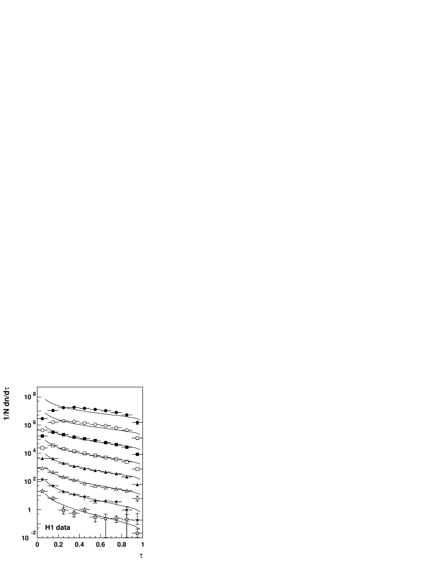
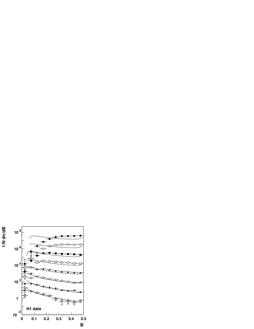
Figure 2: Normalized differential distributions of the event shapes $\tau$, $B$ and $\tau_{C}$. H1 data (symbols) are compared with Disent NLO calculations (curves) using the MRSA’ parton density functions with $\alpha_{s}(M_{Z})=0.115$. The error bars represent statistical and systematic uncertainties. The spectra given at $\left<Q\right>=7.5\,{\rm GeV},\;8.7\,{\rm GeV},\ 15.0\,{\rm GeV},\ 17.8\,{\rm GeV},\ 23.6\,{\rm GeV},\ 36.7\,{\rm GeV},\ 57.7\,{\rm GeV}$ and $81.3\,{\rm GeV}$ (from top to bottom) are multiplied by factors of $10^{n}\ (n=7,\ldots,0)$.

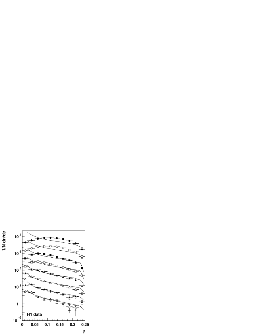
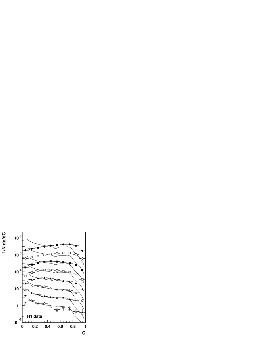
Figure 3: Normalized differential distributions of the event shapes $\rho$, $C$, $y_{fJ}$ and $y_{k_{t}}$. H1 data (symbols, see fig. 2) are compared with Disent NLO calculations (curves) using the MRSA’ parton density functions with $\alpha_{s}(M_{Z})=0.115$. The error bars represent statistical and systematic uncertainties. The spectra given at $\left<Q\right>=7.5\,{\rm GeV},\;8.7\,{\rm GeV},\ 15.0\,{\rm GeV},\ 17.8\,{\rm GeV},\ 23.6\,{\rm GeV},\ 36.7\,{\rm GeV},\ 57.7\,{\rm GeV}$ and $81.3\,{\rm GeV}$ (from top to bottom) are multiplied by factors of $10^{n}\ (n=7,\ldots,0)$.

$\rule[-8.61108pt]{0.0pt}{21.52771pt}\left<Q\right>/\,{\rm GeV}$	$\left<\tau\right>$	$\left<B\right>$
$7.5$	$0.4402\pm 0.0082~{}^{+0.0111}_{-0.0122}$	$0.3624\pm 0.0034~{}^{+0.0046}_{-0.0038}$
$8.7$	$0.4017\pm 0.0090~{}^{+0.0196}_{-0.0080}$	$0.3435\pm 0.0040~{}^{+0.0076}_{-0.0037}$
$15.0$	$0.3052\pm 0.0034~{}^{+0.0081}_{-0.0075}$	$0.2921\pm 0.0017~{}^{+0.0044}_{-0.0033}$
$17.8$	$0.2762\pm 0.0029~{}^{+0.0091}_{-0.0059}$	$0.2760\pm 0.0016~{}^{+0.0054}_{-0.0034}$
$23.6$	$0.2279\pm 0.0031~{}^{+0.0125}_{-0.0071}$	$0.2452\pm 0.0018~{}^{+0.0078}_{-0.0042}$
$36.7$	$0.1814\pm 0.0049~{}^{+0.0107}_{-0.0065}$	$0.2094\pm 0.0031~{}^{+0.0083}_{-0.0053}$
$57.9$	$0.1330\pm 0.0089~{}^{+0.0092}_{-0.0092}$	$0.1717\pm 0.0062~{}^{+0.0109}_{-0.0096}$
$81.3$	$0.0984\pm 0.0130~{}^{+0.0045}_{-0.0051}$	$0.1346\pm 0.0088~{}^{+0.0117}_{-0.0041}$

$\rule[-8.61108pt]{0.0pt}{21.52771pt}\left<Q\right>/\,{\rm GeV}$	$\left<\tau_{C}\right>$	$\left<\rho\right>$	$\left<C\right>$
$7.5$	$0.1637\pm 0.0032~{}^{+0.0030}_{-0.0029}$	$0.1115\pm 0.0019~{}^{+0.0011}_{-0.0013}$	$0.5601\pm 0.0082~{}^{+0.0083}_{-0.0073}$
$8.7$	$0.1600\pm 0.0037~{}^{+0.0060}_{-0.0031}$	$0.1044\pm 0.0021~{}^{+0.0017}_{-0.0000}$	$0.5524\pm 0.0094~{}^{+0.0074}_{-0.0054}$
$15.0$	$0.1333\pm 0.0013~{}^{+0.0013}_{-0.0019}$	$0.0872\pm 0.0007~{}^{+0.0007}_{-0.0014}$	$0.4824\pm 0.0034~{}^{+0.0036}_{-0.0051}$
$17.8$	$0.1263\pm 0.0011~{}^{+0.0014}_{-0.0024}$	$0.0826\pm 0.0007~{}^{+0.0013}_{-0.0015}$	$0.4621\pm 0.0030~{}^{+0.0045}_{-0.0069}$
$23.6$	$0.1098\pm 0.0012~{}^{+0.0020}_{-0.0026}$	$0.0714\pm 0.0007~{}^{+0.0019}_{-0.0016}$	$0.4112\pm 0.0033~{}^{+0.0056}_{-0.0076}$
$36.7$	$0.0985\pm 0.0021~{}^{+0.0012}_{-0.0023}$	$0.0634\pm 0.0012~{}^{+0.0013}_{-0.0013}$	$0.3644\pm 0.0058~{}^{+0.0029}_{-0.0058}$
$57.9$	$0.0834\pm 0.0040~{}^{+0.0015}_{-0.0046}$	$0.0518\pm 0.0023~{}^{+0.0016}_{-0.0025}$	$0.3127\pm 0.0122~{}^{+0.0065}_{-0.0131}$
$81.3$	$0.0663\pm 0.0057~{}^{+0.0031}_{-0.0025}$	$0.0410\pm 0.0034~{}^{+0.0022}_{-0.0016}$	$0.2529\pm 0.0173~{}^{+0.0160}_{-0.0065}$

$\rule[-8.61108pt]{0.0pt}{21.52771pt}\left<Q\right>/\,{\rm GeV}$	$\left<y_{fJ}\right>$	$\left<y_{k_{t}}\right>$
$7.5$	$0.1598\pm 0.0026~{}^{+0.0048}_{-0.0049}$	$0.3088\pm 0.0065~{}^{+0.0081}_{-0.0145}$
$8.7$	$0.1497\pm 0.0030~{}^{+0.0055}_{-0.0049}$	$0.2320\pm 0.0062~{}^{+0.0099}_{-0.0091}$
$15.0$	$0.1260\pm 0.0015~{}^{+0.0063}_{-0.0058}$	$0.1349\pm 0.0025~{}^{+0.0078}_{-0.0065}$
$17.8$	$0.1180\pm 0.0014~{}^{+0.0052}_{-0.0053}$	$0.1147\pm 0.0021~{}^{+0.0067}_{-0.0059}$
$23.6$	$0.1049\pm 0.0015~{}^{+0.0050}_{-0.0052}$	$0.0940\pm 0.0022~{}^{+0.0061}_{-0.0044}$
$36.7$	$0.0861\pm 0.0025~{}^{+0.0037}_{-0.0049}$	$0.0627\pm 0.0028~{}^{+0.0047}_{-0.0022}$
$57.9$	$0.0785\pm 0.0053~{}^{+0.0049}_{-0.0066}$	$0.0463\pm 0.0044~{}^{+0.0055}_{-0.0028}$
$81.3$	$0.0608\pm 0.0071~{}^{+0.0052}_{-0.0057}$	$0.0333\pm 0.0050~{}^{+0.0050}_{-0.0035}$

Table 1: Corrected mean values of the event shapes as a function of $Q$. The first uncertainty is statistical, the second systematic.

5 Theoretical Framework

Infrared and collinear safe event shape variables are presently calculable in DIS up to next-to-leading order QCD. Several programs are available. However, for comparisons to real experimental situations this is insufficient and a phenomenological description of hadronization is needed. Within the concept of power corrections one assumes that a parameterization of the leading corrections to the perturbative prediction can be obtained without modelling all the details of the hadronization. This leads to the notion of ‘universal’ power corrections with a definite $Q$ dependence, typically ${\cal O}(1/Q^{p})$, given in analytic form with a calculable coefficient for each event shape observable. The hope is that such a simplifying approach gives useful insight in the interplay of perturbative and non-perturbative effects.

5.1 pQCD Calculations

The mean value of an event shape variable $F$ can be written in second order perturbative QCD as

$$\left<F\right>^{{\rm pert}} = c_{1}(x,Q)\,\alpha_{s}(\mu_{\scriptscriptstyle R})+\left[c_{2}(x,Q)+\frac{\beta_{0}}{2\pi}\ln\frac{\mu_{\scriptscriptstyle R}}{Q}c_{1}(x,Q)\right]\alpha_{s}^{2}(\mu_{\scriptscriptstyle R})\,,$$ (14)

where $\mu_{\scriptscriptstyle R}$ is the renormalization scale, $\beta_{0}=11-2/3\,N_{f}$ and $N_{f}=5$ is the number of active flavours. In contrast to $e^{+}e^{-}$ annihilation, where the coefficients $c_{1}$ and $c_{2}$ are constant, in DIS they depend on $x$ according to the parton density functions and the accessible $x$-range at different values of $Q$ (see figure 1). Examples for a strong and a weak variation with $x$ of the mean values $\left<\tau\right>$ and $\left<C\right>$ versus $Q$ are presented in figure 4.

Figure 4: Mean values of $\tau$ (left) and $C$ (right) versus $Q$ in four different bins of $x$ calculated with Disent. The lines connect the means belonging to the same $x$ bin.

Average values of the coefficients $c_{1}$ and $c_{2}$ are calculated separately for every $Q$ bin with its specific range of $x$-values. This approximation by step functions is the origin of the steps exhibited by the curves in figures 5 and 6. The slope within one bin is due to the variation of $\alpha_{s}$ with $Q$. In the previous publication [3], average coefficients determined for the complete range in $Q$ have been employed.

The event shape means are evaluated at the scale $\mu_{\scriptscriptstyle R}=Q$ with the Disent [18] program which treats deep-inelastic $ep$ scattering to ${\cal O}(\alpha_{s}^{2})$ in the $\overline{\mbox{MS}}$ scheme and employs the subtraction method for the necessary integrations. In order to test the reliability of the perturbative predictions, careful comparisons of Mepjet [19], Disent and Disaster++ [20] have been carried out [21]. Due to intrinsic restrictions of the integration technique applied in Mepjet (phase space slicing), however, it can not be used for the mean event shapes. In general, good agreement at the percent level is observed but some discrepancies have been revealed. These are partially understood and an improved Disent version has been employed. The effects are hardly visible in the event shape spectra, but the mean values have increased considerably in the low $Q$ region compared to the calculations used in [3]. The worst case is the jet broadening $B$ whose mean value at $Q=7.5\,{\rm GeV}$ rose by about $14\%$, being still slightly different from the Disaster++ calculation.

The parton density distributions MRSA’ [22] with $\alpha_{s}(M_{Z})=0.115$ are used as standard. Other sets, i.e. MRST99 [23] and CTEQ4 [24], are investigated as well to estimate systematic uncertainties.

5.2 Power Corrections

Hadronization effects on event shapes are treated within the concept of power corrections [1, 2]. The observable mean values can be written as

$$\left<F\right> = \left<F\right>^{\rm pert}+\left<F\right>^{\rm pow}\,,$$ (15)

with $\left<F\right>^{\rm pert}$ given by eq. (14). The hadronization contributions $\left<F\right>^{\rm pow}$ are expected to be proportional to $1/Q^{p}$ with exponents $p=1$ or $p=2$ depending on the observable. Two types of parameterizations for $\left<F\right>^{\rm pow}$ will be investigated.

In a simplistic approach inspired by the longitudinal phase space or tube model, described e.g. in [25], one has

$$\left<F\right>^{\rm pow}=\frac{\lambda_{1,\,F}}{Q} {\rm or} \left<F\right>^{\rm pow}=\frac{\lambda_{2,\,F}}{Q^{2}}\,,$$ (16)

where $\lambda_{1,\,F}$ and $\lambda_{2,\,F}$ are constants. One expects $\lambda_{1}$ to be in the order of $\simeq 1\,{\rm GeV}$ and terms with exponents $p>1$ to be negligible except for the differential two-jet rate $y_{k_{t}}$. Even within this simple model it is possible to derive approximate relations between the constants $\lambda_{1}$ for different event shapes, e.g. $\lambda_{1,\,\tau}\simeq 2\,\lambda_{1,\,\rho}$, consistent with $e^{+}e^{-}$ data [25].

In the model pioneered by Dokshitzer and Webber [1, 2] the idea is to attribute $1/Q^{p}$ power-law corrections to soft gluon phenomena associated with the behaviour of the strong coupling at small scales. This leads to the notion of a universal infrared-finite effective coupling $\alpha_{\rm eff}(\mu_{\scriptscriptstyle R})$ which replaces the perturbative form in the infrared region $\mu_{\scriptscriptstyle R}<\mu_{\scriptscriptstyle I}$ where $\mu_{\scriptscriptstyle I}$, the infrared matching scale, has to fulfil $\Lambda_{\rm QCD}\ll\mu_{\scriptscriptstyle I}\approx 2\,{\rm GeV}\ll Q$. At the expense of one new non-perturbative parameter $\overline{\alpha}_{p-1}(\mu_{\scriptscriptstyle I})$, corresponding to the $(p-1)$th moment of the effective coupling $\alpha_{\rm eff}(\mu_{\scriptscriptstyle R})$ when integrated from $0$ up to $\mu_{\scriptscriptstyle I}$, the power corrections to all event shapes with the same exponent $p$ can be related via [26, 28]

$$\left<F\right>^{\rm pow} = a_{F}\,{\cal P}\,,$$ (17)

$${\cal P} = \frac{4C_{F}}{\pi\ p}{\cal M^{\prime}}\left(\frac{\mu_{\scriptscriptstyle I}}{\mu_{\scriptscriptstyle R}}\right)^{p}\left[\overline{\alpha}_{p-1}(\mu_{\scriptscriptstyle I})-\alpha_{s}(\mu_{\scriptscriptstyle R})-\frac{\beta_{0}}{2\pi}\left(\ln\frac{\mu_{\scriptscriptstyle R}}{\mu_{\scriptscriptstyle I}}+\frac{K}{\beta_{0}}+\frac{1}{p}\right)\alpha_{s}^{2}(\mu_{\scriptscriptstyle R})\right]$$ (18)

where $C_{F}=4/3$, $K=67/6-\pi^{2}/2-5/9\,N_{f}$ and $N_{f}=5$ as in the perturbative part. Again, $\mu_{\scriptscriptstyle R}$ is identified with $Q$ in this study. The subtractions proportional to $\alpha_{s}$ and $\alpha_{s}^{2}$ serve to avoid double counting.

The coefficients $a_{F}$, given in table 3, depend on the observable $F$ but can in principle be derived from a perturbative ansatz, although not yet available for the variable $y_{k_{t}}$. Some of them have changed considerably — e.g. $a_{B}$ and $a_{C}$ by factors of $4$ and $2$ respectively — from their original values [28] applied in previous investigations [3, 29]. Ambiguities in calculating the $a_{F}$ predictions could be resolved with the advent of a two-loop analysis provided an additional common coefficient, the Milan factor ${\cal M}$ [26, 27] with

$${\cal M^{\prime}} = \frac{2}{\pi}{\cal M}=\frac{2}{\pi}\left(1+\frac{4.725-0.104\,N_{f}}{\beta_{0}}\right)$$ (19)

is applied. The numerical value is ${\cal M^{\prime}}\simeq 0.95$ for $N_{f}=3$ flavours relevant for gluon radiation at low scales.

For all event shapes under study a power suppression exponent of $p=1$ is expected except for the two-jet rate $y_{k_{t}}$ where $p=2$. The power correction parameter $\overline{\alpha}_{0}$ is estimated to be $\simeq 0.5$ whilst $\overline{\alpha}_{1}$ is essentially unknown.

The jet broadening $B$ is expected to behave differently from the other event shapes and eq. (18) should contain an additional enhancement. The originally proposed factor of $\ln(Q/Q_{0})$ [28], with $Q_{0}\sim{\cal O}(\mu_{\scriptscriptstyle I})$ an unknown scale, could not be supported by the H1 data [3]. This observation stimulated a theoretical reexamination leading to the following power correction for the jet broadening [30]

$$\left<B\right>^{\rm pow} = a_{B}\,a_{B}^{\prime}\,{\cal P}=a_{B}\left(\frac{\pi}{2\sqrt{2C_{F}\alpha_{s}(1+K/(2\pi)\cdot\alpha_{s})}}+\frac{3}{4}-\frac{\beta_{0}}{12C_{F}}+\eta_{0}\right){\cal P}\,,$$ (20)

where $a_{B}=1/2$, $\eta_{0}=-0.614$ and $\alpha_{s}$ has to be evaluated at the scale $e^{-\frac{3}{4}}\cdot\mu_{\scriptscriptstyle R}$. The enhancement term $a_{B}^{\prime}$ is substantial with a slow variation of $1.6-2.2$ over the measured $Q$ range. Strictly, this formula has been derived for $e^{+}e^{-}$ annihilation, but should be applicable for DIS as well. The accuracy of the coefficient, however, is only of the order of $1$ [30]! All coefficients $a_{F}$ are considered to be input parameters and systematic uncertainties do not account for approximations, e.g. the neglect of quark mass effects, inherent in their derivation.

6 QCD Analysis of Event Shape Means

In order to get an impression of the impact of hadronization, figures 2 and 3 show the experimental event shape spectra in comparison with calculations of perturbative QCD. At high values of $Q$ the effects are small, as expected, and the unfolded and partonic spectra approach each other. At low $Q$, data and calculations look very different and non-perturbative effects become prominent. It is particularly interesting to note that both two-jet rates $y_{fJ}$ and $y_{k_{t}}$ already exhibit small hadronization corrections at modest momentum transfer, a characteristic very different from the other variables.

In this section a comprehensive study of event shape means will be presented in order to pin down the analytical form and magnitude of power-law corrections and to test their universal nature. The strategy is to investigate the $Q$ dependence of $\left<F\right>$ as given in table 1 assuming the ansatz of eq. (15). The perturbative part is given by the QCD expression of eq. (14). Two variants of power corrections $\left<F\right>^{\rm pow}$ will be tested: the tube model and the approach pioneered by Dokshitzer and Webber.

6.1 $1/Q^{p}$ Fits

Keeping $\alpha_{s}(M_{Z})$ fixed to $0.119$ and parameterizing hadronization contributions by eq. (16) yields the fit results for $\lambda_{1,\,F}$ and $\lambda_{2,\,F}$ given in table 2. With the exception of $\tau$, $B$ and $y_{fJ}$ acceptable results can not be achieved in the case of the $\lambda_{1}/Q$ term. Note that for $\tau$ and $B$ $\lambda_{1}$ complies with the expectations. Applying $\lambda_{2}/Q^{2}$ corrections the $\chi^{2}$ values worsen dramatically and lead to the rejection of this ansatz.

$\left<F\right>$	$\lambda_{1,\,F}/\,{\rm GeV}$	$\chi^{2}/{\rm dof}$	$\lambda_{2,\,F}/\,{\rm GeV}^{2}$	$\chi^{2}/{\rm dof}$	$\alpha_{s}(M_{Z})$	$\chi^{2}/{\rm dof}$
$\left<\tau\right>$	$0.71\pm 0.03$	$2$	$7.2\pm 0.3$	$23$	$0.131\pm 0.001$	$1$
$\left<B\right>$	$0.55\pm 0.02$	$1$	$5.2\pm 0.2$	$28$	$0.134\pm 0.001$	$24$
$\left<\tau_{C}\right>$	$0.73\pm 0.01$	$29$	$7.1\pm 0.2$	$212$	$0.152\pm 0.001$	$2$
$\left<\rho\right>$	$0.54\pm 0.01$	$38$	$5.2\pm 0.1$	$283$	$0.160\pm 0.001$	$1$
$\left<C\right>$	$2.33\pm 0.03$	$66$	$20.8\pm 0.4$	$327$	$0.148\pm 0.001$	$5$
$\left<y_{fJ}\right>$	$-0.13\pm 0.01$	$2$	$-1.2\pm 0.1$	$7$	$0.113\pm 0.001$	$1$
$\left<y_{k_{t}}\right>$	$-0.32\pm 0.02$	$7$	$-3.1\pm 0.3$	$21$	$0.110\pm 0.001$	$9$

Table 2: Results of fits to event shape means. Left: fit of $\lambda_{1,\,F}$ with $\alpha_{s}(M_{Z})=0.119$, center: fit of $\lambda_{2,\,F}$ with $\alpha_{s}(M_{Z})=0.119$ and right: fit of $\alpha_{s}(M_{Z})$. Uncertainties are statistical only.

Allowing for test purposes a variation of $\alpha_{s}(M_{Z})$ in the perturbative expression while neglecting power corrections, some of these fits actually work but result in large discrepancies of the strong coupling with respect to a world average of $\alpha_{s}(M_{Z})=0.119\pm 0.002$ [31]. Neither a power-like correction according to eq. (16) nor pure pQCD, exploiting the logarithmic $Q$ dependence of the strong coupling, are sufficient to describe all data. However, fitting $\alpha_{s}(M_{Z})$ and $\lambda_{1,\,F}$ or $\lambda_{2,\,F}$ simultaneously, does not lead to satisfactory results either. Due to an extreme anti-correlation between the two parameters there is a tendency to minimize the power contribution at the cost of unphysical shifts of $\alpha_{s}(M_{Z})$. Only $B$ and $y_{fJ}$ produce correlated but reasonable numbers. Details can be found in [17]. These studies suggest that some form of combined power-like and logarithmic $Q$ dependence is needed to account for the observed medium ($\tau$, $B$), large ($\tau_{C}$, $\rho$, $C$) and small ($y_{k_{t}}$, $y_{fJ}$) hadronization corrections.

6.2 Fits in the approach initiated by Dokshitzer and Webber

Fits in the approach initiated by Dokshitzer and Webber are performed separately for each event shape. The data are very well described by pQCD plus these analytical power corrections as shown in figures 5 and 6. The fit results for the power correction parameters $\overline{\alpha}_{p-1}$ and the strong coupling $\alpha_{s}(M_{Z})$ are compiled in table 3. For a discussion of the quoted uncertainties see section 6.3. Theoretical systematics for the fit parameters of the differential two-jet rates $y_{fJ}$ and $y_{k_{t}}$ are not given due to the essentially unknown coefficients $a_{F}$ in the power correction predictions.

Figure 5: Mean values (full symbols) of $\tau$, $B$, $\tau_{C}$, $\rho$ and $C$ as a function of $Q$. The error bars represent statistical and systematic uncertainties. The full line corresponds to a power correction fit according to the Dokshitzer–Webber approach. The dashed line shows the pQCD contribution of Disent in these fits.

Figure 6: Mean values (full symbols) of $y_{fJ}$ and $y_{k_{t}}$ as a function of $Q$. The error bars represent statistical and systematic uncertainties. Upper part: The full line corresponds to a fit of the pQCD calculation without power contribution. Lower part: The full line corresponds to a power correction fit according to the Dokshitzer–Webber approach. The dashed line shows the pQCD contribution of Disent in these fits.

$\left<F\right>$	$a_{F}$	$p$	$\overline{\alpha}_{p-1}(\mu_{\scriptscriptstyle I}=2\,{\rm GeV})$	$\alpha_{s}(M_{Z})$	$\chi^{2}/{\rm dof}$	$\kappa/\%$
$\left<\tau\right>$	$1$	$1$	$0.503~{}^{+0.043}_{-0.053}~{}^{+0.053}_{-0.068}$	$0.1190~{}^{+0.0075}_{-0.0054}~{}^{+0.0073}_{-0.0069}$	$0.5$	$-98$
$\left<B\right>$	$1/2\cdot a^{\prime}_{B}$	$1$	$0.537~{}^{+0.017}_{-0.012}~{}^{+0.028}_{-0.039}$	$0.1113~{}^{+0.0036}_{-0.0028}~{}^{+0.0049}_{-0.0051}$	$0.7$	$-69$
$\left<\rho\right>$	$1/2$	$1$	$0.597~{}^{+0.009}_{-0.010}~{}^{+0.050}_{-0.057}$	$0.1374~{}^{+0.0024}_{-0.0032}~{}^{+0.0110}_{-0.0096}$	$1.1$	$-32$
$\left<\tau_{C}\right>$	$1$	$1$	$0.503~{}^{+0.008}_{-0.010}~{}^{+0.043}_{-0.047}$	$0.1310~{}^{+0.0023}_{-0.0028}~{}^{+0.0098}_{-0.0089}$	$1.2$	$-22$
$\left<C\right>$	$3\pi/2$	$1$	$0.447~{}^{+0.005}_{-0.007}~{}^{+0.032}_{-0.038}$	$0.1301~{}^{+0.0016}_{-0.0020}~{}^{+0.0103}_{-0.0091}$	$0.8$	$+36$
$\left<y_{fJ}\right>$	$1$	$1$	$0.28~{}^{+0.02}_{-0.02}$	$0.105~{}^{+0.005}_{-0.006}$	$0.8$	$-72$
$\left<y_{fJ}\right>$	$-0.2^{*}$	$1$	$0.37~{}^{+0.20}_{-0.21}$	$0.116~{}^{+0.008}_{-0.009}$	$0.6$	$+98$
$\left<y_{k_{t}}\right>$	$1^{\dagger}$	$1^{\dagger}$	$0.65~{}^{+0.03}_{-0.04}$	$0.001~{}^{+0.022}_{-0.012}$	$7.2$	$-98$
$\left<y_{k_{t}}\right>$	$1^{\dagger}$	$2$	$1.50~{}^{+0.23}_{-0.39}$	$0.099~{}^{+0.007}_{-0.005}$	$3.6$	$-92$
$\left<y_{k_{t}}\right>$	$-50^{*}$	$2$	$0.34~{}^{+0.12}_{-0.11}$	$0.124~{}^{+0.015}_{-0.014}$	$0.6$	$+99$

Table 3: Results of fits à la Dokshitzer–Webber for the event shape means. The coefficients $a_{F}$ and exponents $p$ of the power corrections are given as well. The first uncertainty contains statistics and experimental systematics, the second is an estimate of theoretical uncertainties (omitted for $y$ variables). $\kappa$ denotes the correlation coefficient between $\overline{\alpha}_{p-1}$ and $\alpha_{s}(M_{Z})$. The starred coefficients of the $y$ variables are derived from a fit procedure, whereas the coefficients marked with ^† are trials/guesses.

First the fits to event shape variables defined in the current hemisphere will be discussed, i.e. not including the two-jet variables $y_{fJ}$ and $y_{k_{t}}$. With the exception of $\tau$, correlations are reduced compared with the tube model and the $\chi^{2}$ values are reasonable. It is interesting to note that the new calculations of the power corrections for the jet broadening, eqs. (17) and (20), are now able to describe the data well. Neglecting the enhancement factor gives fit results of $\overline{\alpha}_{0}=0.661~{}^{+0.024}_{-0.021}~{}^{+0.028}_{-0.039}$ and $\alpha_{s}(M_{Z})=0.1169~{}^{+0.0036}_{-0.0027}~{}^{+0.0049}_{-0.0051}$ with $\chi^{2}/{\rm dof}=0.8$.

The fitted parameters are displayed in the $\alpha_{s}-\overline{\alpha}_{0}$ plane of figure 7. Note that the experimental uncertainties, statistics and systematics, are in general smaller than the theoretical uncertainties of $5-10\%$. The parameters $\overline{\alpha}_{0}$ scatter around the expectation of $\overline{\alpha}_{0}\approx 0.5$ within about $20\%$ and are compatible with the assumption of universality in the Dokshitzer–Webber approach. The spread of the strong coupling constant appears to be uncomfortably large and one observes a group of higher $\alpha_{s}(M_{Z})$ values for those variables which do not make use of the boson axis. Possible explanations are missing higher order QCD corrections, expected to be different for each event shape variable, and/or incomplete knowledge of the power correction coefficients. Allowing the coefficients $a_{F}$ to vary by arbitrary factors of $2$ and $1/2$ in order to study the effect on $\overline{\alpha}_{0}$ and $\alpha_{s}(M_{Z})$, one observes shifts of the ellipses of figure 7 approximately along the main diagonal. Larger coefficients $a_{F}$ induce smaller values of $\overline{\alpha}_{0}$ and $\alpha_{s}(M_{Z})$ and vice versa.

Figure 7: Results of the power correction fits to the mean values of $\tau$, $B$, $\rho$, $\tau_{C}$ and $C$ with the contours of $\chi^{2}(\alpha_{s},\overline{\alpha}_{0})=\chi^{2}_{\rm min}+1$ and $\chi^{2}(\alpha_{s},\overline{\alpha}_{0})=\chi^{2}_{\rm min}+4$ including statistical and experimental systematic uncertainties.

As already seen in section 6.1 both two-jet rates $y$ defined in the whole phase space of the Breit system exhibit only small hadronization effects, much smaller than e.g. thrust. For the two-jet rate $y_{fJ}$ based on the Jade algorithm an exponent $p=1$ and a coefficient $a_{y_{fJ}}=1$ for the power corrections have been given in [2]. Formally, one obtains an acceptable fit but rather low and unreasonable numbers for $\overline{\alpha}_{0}$ and $\alpha_{s}(M_{Z})$. In particular any value of $\overline{\alpha}_{0}\lesssim 0.3$ makes no sense within the concept of this model. This leads to the conclusion that the power correction coefficient of ref. [2], which has not been reinvestigated since, may not be correct. Instead, more consistent results can be obtained by either neglecting hadronization corrections altogether or by taking a small, negative coefficient of $a_{y_{fJ}}=-0.2$ (see figure 6 and table 3).

In contrast to the other event shapes the hadronization correction to $\left<y_{k_{t}}\right>$ is expected to decrease with a larger power of $p=2$ [2]. In fact a power law behaviour with $p=1$ and $a_{y_{k_{t}}}=1$ is strongly disfavoured by the data. Other choices of $a_{y_{k_{t}}}$ can not accommodate for reasonable values of $\overline{\alpha}_{0}\gtrsim 0.3$. For a power exponent of $p=2$ the coefficient $a_{y_{k_{t}}}$ is basically unknown and has to be determined in addition to $\overline{\alpha}_{1}$. One can try to fit simultaneously $\overline{\alpha}_{1}$, $\alpha_{s}(M_{Z})$ and $a_{y_{k_{t}}}$. This set of parameters, however, is strongly correlated. Nevertheless, the fit converges properly giving $\overline{\alpha}_{1}=0.34\pm 0.05$, $\alpha_{s}(M_{Z})=0.125\pm 0.006$ and $a_{y_{k_{t}}}=-52\pm 3$ with $\chi^{2}/{\rm dof}=0.6$ and statistical uncertainties only. Reinserting a value of $a_{y_{k_{t}}}=-50$ gives the entry in table 3. To prove a power correction term $\propto 1/Q^{2}$, however, is currently not possible because the observed hadronization effects are small. The two-jet rate data $y_{k_{t}}$ are certainly consistent with quadratic power law corrections, but more experimental precision and theoretical input is needed. Figure 6 shows fits to the mean values without and with hadronization contributions.

In summary, the experimental observations are very well described within the approach initiated by Dokshitzer and Webber. The analytical form of the power correction contributions appears to be adequate. Also the magnitude is of the right order for those event shape variables where updated calculations exist, supporting the notion of approximate universal power corrections.

6.3 Systematic Uncertainties

The procedure to estimate the systematic uncertainties in table 3 is to repeat the fits under variation of every prominent systematic effect. The discrepancy compared to the standard result is attributed to a corresponding uncertainty. In case of deviations in the same direction for the variation of one primary source, e.g. an upwards and downwards modification of an energy scale, only the larger one is considered for the evaluation of the total uncertainty. The latter is derived from all contributions added in quadrature. An exception is the unfolding procedure whose influence is estimated as explained in section 4.3. The following systematic effects are investigated:

• Experimental uncertainties

  1. Usage of four correction procedures

  2. Variation of the electromagnetic energy scale of the calorimeters by $\pm(1\%-3\%)$

  3. Variation of the hadronic energy scale of the LAr calorimeter by $\pm 4\%$

• Theoretical uncertainties

  1. Variation of the renormalization scale $\mu_{\scriptscriptstyle R}^{2}$ by factors of $2$ and $1/2$

  2. Variation of the factorization scale $\mu_{\scriptscriptstyle F}^{2}$ by factors of $4$ and $1/4$

  3. Variation of the infrared matching scale $\mu_{\scriptscriptstyle I}$ by $\pm 0.5~{}\,{\rm GeV}$

  4. Usage of MRST99 parton density functions [23] with larger and smaller gluon contributions and usage of MRSA’ parton density functions [22] with strong couplings $\alpha_{s}(M_{Z})=0.105$ up to $0.130$, different from the standard set

  5. Usage of different parton density functions CTEQ4A2 [24] with similar $\alpha_{s}(M_{Z})$

The experimental sources are already discussed in section 4.3. The renormalization scale $\mu_{\scriptscriptstyle R}$ and the factorization scale $\mu_{\scriptscriptstyle F}$ are arbitrary since in a complete theory the calculations do not depend on any specific choice. But in reality one has only an approximate theory yielding residual dependences due to neglected higher orders. To avoid the appearance of large logarithms in the computations it is recommended to identify the scales with a process relevant scale chosen to be $Q$ in the present analysis. To estimate the effect of higher orders it is conventional to vary $\mu_{\scriptscriptstyle R}^{2}$ and $\mu_{\scriptscriptstyle F}^{2}$ by an arbitrary factor of $4$. In the case of $\mu_{\scriptscriptstyle R}^{2}$ one has to reduce this factor to $2$ because of the infrared matching condition $\Lambda_{\rm QCD}\ll\mu_{\scriptscriptstyle I}\approx 2~{}\,{\rm GeV}\ll\mu_{\scriptscriptstyle R}$.

The variation of the infrared matching scale by $\mu_{\scriptscriptstyle I}=(2\pm 0.5)\,{\rm GeV}$ follows the original proposal [2]. Note that this affects only the $\alpha_{s}(M_{Z})$ uncertainty. The parameter $\overline{\alpha}_{0}$ explicitly depends on $\mu_{\scriptscriptstyle I}$.

The last two points account for uncertainties in the gluon content of the proton and the fact that $\alpha_{s}(M_{Z})$ has implicitly already been used in deriving the parton density functions which may bias the computations. The same is true for the choice of a parameterization for the parton density functions. Therefore five alternative sets, two each with different gluons or $\alpha_{s}(M_{Z})$ respectively and one with approximately the same $\alpha_{s}(M_{Z})$ but another parameterization, are chosen for a reevaluation of the Disent calculations.

The contributions of all systematic uncertainties are presented graphically in figures 8 and 9 for each of the five event shapes $\tau$, $B$, $\rho$, $\tau_{C}$ and $C$ where the coefficients $a_{F}$ are known. Without such a prediction for the two-jet event rates $y_{fJ}$ and $y_{k_{t}}$ the study of systematic effects has been performed for experimental uncertainties only.

Figure 8: Systematic uncertainties of $\overline{\alpha}_{0}(\mu_{\scriptscriptstyle I}=2\,{\rm GeV})$ and $\alpha_{s}(M_{Z})$ for $\tau$ (top) and $B$ (bottom).

Figure 9: Systematic uncertainties of $\overline{\alpha}_{0}(\mu_{\scriptscriptstyle I}=2\,{\rm GeV})$ and $\alpha_{s}(M_{Z})$ for $\tau_{C}$ (top), $\rho$ (middle) and the $C$ parameter (bottom).

From figures 8 and 9 it is obvious that $\tau$ and $B$ have different properties compared to $\rho$, $\tau_{C}$ and $C$. For the latter the systematic uncertainties are dominated by the variation of the renormalization scale. In case of $\tau$ and $B$ there is no prevailing source of systematics. The larger influence of experimental uncertainties can probably be related to the explicit reference to the boson axis implied in the definitions of $\tau$ and $B$.

Several additional cross-checks concerning systematic effects are performed. (i) Leptons pointing to partially inefficient regions in the LAr calorimeter (see section 3.2) are removed. This selectively diminishes the contribution to certain phase space regions and is corrected for. It is checked that the actual influence is negligible even without unfolding. (ii) The power correction coefficients do not account for phase space constraints imposed on the scattered lepton (cut no. 1). Experimentally they are unavoidable, but for testing purposes the pQCD calculations are repeated without these cuts. Except for $\left<y_{k_{t}}\right>$ which increases by $\sim 8\%$ at low $Q$ all other mean values change by less than $2\%$. (iii) In the power corrections eqs. (18), (19) and (20) it is not obvious which number of flavours to take. As default $N_{f}=5$ is used for the perturbative part and the subtraction terms and $N_{f}=3$ in the coefficients of the power corrections. Repeating the fits with $N_{f}=3$ in both cases increases all $\overline{\alpha}_{0}$ by $\approx 0.03$. The values of $\alpha_{s}(M_{Z})$ are almost unaffected.

7 Conclusions

The event shape variables thrust, jet broadening, jet mass, $C$ parameter and two-jet event rates are studied in deep-inelastic $ep$ scattering. The mean values exhibit a strong dependence on the scale $Q$, which can be understood in terms of perturbative QCD and non-perturbative hadronization effects decreasing with some power $p$ of $Q$. The interest is to test whether the leading corrections to perturbation theory can be parameterized without any assumptions on the details of the hadronization process. Simplistic models of the form ${\rm const}/Q^{p}$ with $p=1$ or $2$ fail. The concept of power corrections in the approach initiated by Dokshitzer and Webber, which predicts the power $p$ as well as the form and magnitude of the hadronization contributions as a function of a new parameter $\overline{\alpha}_{p-1}$, provides a much better and satisfactory description of the data.

The event shape variables defined in the current hemisphere of the Breit frame — $\tau$, $\tau_{C}$, $B$, $\rho$, and $C$ — have sizeable power corrections proportional to $1/Q$. Two-parametric fits yield for the non-perturbative parameter $\overline{\alpha}_{0}\simeq 0.5$ within $20\%$ supporting the notion of universal power corrections for the event shapes. The corresponding, correlated values of the strong coupling $\alpha_{s}(M_{Z})$ show a large spread incompatible within the experimental uncertainties. Possible explanations are missing higher order QCD corrections, expected to be different for each event shape variable, and/or incomplete knowledge of the power correction coefficients.

Both two-jet rates $y$, defined for both hemispheres of the Breit system, are almost unaffected by hadronization effects. For $y_{fJ}$ the conjectured large positive contribution with $a_{fJ}=1$ is ruled out by the data, which instead prefer small negative power corrections. For $y_{k_{t}}$ fits with $p=1$ do not work properly. The data are consistent with the expectation of a power $p=2$, but unfortunately more quantitative statements can not be made given the current experimental precision and the unknown coefficient $a_{k_{t}}$.

The improved and extended analysis of mean event shape variables in deep-inelastic scattering supports the concept of power corrections. In order to achieve a better common description of the different event shapes and to get a more coherent picture further theoretical progress is needed.

Similar studies of power corrections, often combining data from several experiments to cover a sufficiently large range in $Q$, have been done for the analogous $e^{+}e^{-}$ event shape variables $\tau$, $B$, $\rho$ and $C$ [32]. Remarkably, these analyses also find universal parameters $\overline{\alpha}_{0}\simeq 0.5$ within $20\%$. But depending on the choice of employed data sets correlated values of $\overline{\alpha}_{0}$ and $\alpha_{s}(M_{Z})$ are found which deviate between the different determinations by more than the quoted experimental accuracies. The situation appears to be similar to the one in DIS.

Note: The experimental data of the event shape spectra shown in figures 2 and 3 may be obtained in tabular form from the HEPDATA data base at Durham.

References

- [1] Yu.L. Dokshitzer, B.R. Webber, Phys. Lett. B 352 (1995) 451.
- [2] B.R. Webber, in Proceedings Workshop on Deep Inelastic Scattering and QCD, Paris, France, 1995.
- [3] H1 Collaboration, C. Adloff et al., Phys. Lett. B 406 (1997) 256.
- [4] M.H. Seymour, D. Graudenz, private communication.
-
[5]
S. Catani, Yu.L. Dokshitzer, M. Olsson, G. Turnock, B.R. Webber,
Phys. Lett. B 269 (1991) 432;
S. Catani, Yu.L. Dokshitzer, B.R. Webber, Phys. Lett. B 285 (1992) 291. -
[6]
JADE Collaboration, W. Bartel et al., Z. Phys. C 33 (1986) 23;
B.R. Webber, J. Phys. G 19 (1993) 1567. -
[7]
H1 Collaboration, I. Abt et al., Nucl. Instr. and Meth. A 386 (1997) 310;
Nucl. Instr. and Meth. A 386 (1997) 348;
H1 SpaCal Group, R.D. Appuhn et al., Nucl. Instr. and Meth. A 386 (1997) 397. - [8] H1 Collaboration, C. Adloff et al., DESY-99-107, accepted by Eur. Phys. J. C.
- [9] S. Bentvelsen, J. Engelen, P. Kooijman, in Proceedings Physics at HERA, Hamburg, Germany, 1991.
- [10] K. Charchula, G.A. Schuler, H. Spiesberger, Comp. Phys. Comm. 81 (1994) 381.
- [11] L. Lönnblad, Comp. Phys. Comm. 71 (1992) 15.
- [12] G. Ingelman, A. Edin, J. Rathsman, Comp. Phys. Comm. 101 (1997) 108.
-
[13]
T. Sjöstrand, Comp. Phys. Comm. 39 (1986) 347;
T. Sjöstrand, M. Bengtsson, Comp. Phys. Comm. 43 (1987) 367. - [14] A. Kwiatkowski, H.-J. Möhring, H. Spiesberger, Comp. Phys. Comm. 69 (1992) 155.
- [15] G. Marchesini, B.R. Webber, G. Abbiendi, I.G. Knowles, M.H. Seymour, L. Stanco, Comp. Phys. Comm. 67 (1992) 465.
- [16] G. D’Agostini, Nucl. Instr. and Meth. A 362 (1995) 487.
- [17] K. Rabbertz, Power Corrections to Event Shape Variables measured in Deep-Inelastic Scattering, PITHA 98/44, Ph.D. thesis, RWTH Aachen (1998).
- [18] S. Catani, M.H. Seymour, Nucl. Phys. B 485 (1997) 291, Erratum-ibid. B 510 (1997) 503.
- [19] E. Mirkes, D. Zeppenfeld, Phys. Lett. B 380 (1996) 205.
- [20] D. Graudenz, hep-ph/9710244.
- [21] C. Duprel, Th. Hadig, N. Kauer, M. Wobisch, p. 142 and G. McCance, p. 151, in Proceedings DESY Workshop on Monte Carlo Generators for HERA Physics, Hamburg, Germany, 1999.
- [22] A.D. Martin, W.J. Stirling, R.G. Roberts, Phys. Lett. B 356 (1995) 89.
- [23] A.D. Martin, R.G. Roberts, W.J. Stirling, R.S. Thorne, hep-ph/9906231, to be published in Proceedings Workshop on Deep Inelastic Scattering and QCD, Zeuthen, Germany, 1999.
- [24] H.L. Lai et al., Phys. Rev. D 55 (1997) 1280.
- [25] R.K. Ellis, W.J. Stirling, B.R. Webber, QCD and Collider Physics, Cambridge University Press, Cambridge (1996).
-
[26]
Yu.L. Dokshitzer, G. Marchesini, B.R. Webber, Nucl. Phys. B 469 (1996) 93;
Yu.L. Dokshitzer, A. Lucenti, G. Marchesini, G.P. Salam, Nucl. Phys. B 511 (1998) 396;
Yu.L. Dokshitzer, A. Lucenti, G. Marchesini, G.P. Salam, JHEP 05 (1998) 003;
G.P. Salam, in Proceedings Workshop on Deep Inelastic Scattering and QCD, Brussels, Belgium, 1998. -
[27]
Yu.L. Dokshitzer, hep-ph/9911299;
M. Dasgupta, L. Magnea, G.E. Smye, JHEP 11 (1999) 025. -
[28]
M. Dasgupta, B.R. Webber, JHEP 10 (1998) 001;
M. Dasgupta, B.R. Webber, Eur. Phys. J. C 1 (1998) 539. - [29] H.-U. Martyn, in Proceedings Workshop on Deep Inelastic Scattering and QCD, Brussels, Belgium, 1998.
-
[30]
Yu.L. Dokshitzer, in Proceedings International Conference on
High Energy Physics, Vancouver, Canada, 1998;
Yu.L. Dokshitzer, G. Marchesini, G.P. Salam, Eur. Phys. J. direct C 3 (1999) 1. - [31] Particle Data Group, C. Caso et al., Review of Particle Physics, Eur. Phys. J. C 3 (1998) 1.
-
[32]
DELPHI Collaboration, P. Abreu et al.,
Phys. Lett. B 456 (1999) 322;
O. Biebel et al., Phys. Lett. B 459 (1999) 326;
L3 Collaboration, L3 Note 2414, contribution no. 1_279 to International Europhysics Conference on High Energy Physics, Tampere, Finland, 1999.