Limits on Anomalous $WW\gamma$ and $WWZ$ Couplings from $WW/WZ\rightarrow e\nu jj$ Production

Abstract

Limits on anomalous $WW\gamma$ and $WWZ$ couplings are presented from a study of $WW/WZ\rightarrow e\nu jj$ events produced in $p{\bar{p}}$ collisions at $\sqrt{s}=1.8$ TeV. Results from the analysis of data collected using the DØ detector during the 1993–1995 Tevatron collider run at Fermilab are combined with those of an earlier study from the 1992–1993 run. A fit to the transverse momentum spectrum of the $W$ boson yields direct limits on anomalous $WW\gamma$ and $WWZ$ couplings. With the assumption that the $WW\gamma$ and $WWZ$ couplings are equal, we obtain $-0.34<\lambda<0.36$ (with $\Delta\kappa=0$) and $-0.43<\Delta\kappa<0.59$ (with $\lambda=0$) at the 95% confidence level for a form-factor scale $\Lambda=2.0$ TeV.

I Introduction

The Tevatron $p{\bar{p}}$ collider at Fermilab offers one of the best opportunities to test trilinear gauge boson couplings [2, 3, 4], which are a direct consequence of the non-Abelian $SU(2)\times U(1)$ gauge structure of the standard model (SM). The trilinear gauge boson couplings can be measured directly from gauge boson pair (diboson) production. Production of $WW$ and $WZ$ pairs in $p\bar{p}$ collisions at $\sqrt{s}=1.8$ TeV can proceed through $s$-channel boson intermediaries, or a $t$- or $u$-channel quark exchange processes as shown in Fig. 1. There are important cancellations between the $t$- or $u$-diagrams, which involve only couplings of the bosons to fermions, and the $s$-channel diagrams which contain three-boson couplings. These cancellations are essential for making calculations of SM diboson production unitary and renormalizable. Since the fermionic couplings of the $\gamma$ and $W$ and $Z$ bosons have been well tested [5], we may regard diboson production as primarily a test of the three-boson vertex. Production of $WW$ pairs is sensitive to both $WW\gamma$ and $WWZ$ couplings; $WZ$ production is sensitive only to $WWZ$ couplings.

FIG. 1.: Feynman diagrams for $WW$ and $WZ$ production at leading order. a) and c): $t$- and $u$-channel quark exchange diagrams; b) and d): $s$-channel diagrams with three-boson couplings.

A generalized effective Lagrangian has been developed to describe the couplings of three gauge bosons [6]. The Lorentz-invariant effective Lagrangian for the gauge boson self-interactions contains fourteen dimensionless coupling parameters, $\lambda_{V}$, $\kappa_{V}$, $g_{1}^{V}$, $\tilde{\lambda}_{V}$, $\tilde{\kappa}_{V}$, $g_{4}^{V}$, and $g_{5}^{V}$ ($V=Z$ or $\gamma$), seven for $WWZ$ interactions and another seven for $WW\gamma$ interactions, and two overall couplings, $g_{WW\gamma}=-e$ and $g_{WWZ}=-e\cot\theta_{W}$, where $e$ and $\theta_{W}$ are the positron charge and the weak mixing angle. The couplings $\lambda_{V}$ and $\kappa_{V}$ conserve charge $C$ and parity $P$. The couplings $g_{4}^{V}$ are odd under $CP$ and $C$, $g_{5}^{V}$ are odd under $C$ and $P$, and $\tilde{\kappa}_{V}$ and $\tilde{\lambda}_{V}$ are odd under $CP$ and $P$. To first order in the SM (tree level), all of the couplings vanish except $g_{1}^{V}$ and $\kappa_{V}$ ($g_{1}^{\gamma}=g_{1}^{Z}=\kappa_{\gamma}=\kappa_{Z}=1$). For real photons, gauge invariance in electromagnetic interactions does not allow deviations of $g_{1}^{\gamma}$, $g_{4}^{\gamma}$, and $g_{5}^{\gamma}$ from their SM values of 1, 0, and 0, respectively. The $CP$-violating $WW\gamma$ couplings $\tilde{\lambda}_{\gamma}$ and $\tilde{\kappa}_{\gamma}$ are tightly constrained by measurements of the neutron electric dipole moment [7]. In the present study, we assume $C$, $P$ and $CP$ symmetries are conserved, reducing the independent coupling parameters to $\kappa_{\gamma}$, $\kappa_{Z}$, $\lambda_{\gamma}$, $\lambda_{Z}$ and $g_{1}^{Z}$.

Cross sections for gauge boson pair production increase for couplings with non-SM values, because the cancellation between the $t$- and $u$-channel diagrams and the $s$-channel diagrams is destroyed. This can yield large cross sections at high energies, eventually violating tree-level unitarity. A consistent description therefore requires anomalous couplings with a form factor that causes them to vanish at very high energies. We will use dipole form factors, e.g., $\lambda_{V}(\hat{s})=\lambda_{V}/(1+\hat{s}/\Lambda^{2})^{2}$, where $\hat{s}$ is the square of the invariant mass of the gauge-boson pair. Given a form-factor scale $\Lambda$, the anomalous-coupling parameters are restricted by $S$-matrix unitarity. Assuming that the independent coupling parameters are $\kappa=\kappa_{\gamma}=\kappa_{Z}$ and $\lambda=\lambda_{\gamma}=\lambda_{Z}$, tree-level unitarity is satisfied if $\Lambda\leq[6.88/((\kappa-1)^{2}+2\lambda^{2}]^{1/4}$ TeV [3, 8]. The experimental limits on anomalous couplings can be compared with the bounds derived from $S$-matrix unitarity, and constrain the trilinear gauge-boson couplings only if the limits are more stringent than the bounds from unitarity for any given value of $\Lambda$.

For both $WW$ and $WZ$ production processes, the effect of anomalous values of $\lambda_{V}$ on the helicity amplitudes is enhanced for large $\hat{s}$. On the other hand, terms containing $\Delta\kappa_{V}$ $(=\kappa_{V}-1)$ grow as $\sqrt{\hat{s}}$ in the $WZ$ production process, and as $\hat{s}$ in the $WW$ production process. Limits on $\Delta\kappa_{V}$ from the study of $WW$ production are therefore expected to be tighter than those from $WZ$ production.

Since anomalous couplings contribute only via $s$-channel photon or $W$ or $Z$ boson intermediaries, their effects are expected mainly in the region of small vector boson rapidities, and the transverse momentum distribution of the vector boson is therefore particularly sensitive to anomalous trilinear gauge-boson couplings. This is demonstrated in Fig. 2, which shows the distribution of the $W$ boson transverse momentum $p_{T}^{W}$ in simulated $p\bar{p}\rightarrow WW+X\rightarrow e\nu jj+X$ events for anomalous trilinear gauge boson couplings, using a dipole form factor with a scale $\Lambda=1.5$ TeV, and with the couplings for $WW\gamma$ and $WWZ$ assumed to be equal.

FIG. 2.: The $p_{T}^{W}$ spectrum of generated $p\bar{p}\rightarrow WW\rightarrow e\nu jj$ events with SM couplings and two examples of anomalous couplings.

Trilinear gauge-boson couplings can therefore be measured by comparing the shapes of the $p_{T}$ distributions of the final state gauge bosons with theoretical predictions. Even if the background is much larger than the expected gauge-boson pair production signal as is the case for the $WW/WZ\rightarrow e\nu jj$ process, limits on anomalous couplings can still be set using a kinematic region where the effects of anomalous trilinear gauge boson couplings are expected to dominate.

Trilinear gauge-boson couplings have been studied in several experiments. $WW\gamma$ couplings have been studied in $p\bar{p}$ collisions by the UA2 [9], CDF [10], and DØ [11, 12] collaborations using $W\gamma$ events. The UA2 results are based on data taken during the 1988–1990 CERN $p\bar{p}$ collider run at $\sqrt{s}=630$ GeV with an integrated luminosity of 13 pb^-1 and the CDF and DØ data are from the 1992–1993 and 1993–1995 Fermilab $p\bar{p}$ runs at $\sqrt{s}=1.8$ TeV. $WWZ$ couplings together with the $WW\gamma$ couplings have been studied by the CDF and DØ collaborations using $W$ boson pair production in the dilepton decay modes [12, 13, 14] and $WW$/$WZ$ production in the single-lepton modes [12, 15, 16, 17]. Experiments at the CERN LEP Collider have recently reported results of similar studies [18].

In this report, we present a detailed description of previously summarized work [19] on $WW$ and $WZ$ production with one $W$ boson decaying into an electron (or a positron) and an antineutrino (or a neutrino) and a second $W$ or $Z$ boson decaying into two jets [20]. Due to the limitation in jet-energy resolution, the hadronic decay of a $W$ boson can not be differentiated from that of a $Z$ boson. This analysis is based on the data collected during the 1993–1995 Tevatron collider run at Fermilab. From the observed candidate events and background estimates, 95% confidence level (C.L.) limits are set on the anomalous trilinear gauge boson couplings. The results are combined with those from the 1992–1993 data to provide the final limits on the couplings from the DØ analysis.

Brief summaries of the detector and the multilevel trigger and data acquisition systems are presented in Sections II and III. Sections IV, V and VI describe our particle identification methods, the data sample, and event selection criteria. Sections VII and VIII are devoted to detection efficiency and background estimates. Results and conclusions are presented in Sections IX and X.

II The DØ Detector

The DØ detector [21], illustrated in Fig. 3, is a general-purpose detector designed for the study of proton-antiproton collisions at $\sqrt{s}$ = 1.8 TeV and is located at the DØ interaction region of the Tevatron ring at Fermilab.

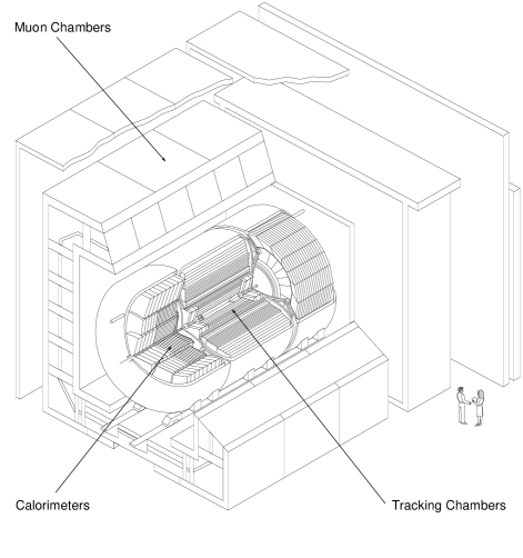
FIG. 3.: Cutaway view of the DØ detector

The innermost part of the detector consists of a set of tracking chambers that surround the beam pipe. There is no central magnetic field and jets are measured using a compact set of calorimeters positioned outside the tracking volume. To identify muons, an additional set of tracking chambers is located outside the calorimeter, with a measurement of muon momentum provided through magnetized iron toroids placed between the first two muon-tracking layers.

The full detector is about 13 m high $\times$ 11 m wide $\times$ 17 m long, with a total weight of about 5500 tons. The Tevatron beam pipe passes through the center of the detector, while the Main Ring beam pipe passes through the upper portion of the calorimetry, approximately 2 m above the Tevatron beam pipe. The coordinate system used in DØ is right-handed, with the $z$-axis pointing along the direction of the proton beam (southward) and the $y$-axis pointing up. The polar angle $\theta=0$ is along the proton beam direction, and the azimuthal angle $\phi=0$ along the eastward direction. Instead of $\theta$, we often use the pseudorapidity, $\eta=-\ln[\tan(\theta/2)]$. This quantity approximates the true rapidity $y=1/2\ln[(E+p_{z})/(E-p_{z})]$, when the rest mass is much smaller than the total energy.

A Central Detector

The tracking chambers and a transition radiation detector make up the central detector (CD). The main purpose of the CD is to measure the trajectories of charged particles and determine the $z$ position of the interaction vertex. This information can be used to determine whether an electromagnetic energy cluster in the calorimeter is caused by an electron or by a photon. Additional information such as the number of tracks and the ionization energy along the track ($dE/dx$) can be used to determine whether a track is caused by one or several closely spaced charged particles, such as a photon conversion.

The CD consists of four separate subsystems: the vertex drift chamber (VTX), the transition radiation detector (TRD), the central drift chamber (CDC), and two forward drift chambers (FDC). The full set of CD detectors fits within the inner cylindrical aperture of the calorimeters in a volume of radius $r$ = 78 cm and length $l$ = 270 cm. The system provides charged-particle tracking over the region $|\eta|<$ 3.2. The trajectories of charged particles are measured with a resolution of 2.5 mrad in $\phi$ and 28 mrad in $\theta$. From these measurements, the position of the interaction vertex along the $z$ direction is determined with a resolution of 6 mm.

The VTX is the innermost tracking chamber in the DØ detector, occupying the region $r=3.7$ cm to 16.2 cm. It is made of three mechanically independent concentric layers of cells parallel to the beam pipe. The innermost layer has sixteen cells while the outer two layers have thirty-two cells each.

The TRD occupies the space between the VTX and the CDC; it extends from $r=17.5$ cm to 49 cm. The TRD consists of three separate units, each containing a radiator (393 foils of 18 $\mu$m thick polypropylene in a volume filled with nitrogen gas) and an X-ray detection chamber filled with Xe gas. The TRD information is not used in this analysis.

The CDC is a cylindrical drift chamber, 184 cm along $z$, located between $r=49.5$ and $r=74.5$ cm, and provides coverage for $|\eta|<$ 1.2. It is made up of four concentric rings of 32 azimuthal cells per ring. Each cell contains seven sense wires (staggered by 200 $\mu$m relative to each other to help resolve left-right ambiguities), and two delay lines. The $r\phi$ position of a hit is determined via the drift time measured for the hit wire and the $z$ position of a hit is measured using inductive delay lines embedded in the module-walls of the sense wire planes.

The FDC consists of two sets of drift chambers located at the ends of the CDC. They perform the same function as the CDC, but for 1.4 $<|\eta|<$ 3.1. Each FDC package consists of three separate chambers: a $\Phi$ module, whose sense wires are radial and measure the $\phi$ coordinate, sandwiched between a pair of $\Theta$ modules whose sense wires measure the $\theta$ coordinate.

B Calorimeters

The DØ calorimeters are sampling calorimeters, with liquid argon as the sensitive ionization medium. The primary absorber material is depleted uranium, with copper and stainless steel used in the outer regions. There are three separate units, each contained in separate cryostats: the Central Calorimeter (CC), the North End Calorimeter (ECN), and the South End Calorimeter (ECS). The readout cells are arranged in a pseudo-projective geometry pointing to the interaction region.

The calorimeters are subdivided in depth into three distinct types of modules: electromagnetic sections (EM) with relatively thin uranium absorber plates, fine-hadronic sections (FH) with thicker uranium plates, and coarse-hadronic sections (CH) with thick copper or stainless steel plates. There are four separate layers for the EM modules in both the CC and EC that are readout separately. The first two layers are 2 radiation lengths thick in the CC and 0.3 and 2.6 radiation lengths thick in the EC, and measure the initial longitudinal shower development, where photons and $\pi^{0}$s differ somewhat on a statistical basis. The third layer spans the region of maximum EM shower energy deposition and the fourth completes the EM coverage of approximately 20 total radiation lengths. The fine-hadronic modules are typically segmented into three or four layers. Typical transverse sizes of towers in both EM and hadronic modules are $\Delta\eta=0.1$ and $\Delta\phi=2\pi/64\approx 0.1$. The third section of the EM modules is segmented twice as finely in both $\eta$ and $\phi$ to provide more precise determination of centroids of EM showers.

The CC has a length of 2.6 m, covering the pseudorapidity region $|\eta|<$ 1.2, and consists of three concentric cylindrical rings. There are 32 EM modules in the inner ring, 16 FH modules in the surrounding ring, and 16 CH modules in the outer ring. The EM, FH and CH module boundaries are rotated with respect to each other so as to prevent having more than one intermodular gap intercepting a trajectory from the origin of the detector.

The two end calorimeters (ECN and ECS) are mirror-images, and contain four types of modules. To avoid the dead spaces in a multi-module design, there is just a single large EM module and one inner hadronic (IH) module. Outside the EM and IH, there are concentric rings of 16 middle and outer hadronic modules (MH and OH). The azimuthal boundaries of the MH and OH modules are also offset to prevent cracks through which particles could penetrate the calorimeter. This makes the DØ detector almost completely hermetic and provides an accurate measurement of missing transverse energy. Due to increase in background and loss of tracking efficiency for $|\eta|>2.5$, electron and photon candidates are restricted to $1.5<|\eta|<2.5$ in the EC.

In the transition region between the CC and EC ($0.8\leq|\eta|\leq 1.4$), there is a large amount of uninstrumented material in the form of cryostat walls, stiffening rings, and module endplates. To correct for energy deposited in the uninstrumented material, we use two segmented (0.1 $\times$ 0.1 in $\eta\times\phi$) arrays of scintillation counters, called intercryostat detectors. In addition, separate single-cell structures called “massless gaps” are mounted on the end plates of the CC-FH modules and on the front plates of EC-MH and EC-OH modules, and are used to correct showers in this region of the detector.

The Main Ring beam pipe passes through the outer layers of the CC, ECN and ECS. Beam losses from the Main-Ring cause energy deposition in the calorimeter that can bias the energy measurement. The data acquisition system either stops recording data during periods of Main-Ring activity near the DØ detector, or flags such events.

C Muon Detectors

The DØ muon detector is designed to identify muons and to determine their trajectories and momenta. It is located outside of the calorimeter, and is divided in two subsystems: the Wide Angle Muon Spectrometer and the Small Angle Muon Spectrometer. Since the calorimeter is thick enough to absorb most of the debris from electromagnetic and hadronic showers, muons can be identified with great confidence. The muon system is not used in this analysis, and is therefore not discussed any further.

III Multilevel Trigger and Data Acquisition Systems

The DØ trigger system is a multilayer hierarchical system. Increasingly complex tests are applied to the data at each successive stage to reduce background.

The first stage, called Level 0 (L0), consists of two scintillator arrays mounted on the front surfaces of the EC cryostats, perpendicular to the beam direction. Each array covers a partial region of pseudorapidity for 1.9 $<|\eta|<$ 4.3, with nearly complete coverage over the range 2.2 $<|\eta|<$ 3.9. The L0 system is used to detect the occurrence of an inelastic $p{\bar{p}}$ collision, and serves as the luminosity monitor for the experiment. In addition, it provides fast information on the $z$-coordinate of the primary collision vertex, by measuring the difference in arrival time between particles hitting the north and south L0 arrays; this is used in making preliminary trigger decisions. A slower, more accurate measurement of the position of the interaction vertex, and an indication of the possible occurrence of multiple interactions, are also made available for subsequent trigger decisions. The L0 trigger is $\approx$ 99% efficient for non-diffractive inelastic collisions. The output rate from L0 is on the order of 150 kHz at a typical luminosity of $1.6\times 10^{31}{\rm cm}^{-2}$ ${\rm s}^{-1}$.

The next stage of the trigger is called Level 1 (L1). It combines the results from individual L1 components into a set of global decisions that command the readout of the digitization crates. It also interacts with the Level 2 trigger (L2). Most of the L1 components, such as the calorimeter triggers and the muon triggers, operate within the 3.5 $\mu s$ interval between beam crossings, so that all events are examined. However, other components, such as the TRD trigger and several components of the calorimeter and muon triggers, called Level 1.5 trigger (L1.5), can require more time. The goal of the L1 trigger is to reduce the event rate to 100–200 Hz. The primary input for the L1 trigger consists of 256 trigger terms, each of which corresponds to a single bit, indicating that some specific requirement is met. These 256 terms are reduced to a set of 32 L1 trigger bits by a two-dimensional AND-OR logic network. An event is said to pass L1 if at least one of these 32 bits is set. The L1 trigger also uses information based on Main Ring activity. To prevent saturation of the trigger system by processes with large cross sections, such as QCD multijet production, any particular contributor to the L1 trigger can be prescaled.

The L1 calorimeter trigger covers the region up to $|\eta|<$ 4.0 in trigger towers of 0.2 $\times$ 0.2 in $\eta-\phi$ space. These towers are subdivided longitudinally into electromagnetic and hadronic trigger sectors. The output of the L1 calorimeter trigger corresponds to the transverse energy deposited in these sectors and towers.

For the 1993–1995 collider run, an L1.5 trigger for the calorimeter was implemented using the L1 calorimeter trigger data and filters based on neighbor sums and ratios of the EM and total transverse energies.

When an event satisfies the L1 trigger, the data are passed on the DØ data acquisition pathways to a farm of 48 parallel microprocessors, which serve as event builders as well as the L2 trigger system. The L2 system collects the digitized data from all elements of the detector and trigger blocks for events that successfully pass Level 1. It applies sophisticated algorithms to the data to reduce the event rate to about 2 Hz before passing the accepted events on to the host computer for monitoring and recording. The data for a specific event are sent over parallel paths to memory modules in specific selected nodes. The accepted data are collected and formatted in final form in the nodes, and the L2 filter algorithms are then executed.

The L2 filtering process in each node is built around a series of filter tools. Each tool has a specific function related to the identification of a type of particle or event characteristic. There are tools to recognize jets, muons, calorimeter EM clusters, tracks associated with calorimeter clusters, $\sum E_{T}$ (sum of transverse energies of jets), and $\hbox to0.0pt{\kern 2.5pt/\hss}E_{T}$ (imbalance in transverse energy). Other tools recognize specific noise or background conditions. There are 128 L2 filters available. If all of the L2 requirements (for at least one of these 128 filters) are satisfied, the event is said to pass L2 and it is temporarily stored on disk before being transferred to an 8 mm magnetic tape.

Once an event is passed by an L2 node, it is transmitted to the host cluster, where it is received by the data logger, a program running on one of the host computers. This program and others associated with it are responsible for receiving data from the L2 system and copying it to magnetic tape, while performing all necessary bookkeeping tasks (e.g., time stamping, recording the run number, an event number, etc.). Part of the data is sent to an event pool for online monitoring.

A Electron Trigger

To trigger on electrons, L1 requires the transverse energy in the EM section of a trigger tower to be above a programmable threshold. The L2 electron algorithm then uses the full segmentation of the EM calorimeter to identify electron showers. Using the trigger towers that are above threshold at L1 as seeds, the algorithm forms clusters that include all cells in the four EM layers and the first FH layer in a region of $\Delta\eta\times\Delta\phi$ = 0.3 $\times$ 0.3, centered on the tower with the highest $E_{T}$. The longitudinal and transverse energy profile of the cluster must satisfy the following requirements: (i) the fraction of the cluster energy in the EM section (the EM fraction) must be above a threshold, which depends on energy and detector position; and (ii) the difference between the energy depositions in two regions of the third EM layer, covering $\Delta\eta\times\Delta\phi$ = 0.25 $\times$ 0.25 and 0.15 $\times$ 0.15, and centered on the cell with the highest $E_{T}$, must be within a window that depends on the total cluster energy.

B Jet Trigger

The L1 jet triggers require the sum of the transverse energy in the EM and FH sections of a trigger tower ($\Delta\eta\times\Delta\phi=0.2\times 0.2$) to be above a programmable threshold. The L2 jet algorithm begins with an $E_{T}$-ordered list of towers that are above threshold at L1. At L2, a jet is formed by placing a cone of given radius ${\cal R}$, where ${\cal R}=\sqrt{\Delta\eta^{2}+\Delta\phi^{2}}$, around the seed tower from L1. If another seed tower lies within the jet cone, it is passed over and not allowed to seed a new jet. The summed $E_{T}$ in all of the towers included in the jet cone defines the jet $E_{T}$. If any two jets overlap, then the towers in the overlap region are added into the jet candidate that is formed first. To filter out events, requirements on quantities such as the minimum transverse energy of a jet, the minimum transverse size of a jet, the minimum number of jets, and the pseudorapidity of jets, can be imposed at this point.

C Missing Transverse Energy Trigger

Rare and interesting physics processes often involve production of weakly interacting particles such as neutrinos. These particles usually can not be detected directly. However, assuming momentum conservation in a collision allows the momenta of such particles to be inferred from the vector sum of the momenta of the observed particles. Since the energy flow near the beamline is largely undetected, such calculations are realistic only in the plane transverse to the beam. The negative of the vector sum of the momenta of the detected particles is referred to as missing $E_{T}$ and denoted by $\hbox to0.0pt{\kern 2.5pt/\hss}E_{T}$; it is used as an indicator of the presence of weakly interacting particles. At L2, $\hbox to0.0pt{\kern 2.5pt/\hss}E_{T}$ is computed using the vector sum of all calorimeter and intercryostat detector cell energies with respect to the $z$ position of the interaction vertex, which is determined from the timing of the hits in the L0 counters.

IV Particle Identification

A Electron

Electrons and photons are identified by the properties of the shower in the calorimeter. The algorithm loops over all EM towers ($\Delta\eta\times\Delta\phi=0.1\times 0.1$) with energy $E>50$ MeV, and connects the neighboring tower with the next highest energy. The cluster energy is then defined as the sum of the energies of the EM towers and the energies in the corresponding first FH layer. The ratio of the energy in the EM cluster to the total energy (EM energy summed with the corresponding hadronic layers), defined as the EM fraction, is used to discriminate electrons and photons from hadronic showers. A cluster must pass the following criteria to be an electron/photon candidate: (i) the EM fraction must be greater than 90% and (ii) at least 40% of the energy must be contained in a single $0.1\times 0.1$ tower. To distinguish electrons from photons, we search for a track in the central detector that extrapolates to the EM cluster from the primary interaction vertex within a window of $|\Delta\eta|\leq 0.1$, and $|\Delta\phi|\leq 0.1$. If one or more tracks are found, the object is classified as an electron candidate. Otherwise, it is classified as a photon candidate.

1 Selection Requirements

The spatial development of EM showers is quite different from that of hadronic showers and the shower shape information can be used to differentiate electrons and photons from hadrons. The following variables are used for final electron selection:

(i) Electromagnetic energy fraction. This quantity is based on the observation that electrons deposit almost all of their energy in the EM section of the calorimeter, while hadron jets are far more penetrating (typically only 10% of their energy is deposited in the EM section of the calorimeter). It is defined as the ratio of EM energy to the total shower energy. Electrons are required to have at least 95% of their total energy in the EM calorimeter. This requirement loses only about 1% of all electrons.

(ii) Covariance matrix ($H$-matrix) $\chi^{2}$. The shape of any shower can be characterized by the fraction of the cluster energy deposited in each layer and tower of the calorimeter. These fractions are correlated, i.e., an electron shower deposits energies according to the expected transverse and longitudinal shapes of an EM shower and a hadron shower following the typical development of a hadronic shower. To obtain good discrimination against hadrons, we use a covariance matrix technique. The observables in this method are the fractional energies in Layers 1, 2, and 4 of the EM sector and the fractional energy in each cell of a $6\times 6$ array of cells in Layer 3 centered on the most energetic tower in the EM cluster. To take account of the dependence of the shower shape on energy and on the position of the primary interaction vertex, we use the logarithm of the shower energy and the z-position of the event vertex as the remaining input observables. The event vertex is determined by extrapolating CDC tracks to the $z$ axis, and for more than one possibility, the vertex associated with the highest number of tracks is chosen as the event vertex. Using these 41 variables, covariance matrices are constructed for each of the 37 detector towers (at different values of $\eta$) based on Monte Carlo generated electrons. The Monte Carlo showers are tuned to make them agree with our test beam measurements of the shower shapes. The 41 observables for any given shower can be compared with the parameters of the appropriate covariance matrix to define a $\chi^{2}$, which is to be be less than 100 for electron candidates in the CC and less than 200 for the EC. This requirement loses about 5% of all true electrons.

(iii) Isolation. The decay electron from a $W$ boson should not be close to any other object in the event. This is quantified by the isolation fraction. If $E(0.4)$ is the energy deposited in all calorimeter cells within the cone ${\cal R}<0.4$ around the direction of the electron, and $EM(0.2)$ is the energy deposited in only the EM calorimeter in the cone ${\cal R}<0.2$, the isolation variable is then defined as the ratio ${\cal I}=[E(0.4)-EM(0.2)]/EM(0.2).$ The requirement ${\cal I}<0.1$ loses only 3% of the electrons from $W$ boson decays.

(iv) Track-match significance. An important source of background for electrons is the photon from the decay of $\pi^{0}$ or $\eta$ mesons. Such photons do not produce tracks, but their trajectories can overlap with those of nearby charged particles, thereby simulating electrons. This background can be reduced by demanding a good spatial match between the energy cluster in the calorimeter and nearby charged tracks. The significance $S$ of the mismatch between these quantities is given by $S=[({\Delta\phi}/{\delta_{\Delta\phi}})^{2}+({\Delta z}/{\delta_{\Delta z}})^{2}]^{1/2}$, where $\Delta\phi$ is the azimuthal mismatch, $\Delta z$ the mismatch along the beam axis, and the $\delta$ are the resolutions of these variables. This form for $S$ is appropriate for the central calorimeter. For the end calorimeter, $r$ replaces $z$. Requiring $S<5$ accepts 95(78)% of the CC(EC) electrons reconstructed in the central tracker.

(v) Track-in-road. All electrons from $W\rightarrow e\nu$ decays are required to have a partially reconstructed track along the trajectory between the energy cluster in the calorimeter and the interaction vertex. This requirement is found to reject 16(14)% of CC(EC) electrons from $W$ boson decay.

In our analysis, we combine the above quantities to form the electron identification criteria. A summary of the selection requirements and their acceptance efficiencies is listed in Table I (See SectVII).

TABLE I.: Electron selection requirements and their acceptance efficiencies for $W\rightarrow e\nu$ events.

Selection	CC		EC
requirement		$\varepsilon$		$\varepsilon$
$H$-matrix $\chi^{2}$	$<100$	0.946$\pm$0.005	$<200$	0.950$\pm$0.008
EM fraction	$>0.95$	0.991$\pm$0.003	$>0.95$	0.987$\pm$0.006
Isolation	$<0.10$	0.970$\pm$0.004	$<0.10$	0.976$\pm$0.007
Track match	$<5$	0.948$\pm$0.005	$<5$	0.776$\pm$0.012
Track-in-road		0.835$\pm$0.009		0.858$\pm$0.006

2 Electromagnetic Energy Corrections

The energy scales of the calorimeters were originally set through calibration in a test-beam. However, due to differences in conditions between the test beam and the DØ environment, additional corrections had to be implemented.

The EM energy scales for the calorimeters were determined by comparing the measured masses of $\pi^{0}\rightarrow\gamma\gamma$, $J/\psi\rightarrow ee$, and $Z\rightarrow ee$ to their known values. If the electron energy measured in the calorimeter and the true energy are related by $E_{\rm meas}=\alpha E_{\rm true}+\delta$, the measured and true mass values are, to first order, related by $m_{\rm meas}=\alpha m_{\rm true}+\delta f$, where the calculable variable $f$ reflects the topology of the decay. To determine $\alpha$ and $\delta$, we fit the Monte Carlo prediction to the observed resonances, with $\alpha$ and $\delta$ as free parameters [22]. The values of $\alpha$ and $\delta$ are found to be $\alpha=0.9533\pm 0.0008$ and $\delta=-0.16^{+0.03}_{-0.21}$ GeV for the CC and $\alpha=0.952\pm 0.002$ and $\delta=-0.1\pm 0.7$ GeV for the EC.

3 Energy Resolution

The relative energy resolution for electrons and photons in the CC is expressed by the empirical relation $\left(\frac{\sigma}{E}\right)^{2}=C^{2}+\frac{S^{2}}{E_{T}}+\frac{N^{2}}{E^{2}}$, where $E$ and $E_{T}$ are the energy and transverse energy of the incident electron/photon, $C$ is a constant term from uncertainties in calibration, $S$ reflects the sampling fluctuation of the liquid argon calorimeter, and $N$ corresponds to a contribution from noise. For the EC, the $E_{T}$ in the relation is replaced by $E$. The sampling and noise terms are based on results from the test beam. The noise term measured at the test beam agrees with the one obtained in the collider environment (based on the width of pedestal distributions). The constant term is tuned to match the mass resolution of both observed and simulated $Z\rightarrow ee$ events. Table II lists these parameters.

TABLE II.: Parameters for describing the energy resolution of electrons and photons.

Quantity	CC	EC
$C$	0.017	0.009
$S$ ($\sqrt{\rm GeV}$)	0.14	0.157
$N$ (GeV)	0.49	1.140

B Jets

In our analysis, jets are reconstructed using a fixed-cone algorithm with radius ${\cal R}=\sqrt{\Delta\eta^{2}+\Delta\phi^{2}}=0.5$. The algorithm forms preclusters of contiguous cells using a radius of ${\cal R}_{\rm precluster}=0.3$ centered on the tower with highest $E_{T}$. Only towers with $E_{T}>$ 1 GeV are included in preclusters. These preclusters serve as the starting points for jet reconstruction. An $E_{T}$-weighted center of gravity is then formed using the $E_{T}$ of all towers within a radius ${\cal R}$ of the center of the cluster, and the process is repeated until the jet becomes stable. A jet must have $E_{T}>$ 8 GeV. If two jets share energy, they are combined or split, based on the fraction of overlapping energy relative to the $E_{T}$ of the lesser jet. If this shared fraction exceeds 50%, the jets are combined.

Although the ${\cal R}=0.3$ cone algorithm is more efficient for jet finding than our larger cone size, which leads to undesired merging of jets for high-$p_{T}$ $W$ or $Z$ bosons, the relatively large uncertainties in the measurement of jet-energy for the ${\cal R}=0.3$ cones negate their advantage, and we therefore choose to use the ${\cal R}=0.5$ cone algorithm for our studies.

1 Selection Requirements

To remove jets produced by cosmic rays, calorimeter noise, and interactions in the Main Ring, we developed a set of requirements based on Monte Carlo studies of jets in such environments and on data on noise taken with and without colliding beams. The variables used are:

(i) Electromagnetic energy fraction ($emf$). As for electrons, this quantity is defined as the fraction of the total energy deposited in the electromagnetic section of the calorimeter. A requirement on this quantity removes electrons, photons and false jets from the jet sample. Electrons and photons typically have a high EM fraction. False jets are caused mainly by background from the Main Ring or by noisy or “hot” cells, and therefore generally do not contain energy in the EM section, thereby yielding very low EM fractions. Jets with $0.05<emf<0.95$ are defined as acceptable in this analysis. The efficiency of this requirement is 99.9% at $E_{T}=20$ GeV and decreases to 99.6% at 100 GeV.

(ii) Hot cell energy fraction ($hcf$). The $hcf$ is defined as the ratio of the energy in the cell of second highest $E_{T}$ to that of the cell with highest $E_{T}$ within a jet. A requirement on this quantity is imposed to remove events with a large amount of noise in the calorimeter. Hot cells can appear when a discharge occurs between electrodes within a cell; often this does not affect neighboring cells. In this case, $hcf$ is small, which signals a problem, since the $hcf$ for a jet should not be small because the energy is expected to be distributed over cells. If most of the energy is concentrated in a single cell, it is very likely to be a false jet reconstructed from discharge noise. For good jets, $hcf$ is found to be greater than 0.1. The efficiency of this requirement is 97.3% at $E_{T}=20$ GeV and decreases to 96.9% at 100 GeV.

(iii) Coarse hadronic energy fraction ($chf$). This quantity is defined as the fraction of jet energy deposited in the coarse hadronic section of the calorimeter. The Main Ring at DØ passes through the CH modules, and any energy deposition related to the Main Ring will be concentrated in this section of the calorimeter. Such jets tend to have more than 40% of their energy in the CH region, while standard jets have less than 10% of their energy in this section of the calorimeter. All acceptable jets are therefore required to have $chf<0.4$. The efficiency of this requirement is 99.6% at $E_{T}=20$ GeV and decreases to 99.3% at 100 GeV.

2 Hadronic Energy Corrections

Since the measured jet energy is usually not equal to the energy of the original parton that formed the jet, corrections are needed to minimize any systematic bias. Jet energy response affected by non-uniformities in the calorimeter, non-linearities in the response to hadrons, emission of particles outside of the ${\cal R}=0.5$ cone (often referred to as out-of-cone showering), noise due to the radioactivity of uranium, and energy overlap from the products of soft interactions of spectator partons within the proton and the antiproton (“underlying event”). The first two effects are estimated using a method called Missing-$E_{T}$ Projection Fraction (MPF) [23].

The MPF method is based on events that contain a single isolated EM cluster (due to a photon or a jet that fragmented mostly into neutral mesons), and one hadronic jet located opposite in $\phi$, and no other objects in the event. It is assumed that such events do not have energetic neutrinos so that any missing transverse energy can be attributed to a mismeasurement of the hadronic jet. The EM-cluster energy is corrected using the electromagnetic energy corrections described above. Projecting the corrected $\hbox to0.0pt{\kern 2.5pt/\hss}E_{T}$ along the jet axis determines corrections to the jet energy. This correction is averaged over many events in the sample to obtain a correction as a function of jet $E_{T}$, $\eta$, and electromagnetic content of the jet. The hadronic energy correction is 20% at $E=20$ GeV and 15% at $E=100$ GeV, and gradually approaches 10% at high $E$.

The impact of out-of-cone showering is estimated using Monte Carlo jet events. Effects due to the underlying events and uranium noise are determined in separate studies using minimum-bias event data. (Minimum-bias data corresponds to inclusive inelastic collisions collected using only the L0 trigger.)

3 Energy Resolution

The jet energy resolution has been studied by examining momentum balance in dijet events [24]. The formula used for parametrizing the relative jet energy resolution is $\left(\frac{\sigma}{E}\right)^{2}=C^{2}+\frac{S^{2}}{E}+\frac{N^{2}}{E^{2}}$. Table III shows the values of the parameters for different $\eta$ regions of the calorimeter.

TABLE III.: Jet energy resolution for different regions of the calorimeter.

$\eta$ Region	$C$		$S$ ($\sqrt{\rm GeV}$)		$N$ (GeV)
$|\eta|<$ 0.5	0.00$\pm$	0.01	0.81$\pm$	0.02	7.07$\pm$	0.09
0.5 $<|\eta|<$ 1.0	0.00$\pm$	0.01	0.91$\pm$	0.02	6.92$\pm$	0.09
1.0 $<|\eta|<$ 1.5	0.05$\pm$	0.01	1.45$\pm$	0.02	0.00$\pm$	1.40
1.5 $<|\eta|<$ 2.0	0.00$\pm$	0.01	0.48$\pm$	0.07	8.15$\pm$	0.21
2.0 $<|\eta|<$ 3.0	0.01$\pm$	0.58	1.64$\pm$	0.13	3.15$\pm$	2.50

C Neutrinos: Missing Transverse Energy

The presence of neutrinos in an event is inferred from the $\hbox to0.0pt{\kern 2.5pt/\hss}E_{T}$. In this analysis we assume that the $\hbox to0.0pt{\kern 2.5pt/\hss}E_{T}$ in each candidate event corresponds to the neutrino from the decay $W\rightarrow e\nu$.

1 Missing $E_{T}$

The missing transverse energy in the calorimeter is defined as $\hbox{$\hbox to0.0pt{\kern 2.5pt/\hss}E_{T}$}=(\hbox{$\hbox to0.0pt{\kern 2.5pt/\hss}E_{T}$}_{x}^{2}+\hbox{$\hbox to0.0pt{\kern 2.5pt/\hss}E_{T}$}_{y}^{2})^{1/2}$, where $\hbox{$\hbox to0.0pt{\kern 2.5pt/\hss}E_{T}$}_{x}=-\sum_{i}E_{i}\sin(\theta_{i})\cos(\phi_{i})-\sum_{j}\Delta E_{x}^{j}$ and $\hbox{$\hbox to0.0pt{\kern 2.5pt/\hss}E_{T}$}_{y}=-\sum_{i}E_{i}\sin(\theta_{i})\sin(\phi_{i})-\sum_{j}\Delta E_{y}^{j}$. The first sum (over $i$) is over all cells in the calorimeters, intercryostat detectors and massless gaps (see Sec. II B). The second sum (over $j$) is over the $E_{T}$ corrections applied to all electrons and jets in the event. This can be used to estimate the transverse momentum of any neutrinos in an event that does not contain muons, which deposit only a small portion of their energy in the calorimeter. The total missing $E_{T}$ is missing $E_{T}$ from the calorimeter corrected for the transverse momenta of any observed muon tracks. Since this analysis does not use muons, we will refer to the $\hbox to0.0pt{\kern 2.5pt/\hss}E_{T}$ based on the calorimeters as the true $\hbox to0.0pt{\kern 2.5pt/\hss}E_{T}$.

2 Resolution in $\hbox to0.0pt{\kern 2.5pt/\hss}E_{T}$

For an ideal calorimeter, the magnitude of the components of the $\hbox to0.0pt{\kern 2.5pt/\hss}E_{T}$ vector would sum to zero for events with no true source of $\hbox to0.0pt{\kern 2.5pt/\hss}E_{T}$. However, detector noise and energy resolution in the measurement of jets, photons, and electrons contribute to the $\hbox to0.0pt{\kern 2.5pt/\hss}E_{T}$. In addition, non-uniform response in the detector also results in $\hbox to0.0pt{\kern 2.5pt/\hss}E_{T}$. The $\hbox to0.0pt{\kern 2.5pt/\hss}E_{T}$ resolution for our candidate events is parameterized as $\sigma=1.08{\rm GeV}+0.019(\sum E_{T})$, and is based on studies of minimum-bias data [24]. The $\sum E_{T}$ used in the parameterization is quite reasonable because the greater the total amount of transverse energy in the event, the larger the possibility for its mismeasurement.

V Data Sample

The analysis of the $WW/WZ\rightarrow e\nu jj$ process is based on data taken during the 1993–1995 Tevatron Collider run (called Run 1b). The L0 trigger is used to check the presence of an inelastic collision, but is not included in the trigger conditions for $W$-boson data. This was done to allow studies of diffractive $W$-boson production. Our analysis uses the collected $W\rightarrow e\nu$ data sample, with the L0 trigger requirement imposed offline. The L1 trigger used in this analysis (called the EM1_1_HIGH trigger) requires the presence of an electromagnetic trigger tower with $E_{T}>10$ GeV. The L1.5 trigger then requires the L1 trigger tower to have $E_{T}>15$ GeV and checks that the electromagnetic fraction is greater than 85%. The L2 component of the trigger (called the EM1_EISTRKCC_MS trigger) requires an isolated electron candidate with $E_{T}>20$ GeV that has a shower shape consistent with that of an electron and $\hbox{$\hbox to0.0pt{\kern 2.5pt/\hss}E_{T}$}>15$ GeV.

Additional conditions are imposed on the data to further reduce background. Triggers that occur at the times when a proton bunch in the Main Ring passes through the detector are not used in this analysis. Similarly, triggers that occur during the first 0.4 seconds of the 2.4-second antiproton production cycle are rejected. Data taken during periods when the data acquisition system or the detector sub-systems malfunctioned are also discarded. With these trigger requirements, the integrated luminosity of the data sample is estimated to be $82.3\pm 4.4$ ${\rm pb}^{-1}$ [25]. The efficiency and turn-on of the L2 trigger are described in Ref. [26]. The trigger efficiency for signal is ($98.1\pm 1.9$)%.

Data samples that satisfy two other L2 triggers, the EM1_ELE_MON and ELE_1_MON triggers, are used for background studies. These triggers select events that have an electron candidate with $E_{T}>20$ GeV and $E_{T}>16$ GeV, respectively. The electron candidates in these samples must pass the standard shower-shape requirements, but not the isolation requirement. These triggers use the same L1 and L1.5 conditions as the trigger used for signal.

VI Event Selection

$WW/WZ\to e\nu jj$ candidates are selected by searching for events with an isolated high-$E_{T}$ electron, large $\hbox to0.0pt{\kern 2.5pt/\hss}E_{T}$, and at least two high-$E_{T}$ jets. Electrons in the candidate sample must be in the $|\eta|<1.1$ region but away from the boundaries between calorimeter modules in $\phi$ ($\Delta\phi>0.01$), or within the region $1.5<|\eta|<2.5$. Jets in the candidate sample must be in the region $|\eta|<2.5$.

The $W\rightarrow e\nu$ decay is defined through the presence of only a single isolated electron with $E_{T}^{e}>25$ GeV and $\hbox{$\hbox to0.0pt{\kern 2.5pt/\hss}E_{T}$}>25$ GeV in the event. The transverse mass of the electron and neutrino ($\hbox to0.0pt{\kern 2.5pt/\hss}E_{T}$) system is required to be $M_{T}>40$ GeV/$c^{2}$, where $M_{T}=\{2E_{T}^{e}\hbox{$\hbox to0.0pt{\kern 2.5pt/\hss}E_{T}$}[1-\cos(\phi_{e}-\phi_{\nu})]\}^{1/2}$. The requirement on the electron $E_{T}$ is sufficiently high to provide an efficiency that is independent of $E_{T}$ (the hardware threshold of $20$ GeV). Requiring only one electron reduces background from $Z\rightarrow ee$ production. The requirements on $\hbox to0.0pt{\kern 2.5pt/\hss}E_{T}$ and $M_{T}$ reduce the background contribution from misidentified electrons.

The $W/Z\rightarrow jj$ decay is defined by requiring at least two jets with $E^{j}_{T}>20$ GeV and an invariant mass of the two-jet system consistent with that of the $W$ or $Z$ boson ($50<M_{jj}<110$ GeV/$c^{2}$). The dijet invariant mass ($M_{jj}$) is calculated via $M_{jj}=\{2E_{T}^{j1}E_{T}^{j2}[\cosh(\eta_{j1}-\eta_{j2})-\cos(\phi_{j1}-\phi_{j2})]\}^{1/2}$. If there are more than two jets in the event, the two jets with the highest dijet invariant mass are chosen to represent the $W$ (or $Z$) decay.

The difference between the $p_{T}$ values of the $e\nu$ and the two-jet systems is used to reduce backgrounds. For $WW$ or $WZ$ production, the $p_{T}(e\nu)-p_{T}(jj)$ distribution should be peaked near zero and have a symmetric Gaussian shape, with the width of the Gaussian distribution determined primarily by the jet energy resolution. On the other hand, for background such as $t\bar{t}$ production (see Sec. VIII), the distribution should be broader and asymmetric (shifted to positive values) due to additional $b$-quark jets in the events. Our analysis therefore requires $|p_{T}(e\nu)-p_{T}(jj)|<40$ GeV/$c$.

The data satisfying the above selection criteria yield 399 events. Figure 4a shows a scatter plot of $p_{T}(e\nu)$ vs $p_{T}(jj)$ for candidate events that satisfy the two-jet mass requirement. The width of the band reflects both the resolution and the true spread in the $p_{T}$ values. Figure 4b shows a scatter plot of $p_{T}(e\nu)$ vs $M_{jj}$ without the imposition of the two-jet mass requirement.

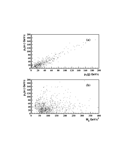
FIG. 4.: Scatter plots of (a) $p_{T}(e\nu)$ vs $p_{T}(jj)$ and (b) $p_{T}(e\nu)$ vs $M_{jj}$.

VII Detection Efficiency

A Electron Selection Efficiency

The efficiency of electron selection is studied using the $Z\rightarrow ee$ event sample from the 1993–1995 Tevatron collider run using the EM2_EIS_HI trigger. $Z\rightarrow ee$ events were selected at L1 and L1.5 by requiring two EM towers with $E_{T}>7$ GeV at L1, and at least one tower with $E_{T}>12$ GeV with more than $85$% of its energy in the EM section of the calorimeter. At L2, the trigger required two electron candidates with $E_{T}>20$ GeV that satisfied electron shower-shape and isolation requirements. To select an unbiased sample of electrons, we use events in which one of the electrons passes the tag quality requirements: EM fraction $>0.90$, Isolation $<0.15$, $H$-matrix $\chi^{2}<$ 100(200) for CC(EC), and track-match significance $<10$. The second electron in the event is then assumed to be unbiased. If both electrons pass the tag requirements, the event contributes twice to the sample. The efficiency of a selection requirement for electrons is given by $\varepsilon=(\varepsilon_{s}-\varepsilon_{b}f_{b})/(1-f_{b})$, where $\varepsilon_{s}$ is the efficiency measured in the signal region, $\varepsilon_{b}$ is the efficiency measured in the background region, and $f_{b}$ is the ratio of the number of background events in the signal region to the total number of events in the signal region. The signal region is defined as the region of the $Z$ mass peak ($86<m_{ee}<96$ GeV/$c^{2}$), and the background regions are defined as $61<m_{ee}<71$ GeV/$c^{2}$ and $111<m_{ee}<121$ GeV/c². We determine $f_{b}$ in the region of the signal using an average of the number of events in the background regions. The systematic uncertainties on the efficiencies are estimated from a comparison with efficiencies obtained using an alternative method that fits the invariant mass spectrum of two electrons to the sum of a Breit-Wigner form convoluted with a Gaussian and a linear dependence for the background. Efficiencies from the two methods agree within their uncertainties. The track-in-road efficiency is estimated in a similar manner, except that EM clusters with no matching track are included as unbiased electrons in the sample. Table I summarizes the electron efficiencies. Although these efficiencies are based mainly on $Z$ events with few jets, the corrections for $\geq 2$ jets are small.

B $W/Z\rightarrow jj$ Selection Efficiency

The $W/Z\rightarrow jj$ selection efficiency is estimated using Monte Carlo $WW/WZ\rightarrow e\nu jj$ events generated with the isajet [27] and pythia [28] programs, followed by a detailed simulation of the DØ detector, and parametrized as a function of $p^{W}_{T}$. Figure 5 shows the $W/Z\rightarrow jj$ detection efficiency $\epsilon(W\rightarrow jj)$ calculated as the ratio of events after the imposition of the two-jet selection requirements relative to the initial number of events. At low $p_{T}$, the detection efficiency is artificially elevated due to the presence of additional jets from initial- and final-state gluon radiation (ISR/FSR) that are mislabeled as being decays of $W$ or $Z$ bosons. The decrease in the efficiency at high $p_{T}$ is due to the merging of the two jets from a $W$ or a $Z$ boson. The results obtained from isajet are used to estimate the efficiencies for identifying the $WW/WZ$ process.

FIG. 5.: Efficiency for $W\rightarrow jj$ selection as a function of $p^{W}_{T}$. The decrease in the efficiency at high $p_{T}$ is due to the merging of the two jets from the decay of a $W$ boson.

The estimated $W/Z\rightarrow jj$ efficiency is affected by the jet energy scale, the accuracy of the ISR/FSR simulation, the accuracy of the parton fragmentation mechanism, and the statistics of the Monte Carlo samples.

The energy-scale correction has an uncertainty that decreases from 5% at jet $E_{T}=20$ GeV to 2% at 80 GeV, and then increases to 5% at 350 GeV. The effect of this uncertainty has been studied by recalculating the efficiency with the jet energy scale changed by one standard deviation. The largest relative change in the accepted number of events is found to be 3%.

To estimate the uncertainty due to the accuracy of the ISR/FSR simulation and of the parton fragmentation mechanism, we use the $W/Z\rightarrow jj$ efficiency based on Monte Carlo samples generated with pythia. The efficiency obtained using isajet is lower than that for pythia, but by less than 10%. We use the efficiencies from isajet because they provide smaller yields of $WW/WZ$ events and therefore weaker limits on anomalous couplings. We define one-half of the largest difference in isajet/pythia efficiency estimations (5%) as the systematic uncertainty attributable to the choice of event generator.

C Overall Selection Efficiency

The overall detection efficiency for $WW/WZ\rightarrow e\nu jj$ events assuming SM couplings is calculated using two MC methods, coupled with electron-selection and trigger efficiencies measured from data. The first MC method uses the isajet event generator followed by a detailed simulation of the DØ detector. The second MC method uses the event generator of Ref. [3] and a fast simulation program to characterize the response of the detector. isajet used the CTEQ2L [29] parton distribution functions to simulate 2500 $WW\rightarrow e\nu jj$ events and 1000 $WZ\rightarrow e\nu jj$ events with SM couplings. The event selection efficiency for for the $WW\rightarrow e\nu jj$ signal is estimated as $\epsilon_{WW}=(13.4\pm 0.8)$%, and $\epsilon_{WZ}=(15.7\pm 1.4)$% for the $WZ\rightarrow e\nu jj$ signal, where the errors are statistical. The combined efficiency for $WW/WZ\rightarrow e\nu jj$ is given by $[\epsilon_{WW}\cdot\sigma\cdot B(WW\rightarrow e\nu jj)+\epsilon_{WZ}\cdot\sigma\cdot B(WZ\rightarrow e\nu jj)]/[\sigma\cdot B(WW\rightarrow e\nu jj)+\sigma\cdot B(WZ\rightarrow e\nu jj)]=(13.7\pm 0.7)\%$, where the theoretical cross sections of 9.5 pb for $WW$ and 2.5 pb for $WZ$ production [30], and the $W$ and $Z$ boson branching fractions from the Particle Data Group [5], are used in the calculation ($\sigma\cdot B(WW\rightarrow e\nu jj)=1.38\pm 0.05$ pb and $\sigma\cdot B(WZ\rightarrow e\nu jj)=0.188\pm 0.006$ pb).

For the fast simulation, we generated over 30,000 events, with approximately four times more for $WW$ production than $WZ$ production, reflecting the sizes of their expected production cross sections. The overall detection efficiencies for the SM couplings were calculated as $[14.7\pm 0.2({\rm stat})\pm 1.2({\rm sys})]$% for $WW\rightarrow e\nu jj$ and $[14.6\pm 0.4({\rm stat})\pm 1.1({\rm sys})]$% for $WZ\rightarrow e\nu jj$. The 7.8% systematic uncertainty includes statistics of the fast MC (1%), efficiency of trigger and electron identification (1%), $\hbox to0.0pt{\kern 2.5pt/\hss}E_{T}$ smearing and modeling of the $p_{T}$ of the $WW/WZ$ system (5%), difference in $W\rightarrow jj$ detection efficiencies from the two event generators (5%), and the effect of the jet energy scale (3%). The combined efficiency is $[14.7\pm 0.2({\rm stat})\pm 1.2({\rm sys})]$%. The combined efficiency estimated using the fast simulation is consistent with the value obtained using isajet.

D Expected Number of Signal Events

Using the fast detector simulation and the cross section times branching ratio from the event generator of Ref. [3] ($\sigma\cdot B(WW\rightarrow e\nu jj)$ = 1.26 $\pm$ 0.18 pb, and $\sigma\cdot B(WZ\rightarrow e\nu jj)$ = 0.18 $\pm$ 0.03 pb), we estimate the number of expected $WW/WZ\rightarrow e\nu jj$ events to be 17.5 $\pm$ 3.0 (15.3 $\pm$ 3.0 $WW$ events and 2.2 $\pm$ 0.5 $WZ$ events), with the uncertainty (17.1%) given by the sum in quadrature of the uncertainty in the efficiency, the uncertainty in the luminosity (5.4%), and that in the NLO calculation (14%).

VIII Background

The sources of background to the $WW/WZ\rightarrow e\nu jj$ process can be divided into two categories. The first is instrumental background due to misidentified or mismeasured particles, and the other is inherent irreducible background consisting of physical processes with the same signature as the events of interest.

A Instrumental Background

The major source of instrumental background is QCD multijet production in which one of the jets showers (mainly) in the electromagnetic calorimeter and is misidentified as an electron, and the energies of the remaining jets fluctuate to produce $\hbox to0.0pt{\kern 2.5pt/\hss}E_{T}$. Although the probability for a jet to be misidentified as an electron is small, the large cross section for QCD multijet events makes this background significant.

This background is estimated using samples of “good” and “bad” electrons. A “good” electron has the quality requirements described in Sec. IV A 1, while a “bad” electron has an EM cluster with EM fraction $>$ 0.95, Isolation $\leq$ 0.15, and either $H$-matrix $\chi^{2}$ $\geq$ 250 or track-match significance $\geq$ 10. We assume that the shape of the $\hbox to0.0pt{\kern 2.5pt/\hss}E_{T}$ spectrum of the events with a bad electron is identical to the $\hbox to0.0pt{\kern 2.5pt/\hss}E_{T}$ spectrum of the QCD multijet background. Furthermore, with the assumption that the contribution of signal events at low $\hbox to0.0pt{\kern 2.5pt/\hss}E_{T}$ is negligible, the bad-electron sample can be normalized to the good-electron data in the low-$\hbox to0.0pt{\kern 2.5pt/\hss}E_{T}$ region and the $\hbox to0.0pt{\kern 2.5pt/\hss}E_{T}$ distribution of the bad-electron events can then be extrapolated to the signal region of the good-electron sample.

To estimate the multijet background, we use triggers that do not require $\hbox to0.0pt{\kern 2.5pt/\hss}E_{T}$. Several L2 triggers in Run 1b meet this requirement, in particular the triggers EM1_ELE_MON and ELE_1_MON described in Sec. V. To avoid biases, we add a condition that the EM object in these triggers pass the same L2 requirements as the signal. We then extract two samples from these data, based on the electron quality. The $\hbox to0.0pt{\kern 2.5pt/\hss}E_{T}$ distribution for the bad-electron sample is then normalized to agree with the $\hbox to0.0pt{\kern 2.5pt/\hss}E_{T}$ distribution for the good-electron sample at low $\hbox to0.0pt{\kern 2.5pt/\hss}E_{T}$ ($\hbox{$\hbox to0.0pt{\kern 2.5pt/\hss}E_{T}$}<15$ GeV). Figure 6 shows these two distributions. The normalization factor $N_{F}$ is calculated as the ratio of the number of bad-electron events to the number of good-electron events with $0\leq$ $\hbox to0.0pt{\kern 2.5pt/\hss}E_{T}$ $\leq 15$ GeV. After imposing the jet selection requirements on the events, we find $N_{F}$ = 1.870 $\pm$ 0.060 (stat) $\pm$ 0.003 (sys). The systematic uncertainty on the normalization factor is obtained by varying the range of $\hbox to0.0pt{\kern 2.5pt/\hss}E_{T}$ used for the normalization procedure from 0–12 GeV to 0–18 GeV.

FIG. 6.: $\hbox to0.0pt{\kern 2.5pt/\hss}E_{T}$ distributions for the good-electron (histogram) and bad-electron (solid circles) samples selected from data taken with the EM1_ELE_MON and ELE_1_MON triggers (see text). The bad-electron sample is normalized to the good electron sample for $\hbox{$\hbox to0.0pt{\kern 2.5pt/\hss}E_{T}$}<15$ GeV.

In the next step, we select two samples from the data taken with the trigger for signal events, one containing background and signal (“good” electrons obtained through our selection procedure) and the other containing only background events (“bad” electrons). The normalization factor $N_{F}$ is then applied to the background sample. Figure 7 shows the distributions of $\hbox to0.0pt{\kern 2.5pt/\hss}E_{T}$ for the candidates and the estimated QCD multijet background based on the bad-electron events after the imposition of jet requirements.

FIG. 7.: Distributions of $\hbox to0.0pt{\kern 2.5pt/\hss}E_{T}$ of the good-electron (sum of signal and background) and bad-electron (background only) samples selected from data taken with the trigger used for signal events.

From the above procedure, we estimate 104.3 $\pm$ 8.2 (stat) $\pm$ 9.1 (sys) background events for $\hbox{$\hbox to0.0pt{\kern 2.5pt/\hss}E_{T}$}>25$ GeV. The systematic uncertainty (8.7%) includes the uncertainty on the normalization factor (1%), the difference when an alternative method is used to estimate the multijet background (5.2%), and the difference for events with $\hbox to0.0pt{\kern 2.5pt/\hss}E_{T}$ $>25$ GeV when the $\hbox to0.0pt{\kern 2.5pt/\hss}E_{T}$ region 15–25 GeV is used for normalization (6.9%). In the alternative method, the probability of a jet to be misidentified as an electron is multiplied by the number of multijet events that satisfy selection criteria when one of the jets in the event is treated as an electron. When more than one jet in an event satisfies the kinematic requirements, all are considered in estimating the background from multijet production.

B Inherent Background

The background contribution from processes with similar event topology (i.e., with final-state objects identical to those of the signal) is estimated using Monte Carlo events.

1 $W+\geq$ 2 jets

$W+\geq$ 2 jets production is the dominant background to the $WW$ and $WZ$ signals. This background is estimated using the Monte Carlo program vecbos [31], followed by herwig [32] for the hadronization of the partons generated in vecbos and then by the detailed simulation of the DØ detector. The cross section from vecbos has a large uncertainty, and the generated $W+\geq 2$ jets sample is therefore normalized to the candidate event sample after subtraction of the QCD multijet background. To avoid the inclusion of $WW$ and $WZ$ events in this normalization procedure, we use only the events whose two-jet invariant mass lies outside of the mass peak of the $W$ boson (i.e., $M_{jj}>50$ or $M_{jj}>110$ GeV/$c^{2}$). Figure 8 shows the two-jet invariant mass distributions for data and the estimated background. The normalization factor is found to be $N_{V}=N_{VB}/(N_{\rm cand}-N_{\rm QCD}/N_{F})=3.41\pm 0.31({\rm stat})\pm 0.29({\rm syst})$, where $N_{VB}=879$ corresonds to the number of vecbos events, $N_{\rm cand}=392$ is the number of candidate events in the data, and $N_{\rm QCD}=251$ is the number of QCD multijet events outside of the $W$ boson mass window. Using this normalization factor, we estimate 279.5 $\pm$ 27.2 (stat) $\pm$ 23.8 (sys) $W+\geq 2$ jets events in the candidate sample. The systematic uncertainty is due to the normalization of the multijet background (6.9%), uncertainty in the jet energy scale (4%), and the difference observed when the range of excluded $M_{jj}$ is changed to 40–120 or 60–100 GeV/$c^{2}$ (3%). The cross section multiplied by the branching fraction for $W+\geq 2$ jets production, with the $W$ boson decaying to $e\nu$, determined with this method is $38795/(3.4\times 82.3)=138.6\pm 14.3$ pb (where 38795 is the number of vecbos events generated, 3.4 is the normalization factor $N_{V}$, and 82.3 pb^-1 is the integrated luminosity of the data sample), which is consistent with the value (135 pb) given by the vecbos program. Figure 9 shows distributions in the difference $p_{T}(e\nu)-p_{T}(jj)$ and in the separation between jets $\Delta{\cal R}(jj)$, which provide sensitive measures for how well background estimates describe the jets in the data. The backgrounds from the $W+\geq 2$ jets and QCD multijet contributions are seen to agree well with the data.

FIG. 8.: Dijet invariant mass distribution. The solid circles and the histogram are the candidate events and the background events from $W+\geq 2$ jet events and QCD multijet events with a false electron, respectively.

FIG. 9.: (a) Distributions in $p_{T}(e\nu)-p_{T}(jj)$ before imposition of the mass window on $M_{jj}$. (b) Distributions for the separation of two jets in $\eta-\phi$ space.

2 $t\overline{t}\rightarrow W^{+}W^{-}b\overline{b}\rightarrow e\nu jjX$

Since no limit on the number of jets is applied to retain high efficiency, $t\overline{t}\rightarrow W^{+}W^{-}b\overline{b}\rightarrow e\nu jjX$ events contribute to the candidate sample. A sample, simulated using isajet with $M_{t}$ = 170 GeV/$c^{2}$, is used to estimate this contribution. We find it to be small, 3.7 $\pm$ 0.3 (stat) $\pm$ 1.3 (sys) events. The production cross section for $t{\bar{t}}$ events is taken from the DØ measurement (5.2 $\pm$ 1.8 pb) [33]. The error in this measurement (35%) is included as a systematic uncertainty in our analysis.

3 $WW/WZ\rightarrow\tau\nu jj\rightarrow e\nu\nu jj$

Since the contribution from $WW/WZ\rightarrow\tau\nu jj\rightarrow e\nu\nu jj$ is small, and no separate simulation of the signal is available, we treat it as background. We use the isajet event generator and the detailed detector simulation program to estimate this source. The $WW$ and $WZ$ production cross sections are assumed to be 9.5 pb and 2.5 pb, respectively. After event selection, we find 0.15 ${}^{+0.16}_{-0.08}$ (stat) $\pm$ 0.01 (sys) events. The systematic uncertainty on the background estimate is assigned to have the larger value of the asymmetric errors on the theoretical cross section (8.4%) [30].

4 $ZX\rightarrow e^{+}e^{-}X$

The $ZX\to eeX$ processes can produce events that can be misidentified as signal. These events can be included in the candidate sample if one electron goes through a boundary in a calorimeter module and is measured as $\hbox to0.0pt{\kern 2.5pt/\hss}E_{T}$ in the event. From a sample of 10,000 isajet $ZX\rightarrow e^{+}e^{-}X$ events generated, none survive the selection procedure. The background from events of this type is therefore negligible.

5 $ZX\rightarrow\tau^{+}\tau^{-}X\rightarrow e\nu jjX$

The $ZX\to\tau\tau X$ processes can also produce events that can be mistaken for signal if, due to shower fluctuation, one or two jets from ISR or FSR are observed in the detector. From a sample of 10,000 pythia-generated $ZX\to\tau\tau X$ events, none survive our selection. The background from this source is therefore also negligible.

IX Results

A total of 399 candidate events remain after all selections. The number of events expected from SM $WW/WZ$ and from SM background processes are $17.5\pm 3.0$ and $387.5\pm 38.1$, respectively. The transverse mass distribution of the candidate events is shown in Fig. 10, along with the contributions from background and the SM production of $WW/WZ$. The distributions for data agree well with expectations from background. Table IV summarizes the number of candidate events, the estimated backgrounds, and SM predictions for the Run 1a and 1b data samples.

TABLE IV.: Number of events for backgrounds, data and SM prediction for Run 1a and Run 1b.

	Run 1a [12]		Run 1b
Luminosity	13.7 pb-1		82.3 pb-1
Background
QCD multijet	12.2$\pm$	2.6	104.3$\pm$	12.3
$W+\geq$ 2 jets	62.2$\pm$	13.0	279.5$\pm$	36.0
$t{\bar{t}}\rightarrow e\nu jj+X$	0.87$\pm$	0.12	3.7$\pm$	1.3
Total background	75.5$\pm$	13.3	387.5$\pm$	38.1
Data	84		399
$WW$+$WZ$ (SM prediction)	3.2$\pm$	0.6	17.5$\pm$	3.0

FIG. 10.: Transverse-mass distributions of the electron and $\nu$ ($\hbox to0.0pt{\kern 2.5pt/\hss}E_{T}$) system. The solid circles, solid histogram, and dotted histogram are, respectively, the candidate events, the background from QCD multijet events with false electrons and $W+\geq 2$ jet events, and the expected SM production of $WW/WZ$ events scaled up by a factor of ten.

Figure 11 shows the $p_{T}$ distributions of the $e\nu$ system for data, background estimates, and SM predictions. We do not observe a statistically significant signal above background.

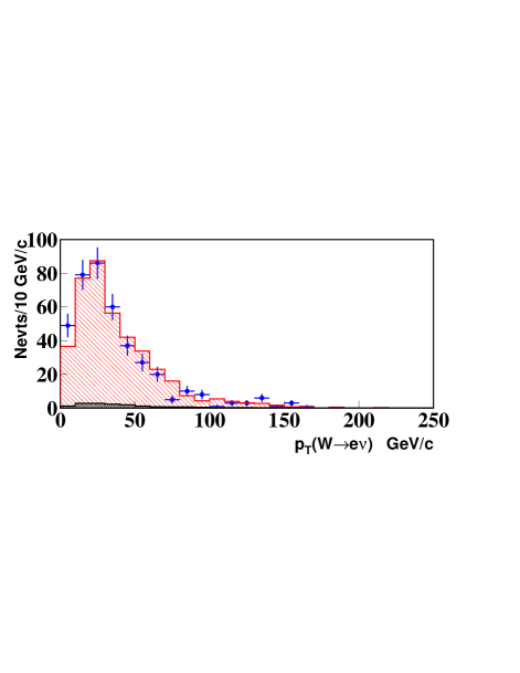
FIG. 11.: The $p_{T}$ distributions of the $e\nu$ system from the 1993–1995 (Run 1b) data. The solid circles are data. The light-shaded histogram is the SM prediction for the background, including the dark-shaded histogram, which represents the SM prediction for $WW/WZ$ processes.

Of the 399 events that satisfy the selection criteria, 18 events have $p_{T}(e\nu)>100$ GeV/$c$. The numbers of background and SM events in this $p_{T}$ range are estimated as $18.5\pm 1.8$ and $3.2\pm 0.5$, respectively. The absence of an excess of events with high $p_{T}(e\nu)$ excludes large deviations from SM couplings.

A Limits on Anomalous Couplings Using Minimum $p_{T}^{W}$

The $WW/WZ$ production cross section increases, especially at high $p_{T}^{W}$, as the coupling parameters deviate from the SM values, as shown in Fig. 2. The $p_{T}^{W}$ distribution for background is softer than that of $WW/WZ$ production with anomalous couplings. When events are selected with $p_{T}^{W}$ above some large minimum value, almost all background events are rejected, but a good fraction of signal with anomalous couplings remains, providing better sensitivity to such couplings. This kind of selection eliminates most of SM production, and therefore does not have sensitivity to the SM couplings. Moreover the 95% C.L. upper limit on the number of signal events ($N^{95\%{\rm C.L.}}$) can be obtained from the observed number of candidate events and the expected background beyond some minimum $p_{T}^{W}$ cutoff, using the method described in the report by the Particle Data Group [5]. To do this, Monte Carlo events are generated for pairs of anomalous couplings in grid points of $\Delta\kappa$ and $\lambda$. We assume that the couplings for $WW\gamma$ and $WWZ$ are equal. The expected number of events for each pair of anomalous couplings is calculated using the integrated luminosity of the data sample, and entered into a two-dimensional density plot with $\Delta\kappa$ and $\lambda$ as coordinate axes. The results are fitted with a two-dimensional parabolic function, and limits on anomalous couplings are calculated at the 95% C.L. from the intersection of the two-dimensional parabolic surface for the predicted number of events with a plane of $N^{95\%{\rm C.L.}}$ values. The resulting contour of constant probability is an ellipse in the $\Delta\kappa-\lambda$ plane. The numerical values for the “one-dimensional” 95% C.L. limits (setting one of the coordinates to zero) are summarized in Table V for different minimum values of $p_{T}^{W}$.

TABLE V.: Limits on $\lambda$ and $\Delta\kappa$ at the 95% C.L. as a function of minimum $p_{T}^{W}$, for $\Lambda$ = 1.5 TeV. The number of candidates ($N_{\rm cand}$), background ($N_{\rm BG}$), and the SM $WW/WZ$ predictions ($N_{\rm SM}$) are also listed.

$p^{W}_{T}$ (GeV/$c$)	$N_{\rm cand}$	$N_{\rm BG}$	$N_{\rm SM}$	$\lambda$	$\Delta\kappa$
	events	events	events	$(\Delta\kappa=0)$	$(\lambda=0)$
150	4	2.8	1.9	$(-0.66,0.67)$	$(-0.96,1.08)$
160	1	2.1	1.8	$(-0.54,0.54)$	$(-0.79,0.89)$
170	0	1.5	0.9	$(-0.52,0.52)$	$(-0.76,0.86)$
180	0	1.2	0.2	$(-0.59,0.58)$	$(-0.87,0.96)$
190	0	0.7	0.1	$(-0.64,0.64)$	$(-0.96,1.05)$
200	0	0.3	0.1	$(-0.74,0.73)$	$(-1.13,1.20)$

B Limits on Anomalous Couplings from the $p^{W}_{T}$ Spectrum

The limits obtained for some cutoff minimum $p_{T}^{W}$ do not take into account information that is available in the full $p^{W}_{T}$ spectrum, and depend on the chosen minimum $p_{T}$ value as well as on the overall normalization factors for background and predictions for signal. An alternative way to proceed is to fit the shape of kinematical distributions that are sensitive to anomalous couplings. This usually provides tighter limits, since it uses all the information contained in the differential distributions, and it is also less sensitive to overall normalization factors.

As described in Sec. I, the differential distribution that is most sensitive to anomalous couplings is the $p_{T}^{W(Z)}$ distribution. Our analysis relies on the $p_{T}(W\rightarrow e\nu)$ spectrum rather than $p_{T}(W\rightarrow jj)$ or $p_{T}(Z\rightarrow jj)$ because the resolution on $p_{T}(e\nu)$ (12.5 GeV/$c$) is better than on $p_{T}(jj)$ (16.7 GeV/$c$). This is primarily due to the ambiguity in assigning jets to the $W(Z)$ boson.

The differential cross sections have been exploited by previous publications  [10, 11, 12, 14, 15, 16, 17, 19, 20] for extracting limits on trilinear gauge boson couplings. We use a modified fit to the binned $p_{T}^{W}$ distribution to obtain limits, with the modification consisting of adding an extra bin in $p^{W}_{T}$ with no observed events, thereby improving the sensitivity to anomalous couplings [34].

Based on the number of expected $WW/WZ\rightarrow e\nu jj$ events, we choose two 25 GeV/$c$ bins between 0 and 50 GeV/$c$, five 10 GeV/$c$ bins from 50 to 100 GeV/$c$, two 20 GeV/$c$ bins from 100 to 140 GeV/$c$, one 30 GeV/$c$ bin from 140 to 170 GeV/$c$, and a single bin from 170 GeV/$c$ to 500 GeV/$c$. The cross section for $p_{T}^{W}>500$ GeV/$c$ is negligible for any anomalous couplings allowed by unitarity. For each bin $i$ of $p^{W}_{T}$, the probability $P_{i}$ for observing $N_{i}$ events is given by the Poisson distribution:

$$P_{i}=\frac{(b_{i}+{\cal L}\epsilon_{i}\sigma_{i}(\lambda,\Delta\kappa))^{N_{i}}}{N_{i}!}e^{-(b_{i}+{\cal L}\epsilon_{i}\sigma_{i}(\lambda,\Delta\kappa))},$$

where ${\cal L}$ is the luminosity, and $b_{i}$, $\epsilon_{i}$, and and $\sigma_{i}$ are the expected background, the total detection efficiency, and the cross section, respectively, for bin $i$. Our fast Monte Carlo is used to calculate $\epsilon_{i}\sigma_{i}(\lambda,\Delta\kappa)$. The joint probability for all $p^{W}_{T}$ bins is the product of the individual probabilities $P_{i}$, $P=\prod^{N_{\rm bin}}_{i=1}P_{i}.$ Since the values ${\cal L}$, $b_{i}$, and $\epsilon_{i}$ are measured values with their respective uncertainties, we assign them Gaussian prior distributions of mean $\mu=1$ and standard deviation $\sigma_{x}$:

$$P^{\prime}=\int{\cal{G}}_{f_{n}}df_{n}\int{\cal{G}}_{f_{b}}df_{b}\prod^{N_{\rm bin}}_{i=1}\frac{e^{f_{n}n_{i}+f_{b}b_{i}}(f_{n}n_{i}+f_{b}b_{i})^{N_{i}}}{N_{i}!},$$

where $n_{i}={\cal L}\epsilon_{i}\sigma_{i}$ is the predicted number of signal events, and ${\cal{G}}_{f_{n}}$ and ${\cal{G}}_{f_{b}}$ are Gaussian distributions for the fractions of signal and background events. The integrals are calculated using 50 evenly spaced points between $\pm 3$ standard deviations. For convenience, the log of the likelihood $L=\log P^{\prime}$ is used in the fit and the set of couplings that best describes the data is given by the point in the $\lambda-\Delta\kappa$ plane that maximizes the likelihood given in the above equation.

It is conventional to quote the limits on one coupling when all the others are set to their SM values. These “one-dimensional” limits at the 95% C.L., assuming that the $WW\gamma$ and $WWZ$ couplings are equal, are shown in Table VI. The limits are more stringent than those obtained using the minimum $p_{T}^{W}$ method.

TABLE VI.: Limits on anomalous trilinear gauge boson couplings at the 95% C.L. for three values of $\Lambda$ obtained using the fit to $p_{T}^{W}$ for data from the Run 1b.

Couplings	$\Lambda=1.0$ TeV	$\Lambda=1.5$ TeV	$\Lambda=2.0$ TeV
$\lambda_{\gamma}=\lambda_{Z}$ ($\Delta\kappa_{\gamma}=\Delta\kappa_{Z}=0$)	$-0.50,0.53$	$-0.42,0.45$	$-0.39,0.42$
$\Delta\kappa_{\gamma}=\Delta\kappa_{Z}$ ($\lambda_{\gamma}=\lambda_{Z}=0$)	$-0.66,0.90$	$-0.56,0.75$	$-0.52,0.70$
$\lambda_{\gamma}$ (HISZ) ($\Delta\kappa_{\gamma}=0$)	$-0.50,0.53$	$-0.42,0.45$	$-0.39,0.42$
$\Delta\kappa_{\gamma}$ (HISZ) ($\lambda_{\gamma}=0$)	$-0.78,1.15$	$-0.68,0.98$	$-0.63,0.91$
$\lambda_{\gamma}$ (SM $WWZ$) ($\Delta\kappa_{\gamma}=0$)	$-1.54,1.58$	$-1.53,1.56$
$\Delta\kappa_{\gamma}$ (SM $WWZ$) ($\lambda_{\gamma}=0$)	$-2.03,2.45$	$-1.79,2.12$
$\lambda_{Z}$ (SM $WW\gamma$) ($\Delta\kappa_{Z}=\Delta g^{Z}_{1}=0$)	$-0.58,0.62$	$-0.49,0.51$	$-0.45,0.48$
$\Delta\kappa_{Z}$ (SM $WW\gamma$) ($\lambda_{Z}=\Delta g^{Z}_{1}=0$)	$-0.86,1.12$	$-0.72,0.93$	$-0.67,0.87$

We have assumed thus far that the couplings $\Delta\kappa$ and $\lambda$ for $WWZ$ and $WW\gamma$ are equal. However, this is not the only possibility. Another common assumption leads to the HISZ relations [35]. These relations specify $\lambda_{Z}$, $\kappa_{Z}$, and $g_{1}^{Z}$ in terms of the independent variables $\lambda_{\gamma}$ and $\kappa_{\gamma}$, thereby reducing the number of independent couplings from five to two: $\Delta\kappa_{Z}=\frac{1}{2}\Delta\kappa_{\gamma}(1-\tan^{2}\theta_{W})$, $\Delta g_{1}^{Z}=\frac{1}{2}\Delta\kappa_{\gamma}/\cos^{2}\theta_{W}$, and $\lambda_{Z}=\lambda_{\gamma}$. These one-dimensional limits at the 95% C.L. are also shown in Table VI.

Since the $WWZ$ and $WW\gamma$ couplings are independent, it is interesting to find the limits on one when the other is set to its SM values. Table VI includes the one-dimensional limits at the 95% C.L. for both assumptions: limits on $\Delta\kappa_{\gamma}$ and $\lambda_{\gamma}$ when the $WWZ$ couplings are assumed to be standard, and limits on $\Delta\kappa_{Z}$ and $\lambda_{Z}$ when the $WW\gamma$ couplings are assumed to be standard. These results indicate that our analysis is more sensitive to $WWZ$ couplings, as should be expected from the larger overall SM couplings for $WWZ$ than for $WW\gamma$, and that our analysis is complementary to studies of the $W\gamma$ production process which is sensitive only to the $WW\gamma$ couplings.

C Combined Results for Run 1 on $WW/WZ\rightarrow e\nu jj$

The limits on anomalous couplings presented in this paper are significantly tighter than those in our previous publications [12, 16]. The primary reason for this is the increase in the amount of data (about a factor of six). We can obtain even stronger limits by combining the results from Run 1a and 1b. The analysis based on the Run 1a data is described in Refs [12, 16]. A summary of the signal and backgrounds for the two analyses [19] is given in Table IV.

The two analyses can be treated as different experiments. However, because both experiments used the same detector, there are certain correlated uncertainties, such as the uncertainties on the luminosity, lepton reconstruction and identification, and the theoretical prediction. Also, the background estimate is common to each experiment. The uncertainty on the $W/Z\rightarrow jj$ selection efficiency is assumed to be uncorrelated, since we use different cone sizes for jet reconstruction in the two analyses. (This hypothesis does not affect the results in any significant way.) The uncertainties for both analyses are summarized in Tables VII and VIII. Each uncertainty is weighted by the integrated luminosity for the respective data sample. Figure 12 shows the combined $p_{T}^{W}$ spectrum.

TABLE VII.: Common systematic uncertainties for Run 1a and Run 1b analyses.

Source of Uncertainty
Luminosity	5.4%
QCD corrections	14%
Electron and trigger efficiency	1.2%
Statistics of fast MC	1%
$\hbox to0.0pt{\kern 2.5pt/\hss}E_{T}$ smearing	5.1%
Jet energy scale	3.4%
Total	16%

TABLE VIII.: Uncorrelated systematic uncertainties for Run 1a and Run 1b analyses.

Source of Uncertainty	Run 1a	Run 1b
isajet vs pythia	9%	4%
Stat. uncertainties of $\epsilon(W\rightarrow jj)$	4%	2%
Parametrization of $\epsilon_{i}\sigma_{i}(\lambda,\Delta\kappa)$	4%	5%
Total (added in quadrature)	11%	7%
Background	13%	7%

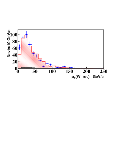
FIG. 12.: The $p_{T}^{W}$ spectrum for $e\nu jj$ candidates for the full Run 1 data sample. The solid circles are data. The light-shaded histogram is the sum of predictions from the SM and background, and the dark-shaded histogram is the SM prediction for $WW/WZ$ processes alone.

To set limits on anomalous couplings, we combine the results of the two analyses by calculating a combined likelihood function. The individual uncertainties on signal and background for each analysis are taken into account as in the previous section. Common systematic uncertainties are taken into account by introducing a common Gaussian prior distribution for the two data samples.

Combining results from Run 1a and Run 1b yields the 95% C.L. contours of constant probability shown in Fig. 13. The one and two dimensional 95% C.L. contour limits (corresponding to log-likelihood values of 1.92 and 3.00 units below the maximum, respectively) are shown as the inner contours, along with the unitarity limits from the $S$-matrix, shown as the outermost contours. Figure 13(a) shows the contour limits when couplings for $WW\gamma$ are assumed to be equal to those for $WWZ$. Figure 13(b) shows contour limits assuming the HISZ relations. In Figs. 13(c) and 13(d), SM $WW\gamma$ couplings are assumed and the limits are shown for $WWZ$ couplings. Assuming SM $WW\gamma$ couplings, the U(1) point that corresponds to the condition in which there is no $WWZ$ couplings ($\kappa_{Z}=0$, $\lambda_{Z}=0$, $g_{1}^{Z}=0$) is excluded at the 99% C.L. This is direct evidence for the existence of $WWZ$ couplings. These limits are slightly stronger than those from the 1993–1995 data alone. The one-dimensional 95% C.L. limits for four assumptions on the relation between $WW\gamma$ and $WWZ$ couplings: (i) $\Delta\kappa\equiv\Delta\kappa_{\gamma}=\Delta\kappa_{Z}$, $\lambda\equiv\lambda_{\gamma}=\lambda_{Z}$, (ii) HISZ relations, (iii) SM $WW\gamma$ couplings, and (iv) SM $WWZ$ couplings are listed in Table IX.

TABLE IX.: Limits on anomalous trilinear gauge boson couplings at 95% C.L. from the combined Run 1a and Run 1b data samples for these values of $\Lambda$.

Couplings	$\Lambda=1.0$ TeV	$\Lambda=1.5$ TeV	$\Lambda=2.0$ TeV
$\lambda_{\gamma}=\lambda_{Z}$ ($\Delta\kappa_{\gamma}=\Delta\kappa_{Z}=0$)	$-0.42,0.45$	$-0.36,0.39$	$-0.34,0.36$
$\Delta\kappa_{\gamma}=\Delta\kappa_{Z}$ ($\lambda_{\gamma}=\lambda_{Z}=0$)	$-0.55,0.79$	$-0.47,0.63$	$-0.43,0.59$
$\lambda_{\gamma}$ (HISZ) ($\Delta\kappa_{\gamma}=0$)	$-0.42,0.45$	$-0.36,0.39$	$-0.34,0.36$
$\Delta\kappa_{\gamma}$ (HISZ) ($\lambda_{\gamma}=0$)	$-0.69,1.04$	$-0.56,0.85$	$-0.53,0.78$
$\lambda_{\gamma}$ (SM $WWZ$) ($\Delta\kappa_{\gamma}=0$)	$-1.28,1.33$	$-1.21,1.25$
$\Delta\kappa_{\gamma}$ (SM $WWZ$) ($\lambda_{\gamma}=0$)	$-1.60,2.03$	$-1.38,1.70$
$\lambda_{Z}$ (SM $WW\gamma$) ($\Delta\kappa_{Z}=\Delta g_{1}^{Z}=0$)	$-0.47,0.51$	$-0.40,0.43$	$-0.37,0.40$
$\Delta\kappa_{Z}$ (SM $WW\gamma$) ($\lambda_{Z}=\Delta g_{1}^{Z}=0$)	$-0.74,0.99$	$-0.60,0.79$	$-0.54,0.72$
$\Delta g_{1}^{Z}$ (SM $WW\gamma$) ($\lambda_{Z}=\Delta\kappa_{Z}=0$)	$-0.75,1.06$	$-0.64,0.89$	$-0.60,0.81$

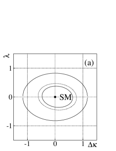
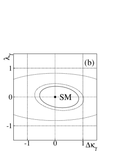
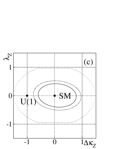
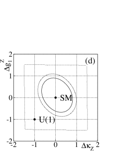
FIG. 13.: Contour limits on anomalous couplings at the 95% C.L. (two inner curves) and unitary constraints (outermost curves), assuming (a) $\Delta\kappa\equiv\Delta\kappa_{\gamma}=\Delta\kappa_{Z},\lambda\equiv\lambda_{\gamma}=\lambda_{Z}$; (b) HISZ relations; (c) and (d) SM $WW\gamma$ couplings. $\Lambda=1.5$ TeV is used for all four cases. The U(1) point is the expectation with no $WWZ$ couplings.

X Conclusions

We have searched for anomalous $WW$ and $WZ$ production in the $e\nu jj$ decay mode at $\sqrt{s}=1.8$ TeV. In a total of 82.3 pb^-1 of data from the 1993–1995 collider run at Fermilab, we observe 399 candidate events with an expected background of 387.5$\pm$38.1 events. The expected number of events from SM $WW/WZ$ production is $17.5\pm 3.0$ events for this integrated luminosity. The sum of the SM prediction and the background estimates is consistent with the observed number of events, indicating that no new physics phenomena is seen. Comparing the $p_{T}^{W}$ distributions of the observed events with theoretical predictions, we set limits on the $WW\gamma$ and $WWZ$ anomalous couplings. The limits on anomalous couplings are significantly tighter than those using the 1992–1993 data sample. The two results are combined to set even tighter limits on the anomalous couplings. With an assumption that the $WW\gamma$ and $WWZ$ couplings are equal, we obtain $-0.34<\lambda<0.36$ (with $\Delta\kappa=0$) and $-0.43<\Delta\kappa<0.59$ (with $\lambda=0$) at the 95% C.L. for a form factor scale $\Lambda=2.0$ TeV [36].

XI Acknowledgements

We thank the Fermilab and collaborating institution staffs for contributions to this work, and acknowledge support from the Department of Energy and National Science Foundation (USA), Commissariat à L’Energie Atomique (France), Ministry for Science and Technology and Ministry for Atomic Energy (Russia), CAPES and CNPq (Brazil), Departments of Atomic Energy and Science and Education (India), Colciencias (Colombia), CONACyT (Mexico), Ministry of Education and KOSEF (Korea), CONICET and UBACyT (Argentina), A.P. Sloan Foundation, and the Humboldt Foundation.

REFERENCES

- [1]
- [2] U. Baur and E. L. Berger, Phys Rev. D 41, 1476 (1990).
- [3] K. Hagiwara, J. Woodside and D. Zeppenfeld, Phys Rev. D 41, 2113 (1990).
- [4] J. Ellison and J. Wudka, UCR-D0-98-01, 1998, hep-ph/9804322 (unpublished).
- [5] Particle Data Group, Eur. Phys. J. C 3, 1 (1998).
- [6] K. Hagiwara, R.D. Peccei, D. Zeppenfeld and K. Hikasa, Nucl. Phys. B282, 253 (1987).
- [7] F. Boudjema et al., Phys. Rev. D 43, 2223 (1991).
- [8] U. Baur and D. Zeppenfeld, Phys. Lett. B 201, 383 (1988).
- [9] J. Alitti et al. (UA2 Collaboration), Phys. Lett. B 277, 194 (1992).
- [10] F. Abe et al. (CDF Collaboration), Phys. Rev. Lett. 74, 1936 (1995).
- [11] S. Abachi et al. (DØ Collaboration), Phys. Rev. Lett. 75, 1034 (1995); ibid., 78, 3634 (1997).
- [12] S. Abachi et al. (DØ Collaboration), Phys. Rev. D 56, 6742 (1997)
- [13] F. Abe et al. (CDF Collaboration), Phys. Rev. Lett. 78, 4536 (1997).
- [14] S. Abachi et al. (DØ Collaboration), Phys. Rev. Lett. 75, 1023 (1995); B. Abbott et al. (DØ Collaboration), Phys. Rev. D 58, 051101 (1998).
- [15] F. Abe et al. (CDF Collaboration), Phys. Rev. Lett. 75, 1017 (1995).
- [16] S. Abachi et al. (DØ Collaboration), Phys. Rev. Lett. 77, 3303 (1996).
- [17] B. Abbott et al. (DØ Collaboration), Phys. Rev. D, 60, 072002 (1999)
- [18] P. Abreu et al. (DELPHI Collaboration), Phys. Lett. B 459, 382 (1999); G. Abbiendi et al. (OPAL Collaboration), Eur. Phys. J. C 8, 191 (1999); M. Acciarri et al. (L3 Collaboration), Phys. Lett. B 467, 171 (1999); B. Barate et al. (ALEPH Collaboration), CERN-EP-98-178, 1998, submitted to Phys. Lett. B.
- [19] B. Abbott et al. (DØ Collaboration), Phys. Rev. Lett. 79, 1441 (1997).
-
[20]
A. Sánchez-Hernández, Ph.D.
Dissertation, CINVESTAV,
Mexico City, Mexico (1997),
http://www-d0.fnal.gov/results/publications_talks/thesis/thesis.html, unpublished. - [21] S. Abachi et al. (DØ Collaboration), Nucl. Instrum. Methods in Phys. Res. A 338, 185 (1994).
- [22] S. Abachi et al. (DØ Collaboration), Phys. Rev. Lett. 77, 3309 (1996); B. Abbott et al. (DØ Collaboration), Phys. Rev. Lett. 80, 3008 (1998); Phys. Rev. D 58, 12002 (1998); ibid., 58, 092003 (1998); B. Abbott et al. (DØ Collaboration), FERMILAB-Pub-99/237-E, hep-ex/9908057 (submitted to Phys. Rev. D); B. Abbott et al. (DØ Collaboration), Phys. Rev. Lett. 84, 222 (2000).
- [23] DØ Collaboration, R. Kehoe, in Proceedings of the Sixth International Conference on Calorimetry in High Energy Physics, Frascati, Italy (World Scientific, River Edge, NJ, 1996), FERMILAB-Conf-96/284-E.
- [24] S. Abachi et al. (DØ Collaboration), Phys. Rev. D 52, 4877 (1995).
- [25] J. Bantly et al., FERMILAB-TM-1995 (unpublished). To facilitate combination with previously published results, this analysis uses the older DØ luminosity of Ref. [19]. The recently updated 3.2% increase in luminosity, B. Abbott et al. (DØ Collaboration), hep-ex/990625, Sec. VII, pp. 21–22 (submitted to Phys. Rev. D), has little impact on these results.
-
[26]
M. L. Kelly, Ph.D. Thesis, Notre Dame (1996),
http://www-d0.fnal.gov/results/publications_talks/thesis/thesis.html, unpublished. - [27] F. Paige and S. Protopopescu, BNL Report BNL38034 (1986), unpublished. We used version 7.22.
- [28] T. Sjöstrand, Comput. Phys. Commun. 82, 74 (1994).
- [29] H. L. Lai et al. Phys. Rev. D 51, 4763 (1995).
- [30] J. Ohnemus, Phys. Rev. D 44, 1403 (1991); ibid., 44, 3477 (1991).
- [31] F.A. Berends et al., Nucl. Phys. B357, 32 (1991). We used version 3.0.
- [32] G. Marchesini et al., Comput. Phys. Commun. 67, 465 (1992). We used version 5.7.
- [33] B. Abbott et al. (DØ Collaboration), Phys. Rev. Lett. 79, 1203 (1997).
-
[34]
G. L. Landsberg, Ph.D. Thesis, State University of
New York at Stony Brook (1994),
http://www-d0.fnal.gov/results/publications_talks/thesis/thesis.html, unpublished. - [35] K. Hagiwara, S. Ishihara, R. Szalapski and D. Zeppenfeld, Phys. Rev. D 48, 2182 (1993); Phys. Lett. B 283, 353 (1992). They parametrize the couplings in terms of the couplings: , and .
- [36] Subsequent to the publication of Ref. [19] which summarized this analysis, these results were combined with the other DØ measurements of anomalous and couplings, using the method described in B. Abbott et al. (DØ Collaboration), Phys. Rev. D 58 31102 (1998), to provide the experiment’s most restrictive limits which were reported in Ref. [17].