Abstract

This work is devoted to the experimental study of the longitudinal hadronic shower development in the ATLAS barrel combined prototype calorimeter consisting of the lead-liquid argon electromagnetic part and the iron-scintillator hadronic part. The results have been obtained on the basis of the 1996 combined test beam data which have been taken on the H8 beam of the CERN SPS, with the pion beams of 10, 20, 40, 50, 80, 100, 150 and 300 GeV/c. The degree of description of generally accepted Bock parameterization of the longitudinal shower development has been investigated. It is shown that this parameterization does not give satisfactory description for this combined calorimeter. Some modification of this parameterization, in which the $e/h$ ratios of the compartments of the combined calorimeter are used, is suggested and compared with the experimental data. The agreement between such parameterization and the experimental data is demonstrated.

1 Introduction

One of the important questions of hadron calorimetry is the question of the longitudinal development of hadronic showers. This question is especially important for a combined calorimeter. This work is devoted to the study of the longitudinal hadronic shower development in the ATLAS barrel combined prototype calorimeter [1, 2, 3, 4, 5].

This work has been performed on the basis of the 1996 combined test beam data [5]. Data were taken on the H8 beam of the CERN SPS with the pion beams of 10, 20, 40, 50, 80, 100, 150 and 300 GeV/c.

2 Combined Calorimeter

The future ATLAS experiment [1] will include in the central (“barrel”) region a calorimeter system composed of two separate units: the liquid argon electromagnetic calorimeter (LAr) [3] and the tile iron-scintillating hadronic calorimeter (Tile) [2]. For detailed understanding of performance of the future ATLAS combined calorimeter the combined calorimeter prototype setup has been made consisting of the LAr electromagnetic calorimeter prototype inside the cryostat and downstream the Tile calorimeter prototype as shown in Fig. 1.

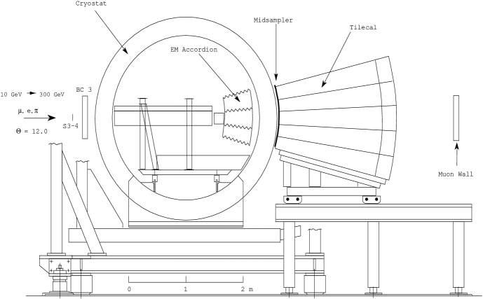
Figure 1: Test beam setup for the combined LAr and Tile calorimeters run.

The dead material upstream of the LAr calorimeter was about $0.1\ \lambda_{\pi}$ and the one between the two calorimeters was about $0.3\ \lambda_{\pi}$. The two calorimeters have been placed with their central axes at an angle to the beam of $12^{\circ}$. At this angle the two calorimeters have an active thickness of $8.6\ \lambda_{\pi}$. Between the active part of the LAr and the Tile detectors a layer of scintillator was installed, called the midsampler. The midsampler consists of five scintillators, $20\times 100$ cm² each, fastened directly to the front face of the Tile modules. The scintillator is 1 cm thick. Beam quality and geometry were monitored with a set of beam wire chambers BC1, BC2, BC3 and trigger hodoscopes placed upstream of the LAr cryostat. To detect punchthrough particles and to measure the effect of longitudinal leakage a “muon wall” consisting of 10 scintillator counters (each 2 cm thick) was located behind the calorimeters at a distance of about 1 metre.

2.1 Electromagnetic Calorimeter

The electromagnetic LAr calorimeter prototype consists of a stack of three azimuthal modules, each one spanning $9^{\circ}$ in azimuth and extending over 2 m along the Z direction. The calorimeter structure is defined by 2.2 mm thick steel-plated lead absorbers, folded to an accordion shape and separated by 3.8 mm gaps, filled with liquid argon. The signals are collected by Kapton electrodes located in the gaps. The calorimeter extends from an inner radius of 131.5 cm to an outer radius of 182.6 cm, representing (at $\eta=0$) a total of 25 radiation lengths ($X_{0}$), or 1.22 interaction lengths ($\lambda_{I}$) for protons. The calorimeter is longitudinally segmented into three compartments of $9\ X_{0}$, $9\ X_{0}$ and $7\ X_{0}$, respectively. More details about this prototype can be found in [1, 6]. In front of the EM calorimeter a presampler was mounted. The active depth of liquid argon in the presampler is 10 mm and the strip spacing is 3.9 mm. The cryostat has a cylindrical form with 2 m internal diameter, filled with liquid argon, and is made out of a 8 mm thick inner stainless-steel vessel, isolated by 30 cm of low-density foam (Rohacell), itself protected by a 1.2 mm thick aluminum outer wall.

2.2 Hadronic Calorimeter

The hadronic Tile calorimeter is a sampling device using steel as the absorber and scintillating tiles as the active material [2]. The innovative feature of the design is the orientation of the tiles which are placed in planes perpendicular to the Z direction [7]. For a better sampling homogeneity the 3 mm thick scintillators are staggered in the radial direction. The tiles are separated along Z by 14 mm of steel, giving a steel/scintillator volume ratio of 4.7. Wavelength shifting fibers (WLS) running radially collect light from the tiles at both of their open edges. The hadron calorimeter prototype consists of an azimuthal stack of five modules. Each module covers $2\pi/64$ in azimuth and extends 1 m along the Z direction, such that the front face covers $100\times 20$ cm². Read-out cells are defined by grouping together a bundle of fibers into one photomultiplier (PMT). Each of the 100 cells is read out by two PMTs with $\Delta\phi=2\pi/64\approx 0.1$, while the segmentation along the Z axis is made by grouping fibers into read-out cells spanning $\Delta Z=20$ cm ($\Delta\eta\approx 0.1$). Each module is read out in four longitudinal segments (corresponding to about 1.5, 2, 2.5 and 3 $\lambda_{I}$ at $\eta=0$). More details of this prototype can be found in [1, 8].

3 Event Selection

We applied some cuts similar to [5] to eliminate the nonsingle track pion events, the beam halo, the events with an interaction before LAr calorimeter and muon events. The set of cuts applied is the following:

• single-track pion events were selected off-line by requiring the pulse height of the beam scintillation counters and the energy released in the presampler of the electromagnetic calorimeter to be compatible with that of a single particle;

• beam halo events were removed with appropriate cuts on the horizontal and vertical positions of the incoming track impact point and the space angle with respect to the beam axis as measured with the two beam chambers;

• a cut on the total energy rejects incoming muon.

4 Energy Reconstruction

To reconstruct the hadron energy in longitudinal segments the $e/h$ method of the energy reconstruction, suggested in [9], has been used. In this method the energy of hadrons in a combined calorimeter is determined by the following formula:

$$E=c_{LAr}\cdot(e/\pi)_{LAr}\cdot R_{LAr}+c_{Tile}\cdot(e/\pi)_{Tile}\cdot R_{Tile}+E_{dm}\ ,$$ (1)

Here $R_{LAr}$ ($R_{Tile}$) is the LAr (Tile) calorimeter response, $c_{LAr}=1/e_{LAr}$, $c_{Tile}=1/e_{Tile}$, $e_{LAr}$ and $e_{Tile}$ are the electron calibration constants for LAr and Tile calorimeters, $e/\pi$ ratios are equal to

$$\Bigl{(}\frac{e}{\pi}\Bigr{)}_{LAr}=\frac{(e/h)_{LAr}}{1+((e/h)_{LAr}-1)f_{\pi^{0},LAr}}\ .$$ (2)

$$\Bigl{(}\frac{e}{\pi}\Bigr{)}_{Tile}=\frac{(e/h)_{Tile}}{1+((e/h)_{Tile}-1)f_{\pi^{0},Tile}}\ .$$ (3)

This method uses only the known $e/h$ ratios and the electron calibration constants and does not require the previous determination of any parameters by a minimization technique. The value of the $(e/h)_{LAr}$ ratio of the electromagnetic compartment has been obtained in [10] and equal to $(e/h)_{LAr}=1.77\pm 0.02$. This value agrees with with estimation of $>1.7$ obtained in [11].

For Tile calorimeter the value of $(e/h)_{Tile}=1.30\pm 0.04$ is used [12, 13].

The fraction of the shower energy going into the electromagnetic channel for LAr compartment is

$$f_{\pi^{0},LAr}=0.11\cdot ln{(E_{beam})}\ .$$ (4)

The electromagnetic fraction in the Tile calorimeter, which samples the final part of shower, is equal to the one for shower with energy $E_{Tile}$:

$$f_{\pi^{0},Tile}=0.11\cdot ln{(E_{Tile})}\ ,$$ (5)

where

$$E_{Tile}=c_{Tile}\cdot(e/\pi)_{Tile}\cdot R_{Tile}\ .$$ (6)

Special attention has been devoted to understanding of the energy loss in the dead material placed between the active part of the LAr and the Tile detectors. The term $E_{dm}$ accounts for this. This term is taken to be proportional to the geometrical mean of the energy released in the last electromagnetic compartment ($E_{LAr,3}$) and the first hadronic compartment ($E_{Tile,1}$)

$$E_{dm}=c_{dm}\cdot\sqrt{E_{LAr,3}\cdot E_{Tile,1}}$$ (7)

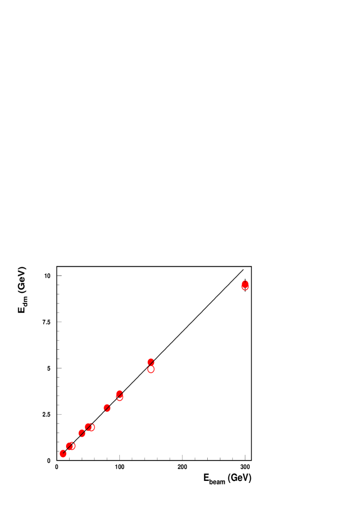
Figure 2: The comparison between the Monte Carlo simulation (open circles) and the calculated values (solid circles).

similar to [5]. We used the value of $c_{dm}=0.31$. This value has been obtained on the basis of the results of the Monte Carlo simulation [14]. These Monte Carlo (Fluka) results (open circles) are shown in Fig. 2 together with the values (solid circles) obtained by using the expression (7). The good agreement is observed. Also the linear behaviour as a function of the beam energy is demonstrated. The mean energy loss is equal to about $3.7\pm 0.4\%$ (spread).

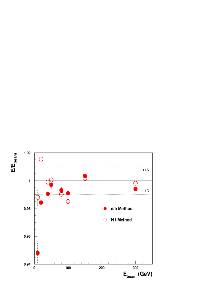
Figure 3: The demonstration of the correctness of the reconstruction of the mean values of energies by the $e/h$ method (black circles): the energy linearity, $E_{rec}/E_{beam}$ as a function of the beam energy. It is also shown the same for the cells weighting $H1$ method (open circles).

The $e/h$ method [9] has been tested on the basis of the 1996 test beam data of the ATLAS combined prototype calorimeter and demonstrated the correctness of the reconstruction of the mean values of energies as shown in Fig. 3. As can be seen the deviation from linearity for the $e/h$ method is about $1\%$.

We used this energy reconstruction method and obtained the energy depositions, $E_{i}$, in each longitudinal sampling with the thickness of $\Delta x_{i}$ in units $\lambda_{\pi}$. We transformed these depositions into the differential energy depositions using the formula:

$$(\Delta E/\Delta x)_{i}=E_{i}/\Delta x_{i}\ .$$ (8)

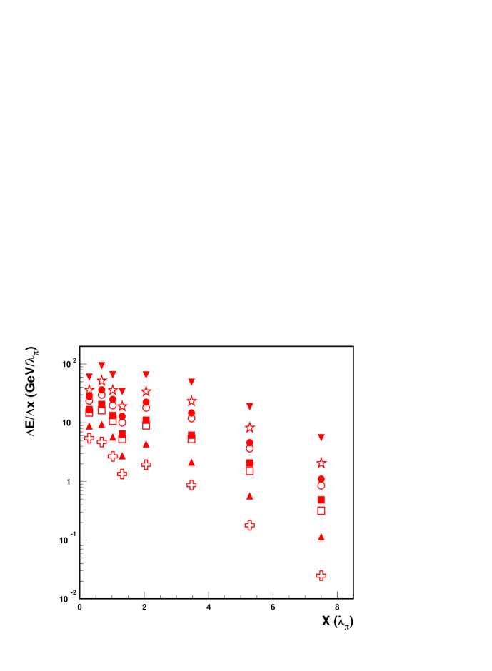
Figure 4: The differential longitudinal energy depositions in each longitudinal sampling for 10 GeV (crosses), 20 GeV (black top triangles), 40 GeV (open squares), 50 GeV (black squares), 80 GeV (open circles), 100 GeV (black circles), 150 GeV (stars) and 300 GeV (black bottom triangles) energies as a function of the longitudinal coordinate $x$ in units $\lambda_{\pi}$ for combined calorimeter.

Table 1 and Fig. 4 show the differential energy depositions as a function of the longitudinal coordinate $x$ for 10 GeV (crosses), 20 GeV (black top triangles), 40 GeV (open squares), 50 GeV (black squares), 80 GeV (open circles), 100 GeV (black circles), 150 GeV (stars), 300 GeV (black bottom triangles) energies. Some interesting special features are observed: the maximum in the region of the LAr calorimeter, then the local minimum in the point corresponding to the energy losses in the dead material, then the local maximum again.

5 Longitudinal Shower Development

The next important question is understanding and description of these experimental data.

There is the well known parameterization of the longitudinal hadronic shower development from the shower origin suggested in [15]

$$\frac{dE_{s}(x)}{dx}=N\ \Biggl{\{}w\ \biggl{(}\frac{x}{X_{0}}\biggr{)}^{a-1}\ e^{-b\frac{x}{X_{0}}}\ +\ (1-w)\ \biggl{(}\frac{x}{\lambda_{I}}\biggr{)}^{a-1}\ e^{-d\frac{x}{\lambda_{I}}}\Biggr{\}}\ ,$$ (9)

where $X_{0}$ is the radiation length, $\lambda_{I}$ is the interaction length, $a,\ b,\ d,\ w$ are parameters, $N$ is the normalization factor, $a=0.6165+0.3193\ lnE$, $b=0.2198$, $d=0.9099-0.0237\ lnE$, $\omega=0.4634$.

This parameterization is from the shower origin. But our data are from the calorimeter face and due to the unsufficient longitudinal segmentation can not be transformed to the shower origin. Therefore, we used the analytical representation of the hadronic shower longitudinal development from the calorimeter face [16]. This representation is a result of the integration of the longitudinal profile from the shower origin over the shower position:

$$\frac{dE(x)}{dx}=\int\limits_{0}^{x}\frac{dE_{s}(x-x_{v})}{dx}\ e^{-\frac{x_{v}}{\lambda_{I}}}\ dx_{v}\ ,$$ (10)

where $x_{v}$ is a coordinate of the shower vertex. This representation has the following form:

$$\frac{dE(x)}{dx} = N\ \Biggl{\{}\frac{wX_{0}}{a}\biggl{(}\frac{x}{X_{0}}\biggr{)}^{a}e^{-b\frac{x}{X_{0}}}{}_{1}F_{1}\biggl{(}1,a+1,\biggl{(}b-\frac{X_{0}}{\lambda_{I}}\biggr{)}\frac{x}{X_{0}}\biggr{)}$$ (11)

$$+\ \frac{(1-w)\lambda_{I}}{a}\biggl{(}\frac{x}{\lambda_{I}}\biggr{)}^{a}e^{-d\frac{x}{\lambda_{I}}}{}_{1}F_{1}\biggl{(}1,a+1,\bigl{(}d-1\bigr{)}\frac{x}{\lambda_{I}}\biggr{)}\Biggr{\}}.$$

Here ${}_{1}F_{1}(\alpha,\beta,z)$ is the confluent hypergeometric function and $N$ is the normalisation factor which equal to

$$N=\frac{E_{beam}}{\lambda_{I}\ \Gamma(a)\ \bigl{(}w\ X_{0}\ b^{-a}+(1-w)\ \lambda_{I}\ d^{-a}\bigr{)}}\ .$$ (12)

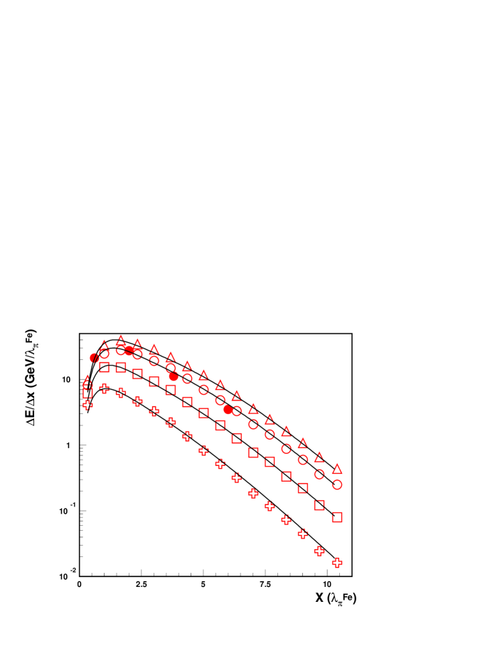
Figure 5: The demonstration of the correctness of the formula (11). The comparison between the calculations by this formula and the experimental data at 20 GeV (crosses), 50 GeV (squares), 100 GeV (open circles), 140 GeV (triangles) energies for conventional iron-scintillator calorimeter [17] and at 100 GeV (black circles) for the Tile calorimeter as a function of the longitudinal coordinate $x$ in units $\lambda_{\pi,Fe}$

Fig. 5 demonstrates the correctness of the above formula. The calculations by this formula are compared with the experimental data at 20 GeV (crosses), 50 GeV (squares), 100 GeV (open circles), 140 GeV (triangles) energies for conventional iron-scintillator calorimeter [17] and at 100 GeV (black circles) for the Tile calorimeter as a function of the longitudinal coordinate $x$ in units $\lambda_{\pi,Fe}$. The good agreement is observed. Note that formula (9) is given for a calorimeter characterizing by the certain $X_{0}$ and $\lambda_{I}$ values.

We have found in literature no algorithm for the hadronic shower development in a combined calorimeter. We suggest the following algorithm of combination of the LAr and Tile curves of the differential longitudinal energy deposition $dE/dx$ (Fig. 6). The first part of the combined curve is the beginning of the LAr curve, the second part is the Tile curve. At first a hadronic shower develops in the LAr calorimeter to the boundary value $x_{LAr}$. This value corresponds to certain integrated measured energy $E_{LAr}$. Then using the corresponding integrated Tile curve, $E(x)=\int_{0}^{x}(dE/dx)dx$, (Fig. 7) we find the point $x_{Tile}$ in which the energy is equal to $E_{Tile}(x_{Tile})=E_{LAr}+E_{dm}$. From this point a shower continues to develop in the Tile calorimeter. In principle, instead of the measured value of $E_{LAr}$ one can use the calculated value of $E_{LAr}=\int_{0}^{x_{LAr}}(dE/dx)dx$ obtained from the integrated LAr curve (Fig. 7).

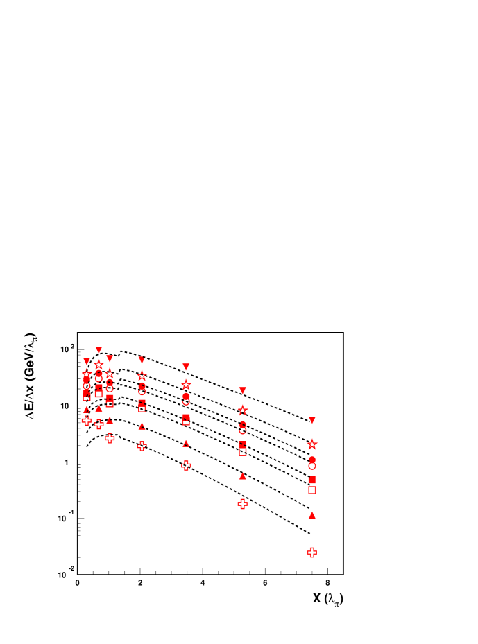
Figure 8: The comparison between the experimental differential energy depositions at 10 GeV (crosses), 20 GeV (black top triangles), 40 GeV (open squares), 50 GeV (black squares), 80 GeV (open circles), 100 GeV (black circles), 150 GeV (stars), 300 GeV (black bottom triangles) and the calculated curves as a function of the longitudinal coordinate $x$ in units $\lambda_{\pi}$.

In this way we obtained the combined curves. Fig. 8 shows a comparison between the experimental differential energy depositions at 10 GeV (crosses), 20 GeV (black top triangles), 40 GeV (open squares), 50 GeV (black squares), 80 GeV (open circles), 100 GeV (black circles), 150 GeV (stars), 300 GeV (black bottom triangles) as a function of the longitudinal coordinate $x$ in units $\lambda_{\pi}$. It can be seen that there is a significant disagreement between the experimental data and the combined curves in the region of the LAr calorimeter and especially at low energies.

We attempted to understand this disagreement. We considered the experimental database used by Bock et al. [15] for their parametrisation. It turns out that:

• The parameters given in [15] parameterization have been obtained by using the data from three iron-scintillator calorimeters and one lead-scintillator calorimeter:

  • CERN, WA1, $Fe$ (50 mm) + $Sc$ (6 mm), pions at 15, 50, 140 GeV, $e/h\approx 1.3$;

  • FNAL, 379, $Fe$ (38.4 – 51.2 mm) + $Sc$ (6.4 mm), pions at 375 and 400 GeV, $e/h\approx 1.3$;

  • CERN, the combined UA1 calorimeter, the electromagnetic part: $Pb$ (2 – 3 mm) + $Sc$ (1.5 – 2 mm), pions at 10, 20, 40, 60 GeV, $e/h\approx 1.1$ and the hadronic part: $Fe$ (50 mm) + $Sc$ (10 mm), $e/h\approx 1.3$.

  As to the used iron-scintillator calorimeters there is sufficient number of experimental points in our (10 – 300 GeV) beam energy range. At the same time the situation for the lead-scintillator calorimeter is quite different. There is a very limited number of points and the energy range of (10 – 60 GeV ) is essentially lower than used in our work.

• The $e/h$ ratio of the LAr calorimeter is $\approx 1.6$ times greater than their calorimeter.

• This parameterization does not include such essential feature of a calorimeter as the $e/h$ ratio.

We attempted to improve the description and tried several modifications and adjustments of some parameters of this parameterization. It turned out that the changes of two parameters $b$ and $w$ in the formula (11) in such a way $b_{Bock}=0.22$, $b_{new}=0.34=b_{Bock}\cdot(e/h)_{new}/(e/h)_{Bock}$, $w_{Bock}=0.4634$, $w_{new}=0.6\cdot K$, where $K$ factor is

$$K=\biggl{(}\frac{e}{\pi}\biggr{)}_{new}\biggr{/}\biggl{(}\frac{e}{\pi}\biggr{)}_{Bock}\ \ ,$$ (13)

$$\frac{e}{\pi}=\frac{e/h}{1+(e/h-1)f_{\pi^{0}}}$$ (14)

made it possible to obtain the reasonable description of the experimental data. This is shown in Fig. 9 in which the experimental differential longitudinal energy depositions at 10 GeV (crosses), 20 GeV (black top triangles), 40 GeV (open squares), 50 GeV (black squares), 80 GeV (open circles), 100 GeV (black circles), 150 GeV (stars), 300 GeV (black bottom triangles) energies as a function of the longitudinal coordinate $x$ in units $\lambda_{\pi}$ for the combined calorimeter and the results of the description by the modified parameterization are compared. There is a reasonable agreement (probability of description is more than $5\%$) between the experimental data and the curves taking into account uncertainties in the parametrization function [15]. In such case the Bock parameterization is the private case for some fixed the $e/h$ ratio.

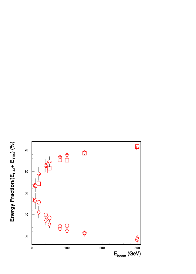
Figure 10: Energy deposition (percentage) in the LAr and Tile calorimeters at different beam energies. The circles (squares) are the measured energy depositions in the LAr (Tile) calorimeter, the diamonds (crosses) are the calculated energy depositions in the ones.

The obtained parameterization has some additional applications. For example, this formula may be used for an estimate of the energy deposition in various parts of a combined calorimeter. This demonstrates in Fig. 10 in which the measured and calculated relative values of the energy deposition in the LAr and Tile calorimeters are presented. The relative energy deposition in the LAr calorimeter decreases from about 50% at 10 $GeV$ to 30% at 300 $GeV$. On the contrary, the one in Tile calorimeter increases with the energy increasing.

6 Conclusions

The experimental longitudinal hadronic shower profiles in combined calorimeter consisting of the lead-argon electromagnetic part and iron-scintillator hadronic part have been obtained. The degree of description of the generally accepted Bock parameterization of the longitudinal shower development has been investigated. It is shown that this parameterization does not give satisfactory description for this combined calorimeter. Some modification of this parameterization, in which the $e/h$ ratios of the compartments of combined calorimeter are used, is suggested and compared with experiment. The agreement between such parameterization and the experimental data is demonstrated.

7 Acknowledgments

This work is the result of the efforts of many people from the ATLAS Collaboration. The authors are greatly indebted to all Collaboration for their test beam setup and data taking. Authors are grateful Peter Jenni and Marzio Nessi for fruitful discussion and support of this work. We are thankful Julian Budagov and Jemal Khubua for their attention and support of this work. We are also thankful Illias Efthymiopoulos and Irene Vichou for fruitful discussion.

Table 1: The differential energy depositions $\Delta E/\Delta x$ as a function of the longitudinal coordinate $x$ for the various beam energies.

N	x	$E_{beam}$ (GeV)
depth	($\lambda_{\pi}$)	10	20	40	50
1	0.294	$5.45\pm 0.08$	$8.58\pm 0.16$	$14.3\pm 0.2$	$16.6\pm 0.4$
2	0.681	$4.70\pm 0.08$	$9.10\pm 0.15$	$16.7\pm 0.2$	$20.8\pm 0.3$
3	1.026	$2.66\pm 0.06$	$5.55\pm 0.11$	$11.1\pm 0.2$	$13.6\pm 0.2$
dm	1.315	$1.35\pm 0.07$	$2.75\pm 0.14$	$5.28\pm 0.26$	$6.46\pm 0.32$
4	2.06	$1.93\pm 0.03$	$4.35\pm 0.06$	$8.99\pm 0.08$	$11.0\pm 0.1$
5	3.47	$0.87\pm 0.02$	$2.13\pm 0.04$	$5.29\pm 0.06$	$6.15\pm 0.10$
6	5.28	$0.18\pm 0.01$	$0.57\pm 0.02$	$1.50\pm 0.03$	$2.07\pm 0.05$
7	7.50	$0.025\pm 0.003$	$0.11\pm 0.01$	$0.32\pm 0.01$	$0.49\pm 0.02$
N	x	$E_{beam}$ (GeV)
depth	($\lambda_{\pi}$)	80	100	150	300
1	0.294	$22.6\pm 0.6$	$28.4\pm 0.6$	$36.3\pm 0.7$	$61.3\pm 1.5$
2	0.681	$30.4\pm 0.4$	$37.6\pm 0.5$	$53.5\pm 0.8$	$97.9\pm 1.7$
3	1.026	$20.3\pm 0.3$	$25.7\pm 0.4$	$37.2\pm 0.6$	$68.9\pm 1.2$
dm	1.315	$10.1\pm 0.5$	$12.8\pm 0.6$	$19.0\pm 1.0$	$34.1\pm 1.7$
4	2.06	$18.0\pm 0.1$	$22.4\pm 0.2$	$33.9\pm 0.3$	$64.8\pm 0.7$
5	3.47	$11.9\pm 0.1$	$14.6\pm 0.2$	$23.3\pm 0.2$	$49.0\pm 0.5$
6	5.28	$3.66\pm 0.06$	$4.57\pm 0.08$	$8.18\pm 0.13$	$18.6\pm 0.3$
7	7.50	$0.86\pm 0.03$	$1.10\pm 0.04$	$2.04\pm 0.06$	$5.54\pm 0.15$

.

Figure 6: The calculated differential longitudinal energy deposition, $dE/dx$, as a function of the longitudinal coordinate $x$ in units $\lambda_{\pi}$ for the LAr (top) and Tile (bottom) calorimeters at $20-300\ GeV$.

Figure 7: The integrated longitudinal energy depositions, $E(x)$ $=$ $\int dE/dxdx$, as a function of the longitudinal coordinate $x$ in units of $\lambda_{\pi}$ for the LAr (top) and Tile (bottom) calorimeters at 20 – 300 $GeV$.

Figure 9: The experimental differential longitudinal energy depositions at 10 GeV (crosses), 20 GeV (black top triangles), 40 GeV (open squares), 50 GeV (black squares), 80 GeV (open circles), 100 GeV (black circles), 150 GeV (stars), 300 GeV (black bottom triangles) energies as a function of the longitudinal coordinate $x$ in units $\lambda_{\pi}$ for the combined calorimeter and the results of the description by the modified parameterization.

References

- [1] ATLAS Collaboration, ATLAS Technical Proposal, CERN/LHCC/ 94-93, CERN, Geneva, Switzerland.
- [2] ATLAS Collaboration, ATLAS TILE Calorimeter TDR; CERN/ LHCC/96-42, ATLAS TDR 3, 1996, CERN, Geneva, Switzerland.
- [3] ATLAS Collaboration, ATLAS Liquid Argon Calorimeter Technical Design Report, CERN/LHCC/96-41, ATLAS TDR 2, 1996, CERN, Geneva, Switzerland.
- [4] Z. Ajaltouni et al., NIM A387 (1997) 335.
- [5] M. Cobal , ATL-TILECAL-98-168, 1998, CERN, Geneva, Switzerland.
- [6] D.M. Gingrich , (RD3 Collaboration), NIM A364 (1995) 290.
- [7] O. Gildemeister, F. Nessi-Tedaldi and M. Nessi, Proc. 2 Int. Conf. on Calorimetry in HEP, Capri, 1991.
- [8] F. Ariztizabal et al., NIM A349 (1994) 384.
- [9] Y.A. Kulchitsky , JINR-E1-99-317, JINR, Dubna, Russia; ATL-TILECAL-99-025, 1999, CERN, Geneva, Switzerland.
- [10] Y.A. Kulchitsky, M.V. Kuzmin, V.B. Vinogradov, JINR-E1-99-303, JINR, Dubna, Russia; ATLAS-TILECAL-99-021, 1999, CERN, Geneva, Switzerland.
- [11] R. Wigmans, Proc. 2 Int. Conf. on Calorimetry in HEP, Capri, 1991.
- [12] J.A. Budagov, Y.A. Kulchitsky, V.B. Vinogradov , JINR-E1-95-513, JINR, Dubna, Russia; ATL-TILECAL-95-72, 1995, CERN, Geneva, Switzerland.
- [13] Y.A. Kulchitsky, V.B. Vinogradov, JINR-E1-99-12, JINR, Dubna, Russia; ATL-TILECAL-99-002, 1999, CERN, Geneva, Switzerland.
- [14] I. Efthymiopoulos, Private communication.
- [15] R. Bock et al, NIM 186 (1981) 533.
- [16] Y.A. Kulchitsky, V.B. Vinogradov, NIM A413 (1998) 484.
- [17] E. Hughes, Proceedings of the 1 Int. Conf. on Calorimetry in HEP, p. 525, FNAL, Batavia, 1990.