Abstract

The new simple method of the energy reconstruction for a combined calorimeter, which we called the $e/h$ method, is suggested. It uses only the known $e/h$ ratios and the electron calibration constants and does not require the determination of any parameters by a minimization technique. The method has been tested on the basis of the 1996 test beam data of the ATLAS barrel combined calorimeter and demonstrated the correctness of the reconstruction of the mean values of energies. The obtained fractional energy resolution is $[(58\pm 3)\%/\sqrt{E}+(2.5\pm 0.3)\%]\oplus(1.7\pm 0.2)/E$. This algorithm can be used for the fast energy reconstruction in the first level trigger.

1 Introduction

The key question of calorimetry generally and hadronic calorimetry in particular is the energy reconstruction. This question is especially important when a hadronic calorimeter have a complex structure being a combined calorimeter. Such is the combined calorimeter of the ATLAS detector [1].

In this paper we describe the new simple method of the energy reconstruction for a combined calorimeter, which we called the $e/h$ method, and demonstrate its performance on the basis of the test beam data of the ATLAS combined prototype calorimeter.

2 Combine Calorimeter

The combined calorimeter prototype setup has been made consisting of the LAr electromagnetic calorimeter prototype inside the cryostat and downstream the Tile calorimeter prototype as shown in Fig. 1.

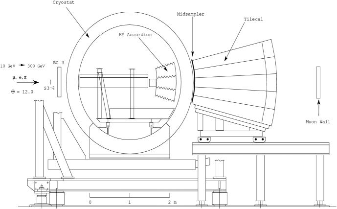
Figure 1: Test beam setup for the combined LAr and Tile calorimeters run.

The two calorimeters have been placed with their central axes at an angle to the beam of $12^{\circ}$. At this angle the two calorimeters have an active thickness of 10.3 $\lambda_{I}$. Beam quality and geometry were monitored with a set of beam wire chambers BC1, BC2, BC3 and trigger hodoscopes placed upstream of the LAr cryostat. To detect punchthrough particles and to measure the effect of longitudinal leakage a “muon wall” consisting of 10 scintillator counters (each 2 cm thick) was located behind the calorimeters at a distance of about 1 metre.

2.1 Electromagnetic Calorimeter

The electromagnetic LAr calorimeter prototype consists of a stack of three azimuthal modules, each one spanning $9^{\circ}$ in azimuth and extending over 2 m along the Z direction. The calorimeter structure is defined by 2.2 mm thick steel-plated lead absorbers, folded to an accordion shape and separated by 3.8 mm gaps, filled with liquid argon. The signals are collected by Kapton electrodes located in the gaps. The calorimeter extends from an inner radius of 131.5 cm to an outer radius of 182.6 cm, representing (at $\eta=0$) a total of 25 radiation lengths ($X_{0}$), or 1.22 interaction lengths ($\lambda_{I}$) for protons. The calorimeter is longitudinally segmented into three compartments of $9\ X_{0}$, $9\ X_{0}$ and $7\ X_{0}$, respectively. More details about this prototype can be found in [1, 2].

The cryostat has a cylindrical form with 2 m internal diameter, filled with liquid argon, and is made out of a 8 mm thick inner stainless-steel vessel, isolated by 30 cm of low-density foam (Rohacell), itself protected by a 1.2 mm thick aluminum outer wall.

2.2 Hadronic Calorimeter

The hadronic Tile calorimeter is a sampling device using steel as the absorber and scintillating tiles as the active material [3]. The innovative feature of the design is the orientation of the tiles which are placed in planes perpendicular to the Z direction [4]. For a better sampling homogeneity the 3 mm thick scintillators are staggered in the radial direction. The tiles are separated along Z by 14 mm of steel, giving a steel/scintillator volume ratio of 4.7. Wavelength shifting fibres (WLS) running radially collect light from the tiles at both of their open edges. The hadron calorimeter prototype consists of an azimuthal stack of five modules. Each module covers $2\pi/64$ in azimuth and extends 1 m along the Z direction, such that the front face covers $100\times 20$ cm². The radial depth, from an inner radius of 200 cm to an outer radius of 380 cm, accounts for 8.9 $\lambda$ at $\eta=0$  (80.5 $X_{0}$). Read-out cells are defined by grouping together a bundle of fibres into one photomultiplier (PMT). Each of the 100 cells is read out by two PMTs and is fully projective in azimuth (with $\Delta\phi=2\pi/64\approx 0.1$), while the segmentation along the Z axis is made by grouping fibres into read-out cells spanning $\Delta Z=20$ cm ($\Delta\eta\approx 0.1$) and is therefore not projective Each module is read out in four longitudinal segments (corresponding to about 1.5, 2, 2.5 and 3 $\lambda_{I}$ at $\eta=0$). More details of this prototype can be found in [1, 5, 6, 7, 8].

2.3 Data Selection

Data were taken on the H8 beam of the CERN SPS, with pion and electron beams of 20, 40, 50, 80, 100, 150 and 300 GeV.

We applied some similar to [9, 10] cuts to eliminate the non-single track pion events, the beam halo, the events with an interaction before LAr calorimeter, the electron and muon events. The set of cuts is the following:

• the single-track pion events were selected by requiring the pulse height of the beam scintillation counters and the energy released in the presampler of the electromagnetic calorimeter to be compatible with that for a single particle;

• the beam halo events were removed with appropriate cuts on the horizontal and vertical positions of the incoming track impact point and the space angle with respect to the beam axis as measured with the beam chambers;

• the electron events were removed by the requirement that the energy deposited in the LAr calorimeter is less than 90 % of the beam energy;

• a cut on the total energy rejects incoming muon;

• to select the events with the hadronic shower origins in the first sampling of the LAr calorimeter; events with the energy depositions in this sampling compatible with that of a single minimum ionization particle were rejected;

• to select the events with the well developed hadronic showers energy depositions were required to be more than 10 % of the beam energy in the electromagnetic calorimeter and less than 70 % in the hadronic calorimeter.

3 Existing Energy Reconstruction Methods

Before going into description of the $e/h$ method for the energy reconstruction we will first briefly review the existing algorithms used earlier for the energy reconstruction of the ATLAS combined prototype calorimeter.

Three different algorithms have been developed in order to reconstruct the hadron energy of the ATLAS combined prototype calorimeter [9, 10]:

• the benchmark method [11],

• the sampling weighting method,

• the cells weighting method [12].

The benchmark algorithm is designed to be simple. With this method the incident energy is reconstructed with a minimal number of parameters (all energy independent with the exception of one). The energy of the particle is obtained as the sum of four terms:

1. The sum of the signals in the electromagnetic calorimeter, $E_{LAr}$, expressed in GeV using the calibration from electrons.

2. A term proportional to the charge deposited in the hadronic calorimeter, $R_{Tile}$.

3. A term to account for the energy lost in the cryostat, $E_{dm}$ $\sim$ $\sqrt{|E_{LAr,3}\cdot a\cdot R_{Tile,1}|}$.

4. A negative correction term, proportional to $E_{LAr}^{2}$. For showers that begin in the $EM$ calorimeter, this term crudely accounts for its non-compensating behaviour.

The reconstructed energy is:

$$E=E_{LAr}+a\cdot R_{Tile}+b\cdot\sqrt{|E_{LAr,3}\cdot a\cdot R_{Tile,1}|}+c\cdot E_{LAr}^{2}\ .$$ (1)

The parameters $a$, $b$ and $c$ were determined by minimizing the fractional energy resolution $\sigma/E$ of 300 GeV pions. However the reconstructed energy is systematically underestimated. For this reason an additional step of rescaling is necessary.

To rescale the reconstructed energy $E$ to the beam energy $E_{beam}$ the following expression was used:

$$E_{r}=\frac{E}{F_{LAr}\left[1-f_{h}\left(1-\left(\frac{\epsilon_{h}}{\epsilon_{e}}\right)_{LAr}\right)\right]+F_{Tile}\left[1-f_{h}\left(1-\left(\frac{\epsilon_{h}}{\epsilon_{e}}\right)_{Tile}\right)\right]}\ ,$$ (2)

where $f_{h}=1-f_{\pi^{0}}$, $f_{\pi^{0}}$ is the energy-dependent fraction of the incident hadron energy, which is transferred to the electromagnetic sector, and given as a function of beam energy as in [13], two terms in the denominator are weighted by the average fractions of energy deposited in the LAr ($F_{LAr}$) and Tile ($F_{Tile}=1-F_{LAr}$) calorimeters, taken from the data, the values of $(\frac{\epsilon_{h}}{\epsilon_{e}})_{LAr}$ and $(\frac{\epsilon_{h}}{\epsilon_{e}})_{Tile}$ (different for the two calorimeters) were found by fitting for all beam energies and turned out to be $(\frac{\epsilon_{e}}{\epsilon_{h}})_{LAr}=1.89\pm 0.04$ and $(\frac{\epsilon_{e}}{\epsilon_{h}})_{Tile}=1.22\pm 0.02$. As remarked in [11], the ${\epsilon_{h}}$ and ${\epsilon_{e}}$ values in the expression (2) do not have the usual meaning as the calorimeter response to hadrons and electrons because they are determined not from the raw signals but from $E$, which already includes corrections. The rescaled mean values $E_{r}$ reasonably agreed with the nominal beam energies.

The sampling weighting algorithm is based on a separate correction parameter for each longitudinal compartment of the two calorimeters. These parameters are independently optimized for each incident energy and are indeed found to be energy-dependent. The correction strategy chosen here is to adjust downwards the response of the read-out cells with a large signal to compensate for the response to large EM energy clusters, typically due to $\pi^{0}$ production. A separate weighting parameter was introduced for each longitudinal sampling. The energy measured in each readout cell $E_{i}$ is corrected according to the formula:

$$E_{i}^{cor}=E_{i}\cdot\Bigl{(}1-W_{j}\frac{E_{i}}{E_{j}}\Bigr{)}\ ,$$ (3)

where $E_{j}$ is the energy sum over all cells of sampling $j$ and $W_{j}$ is the (positive) weight to be optimized for each sampling $j$. In total eight energy-dependent parameters must be determined: one for each of the seven samplings, plus an additional conversion factor $f$ to convert the hadronic signal from charge to energy. It turned out that the sampling weighting technique improves the energy resolution but does not improve the linearity obtained with the benchmark approach.

The cells weighting method relies on correcting upwards the response of cells with relatively small signals, in order to equalize their response to that of cells with large (typically electromagnetic) deposited energies. The total energy is reconstructed correcting the energy in each cell of either calorimeter by a factor (typically $>1$) which is a function of the energy in each cell and of the beam energy. The reconstructed energy is expressed as:

$$E=\sum_{cells}W_{em}(E_{cell},E_{beam})\cdot E_{cell}+\sum_{cells}W_{had}(E_{cell},E_{beam})\cdot E_{cell}+E_{dm},$$ (4)

$W_{em}$ and $W_{had}$ are the weights to be determined. The total number of parameters is reduced to 8 (including the cryostat constant). By minimizing the energy resolution (with the constraint that the mean reconstructed energy reproduces the nominal beam energy), a value for each $W_{i}$ is found.

In all these methods the parameters are determined by minimization. So, it is necessary to have sufficiently large and unbiased sample of events and to perform the sophisticated off-line data treatment. Besides, for the two first methods it is necessary to rescale the reconstructed energy in order to obtain the nominal beam energy values.

4 $e/h$ Method of Energy Reconstruction

4.1 Algorithm

The response, $R_{h}$ of a calorimeter to a hadronic shower is the sum of the contributions from the electromagnetic, $E_{e}$, and hadronic, $E_{h}$, parts of the incident energy [14, 15]

$$E_{inc}=E_{e}+E_{h}\ .$$ (5)

$$R_{h}=e\cdot E_{e}+h\cdot E_{h}=e\cdot E_{inc}\cdot(f_{\pi^{0}}+(h/e)\cdot(1-f_{\pi^{0}}))\ ,$$ (6)

where $e$ ($h$) is the energy independent coefficient of transformation of the electromagnetic (pure hadronic, low-energy hadronic activity) energy to response, $f_{\pi^{0}}=E_{e}/E_{inc}$ is the fraction of electromagnetic energy. From this

$$E_{inc}=\frac{e}{\pi}\cdot\frac{1}{e}\cdot R_{h}\ ,$$ (7)

where

$$\frac{e}{\pi}=\frac{e/h}{1+(e/h-1)f_{\pi^{0}}}\ .$$ (8)

For a combined calorimeter the beam energy, $E_{beam}$, deposits into the LAr compartment, $E_{LAr}$, the Tilecal compartment, $E_{Tile}$, and into the passive material between the LAr and Tile calorimeters, $E_{dm}$,

$$E_{beam}=E_{LAr}+E_{Tile}+E_{dm}\ .$$ (9)

Using the expressions (7) - (9) the following equation for the energy reconstruction has been derived:

$$E=c_{LAr}\cdot(e/\pi)_{LAr}\cdot R_{LAr}+c_{Tile}\cdot(e/\pi)_{Tile}\cdot R_{Tile}+E_{dm}\ ,$$ (10)

where

$$\Bigl{(}\frac{e}{\pi}\Bigr{)}_{LAr}=\frac{(e/h)_{LAr}}{1+((e/h)_{LAr}-1)f_{\pi^{0},LAr}}\ ,$$ (11)

$$f_{\pi^{0},LAr}=k_{LAr}\cdot\ln{E}\ ,$$ (12)

$$\Bigl{(}\frac{e}{\pi}\Bigr{)}_{Tile}=\frac{(e/h)_{Tile}}{1+((e/h)_{Tile}-1)f_{\pi^{0},Tile}}\ ,$$ (13)

$$f_{\pi^{0},Tile}=k_{Tile}\cdot\ln{(E_{Tile})}\ ,$$ (14)

$$E_{dm}=c_{dm}\cdot\sqrt{E_{LAr,3}\cdot E_{Tile,1}}\ ,$$ (15)

$$E_{LAr,3}=c_{LAr}\cdot(e/\pi)_{LAr}\cdot R_{LAr,3}$$ (16)

is the energy released in the third depth of the electromagnetic calorimeter,

$$E_{Tile,1}=c_{Tile}\cdot(e/\pi)_{Tile}\cdot R_{Tile,1}$$ (17)

is the energy released in the first depth of the hadronic calorimeter. In order to use the equation (10) it is necessary to know the values of the following constants which have been taken from [16] and equal to: $c_{LAr}=1/e_{LAr}=1.1$, $c_{Tile}=1/e_{Tile}=0.145\pm 0.002$, $(e/h)_{LAr}=1.77\pm 0.02$, $(e/h)_{Tile}=1.3\pm 0.03$, $k_{LAr}=k_{Tile}=0.11$, $c_{dm}=0.31$.

Note that the above formulae have been represented earlier in our work [16] devoted to the determination of the $(e/h)$ ratio of the LAr electromagnetic compartment of the ATLAS barrel combined prototype calorimeter.

4.2 Iteration Procedure

For the energy reconstruction by the formula (10) it is necessary to know the $(e/\pi)_{Tile}$ ratio and the reconstructed energy itself. Therefore, the iteration procedure has been developed.

Two iteration cycles were made. The first one is devoted to the determination of the $(e/\pi)_{Tile}$ ratio. The expression (13) can be written as

$$\Bigl{(}\frac{e}{\pi}\Bigr{)}_{Tile}=\frac{(e/h)_{Tile}}{1+((e/h)_{Tile}-1)\cdot k_{Tile}\cdot\ln{(c_{Tile}\cdot(e/\pi)_{Tile}\cdot R_{Tile})}}\ ,$$ (18)

As the first approximation, the value of $(e/\pi)_{Tile}$ is calculated using the following equation

$$\Bigl{(}\frac{e}{\pi}\Bigr{)}_{Tile}^{0}=\frac{(e/h)_{Tile}}{1+((e/h)_{Tile}-1)\cdot k_{Tile}\cdot\ln{(c_{Tile}\cdot 1.13\cdot R_{Tile})}}\ ,$$ (19)

where in the right side of this equation we used $(e/\pi)_{Tile}=1.13$ corresponding to $f_{\pi^{0},Tile}=0.5$. The obtained value $(e/\pi)_{Tile}$ in $\nu$-iteration ($\nu=0,\ 1,\ldots$) are used in $(\nu+1)$-iteration in the right side of the equation (18) and the iteration continues. The iteration process is stopped when the convergence criterion

$$\mid(e/\pi)_{Tile}^{\nu+1}-(e/\pi)_{Tile}^{\nu}\mid/(e/\pi)_{Tile}^{\nu}<\epsilon$$ (20)

is satisfied.

The second iteration cycle is the determination of energy. As the first approximation, the value of $E$ is calculated using the following equation with the $(e/\pi)_{Tile}$ ratio obtained in the first iteration cycle

$$E_{0}=c_{LAr}\cdot(e/\pi)_{LAr}^{0}\cdot R_{LAr}+c_{Tile}\cdot(e/\pi)_{Tile}\cdot R_{Tile}+E_{dm}\ ,$$ (21)

where

$$\Bigl{(}\frac{e}{\pi}\Bigr{)}_{LAr}^{0}=\frac{(\frac{e}{h})_{LAr}}{1+((\frac{e}{h})_{LAr}-1)k_{LAr}\ln{(c_{LAr}1.27R_{LAr}+c_{Tile}(\frac{e}{\pi})_{Tile}R_{Tile}+E_{dm})}}$$ (22)

In the right side of this equation we used $(e/\pi)_{LAr}=1.27$ corresponding to $f_{\pi^{0},LAr}=0.5=0.11\ln{(100\ GeV)}$. The convergence criterion is

$$\mid E_{\nu+1}-E_{\nu}\mid/E_{\nu}<\epsilon\ .$$ (23)

Table 1: The average number of iterations $<N_{it}>$ for the various beam energies needed to receive the given value of accuracy $\epsilon$.

$E$	$<N_{it}>$	$<N_{it}>$	$<N_{it}>$	$<N_{it}>$
(GeV)	$\epsilon=0.1\%$	$\epsilon=0.3\%$	$\epsilon=0.5\%$	$\epsilon=1.\%$
10	1.79	1.62	1.49	1.18
20	1.63	1.39	1.15	1.10
40	1.41	0.91	0.78	0.72
50	1.28	0.80	0.74	0.69
80	0.77	0.68	0.58	0.29
100	0.56	0.30	0.18	0.09
150	0.82	0.70	0.62	0.39
300	1.01	0.74	0.69	0.63

Table 1 gives the average number of iterations $<N_{it}>$ for the various beam energies needed to receive the given value of accuracy $\epsilon$. As can be seen, it is sufficiently only the first approximation for achievement , on average, of convergence with an accuracy of $\epsilon=1\%$ for energies 80 – 150 $GeV$ and it is necessary to perform one iteration for the energies at 10 – 50, 300 $GeV$.

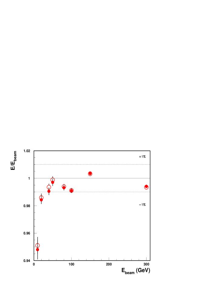
Figure 2: Energy linearity as a function of the beam energy for the $e/h$ method obtained using the iteration procedure with $\epsilon=0.1\%$ (black circles) and the first approximation (open circles).

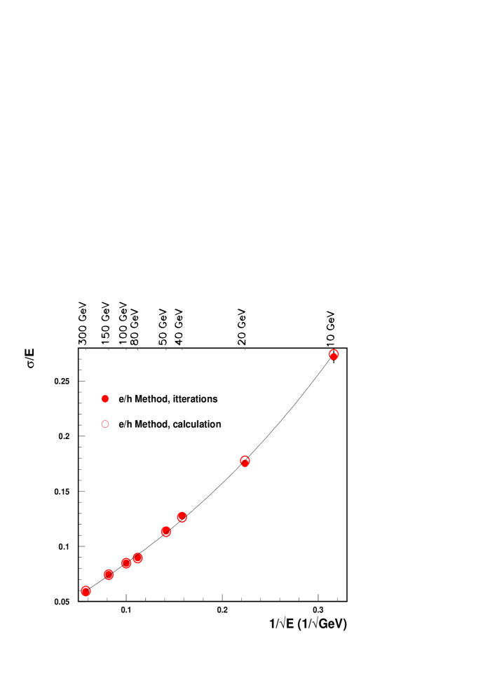
Figure 3: The fractional energy resolutions obtained with the $e/h$ method (black circles), and the first approximation (open circles).

We specially investigated the accuracy of the first approximation of energy, $E_{0}$. Fig. 2 shows the comparison between the energy linearities, the mean values of $E/E_{beam}$, obtained using the iteration procedure with $\epsilon=0.1\%$ (black circles) and the first approximation of energy (open circles). Fig. 3 shows the comparison between the energy resolutions obtained using these two approaches. As can be seen, the compared values are consistent within errors.

The suggested algorithm of the energy reconstruction can be used for the fast energy reconstruction in the first level trigger.

Table 2: Mean reconstructed energy, energy resolution and fractional energy resolution for the various beam energies obtained using the iteration procedure with $\epsilon=0.1\%$

$E_{beam}$	$E$ (GeV)	$\sigma$ (GeV)	$\sigma/E\ (\%)$
$10^{\ast}$ GeV	$9.30\pm 0.07$	$2.53\pm 0.05$	$27.20\pm 0.58$
$20^{\star}$ GeV	$19.44\pm 0.06$	$3.41\pm 0.06$	$17.54\pm 0.31$
40 GeV	$39.62\pm 0.11$	$5.06\pm 0.08$	$12.77\pm 0.21$
50 GeV	$49.85\pm 0.13$	$5.69\pm 0.13$	$11.41\pm 0.26$
80 GeV	$79.45\pm 0.16$	$7.14\pm 0.14$	$8.99\pm 0.18$
100 GeV	$99.10\pm 0.17$	$8.40\pm 0.16$	$8.48\pm 0.16$
150 GeV	$150.52\pm 0.19$	$11.20\pm 0.18$	$7.44\pm 0.12$
300 GeV	$298.23\pm 0.37$	$17.59\pm 0.33$	$5.90\pm 0.11$
∗The measured value of the beam energy is 9.81 $GeV$.
⋆The measured value of the beam energy is 19.8 $GeV$.

4.3 Energy Spectra

Fig. 4 and Fig. 5 show the pion energy spectra reconstructed with the $e/h$ method ($\epsilon=0.1\%$). The mean and $\sigma$ values of these distributions are extracted with Gaussian fits over $\pm 2\sigma$ range. The obtained mean values $E$, the energy resolutions $\sigma$, and the fractional energy resolutions $\sigma/E$ are listed in Table 2 for the various beam energies.

4.4 Energy Linearity

Fig. 6 demonstrates the correctness of the mean energy reconstruction. The mean value of $E/E_{beam}$ equals to $(99.5\pm 0.3)\%$ and the spread is $\pm 1\%$ except for the point at 10 $GeV$. But, as noted in [9], at this point the result is strongly dependent on the effective capability to remove events with interactions in the dead material upstream and to deconvolve the real pion contribution from the muon contamination. Fig. 6 and Fig. 7 compare the linearity, $E/E_{beam}$, as a function of the beam energy for the $e/h$ method, for the cells weighting method and for the benchmark method. For the cells weighting method the linearity is good to about $\pm 1\%$. The benchmark method (without rescaling) [10] badly reconstructs the beam energy: the reconstructed energy is systematically underestimated of about $30\%$, the linearity depends from the beam energy and the ratio $E/E_{beam}$ increases by $15\%$ from 20 to 300 $GeV$.

4.5 Energy Resolutions

Fig. 8 shows the fractional energy resolutions ($\sigma/E$) as a function of $1/\sqrt{E_{beam}}$ obtained by these three methods. As can be seen, the energy resolutions for the $e/h$ method (black circles) are comparable with the benchmark method (crosses) and only of $30\%$ worse than for the cells weighting method (open circles). A fit to the data points gives the fractional energy resolution for the $e/h$ method obtained using the iteration procedure with $\epsilon=0.1\%$

$$\frac{\sigma}{E}=\left[\frac{(58\pm 3)\%}{\sqrt{E}}+(2.5\pm 0.3)\%\right]\oplus\frac{(1.7\pm 0.2)\ GeV}{E}\ ,$$ (24)

for the $e/h$ method using the first approximation (22)

$$\frac{\sigma}{E}=\left[\frac{(56\pm 3)\%}{\sqrt{E}}+(2.7\pm 0.3)\%\right]\oplus\frac{(1.8\pm 0.2)\ GeV}{E}\ ,$$ (25)

for the benchmark method of

$$\frac{\sigma}{E}=\left[\frac{(60\pm 3)\%}{\sqrt{E}}+(1.8\pm 0.2)\%\right]\oplus\frac{(2.0\pm 0.1)\ GeV}{E}\ ,$$ (26)

and for the cells weighting method of

$$\frac{\sigma}{E}=\left[\frac{(42\pm 2)\%}{\sqrt{E}}+(1.8\pm 0.1)\%\right]\oplus\frac{(1.8\pm 0.1)\ GeV}{E}\ ,$$ (27)

where the symbol $\oplus$ indicates a sum in quadrature. As can be seen, the sampling term is consistent within errors for the $e/h$ method and the benchmark method and is smaller by 1.5 times for the cells weighting method. The constant term is the same for the benchmark method and the cells weighting method and is larger by $(0.7\pm 0.3)\%$ for the $e/h$ method. The noise term of about $1.8\ GeV$ is the same for these three methods that reflects its origin as the electronic noise. As to the two approaches for the $e/h$ method the fitted parameters coincides within errors.

5 Conclusions

The new simple method of the energy reconstruction for a combined calorimeter, the $e/h$ method, is suggested. It uses only the known $e/h$ ratios and the electron calibration constants and does not require the previous determination of any parameters by a minimization technique. The method has been tested on the basis of the 1996 test beam data of the ATLAS combined prototype calorimeter and demonstrated the correctness of the reconstruction of the mean values of energies. The obtained fractional energy resolution is $[(58\pm 3)\%/\sqrt{E}+(2.5\pm 0.3)]\oplus(1.7\pm 0.2)/E$. This algorithm can be used for the fast energy reconstruction in the trigger of the first level.

6 Acknowledgments

This work is the result of the efforts of many people from the ATLAS Collaboration. The authors are greatly indebted to all Collaboration for their test beam setup and data taking. Authors are grateful Peter Jenni and Marzio Nessi for fruitful discussion and support of this work. We are thankful Julian Budagov and Jemal Khubua for attention and support of this work.

Figure 4: The energy distributions for $E_{beam}$ = 10, 40 GeV (left column, up to down) and $E_{beam}$ = 20, 50 GeV (right column, up to down).

Figure 5: The energy distributions for $E_{beam}$ = 80, 150 GeV (left column, up to down) and $E_{beam}$ = 100, 300 GeV (right column, up to down).

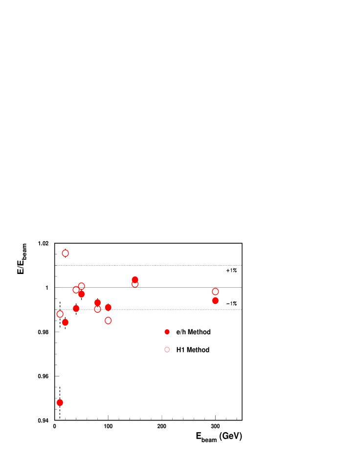
Figure 6: Energy linearity as a function of the beam energy for the $e/h$ method (black circles) and the cells weighting method (open circles).

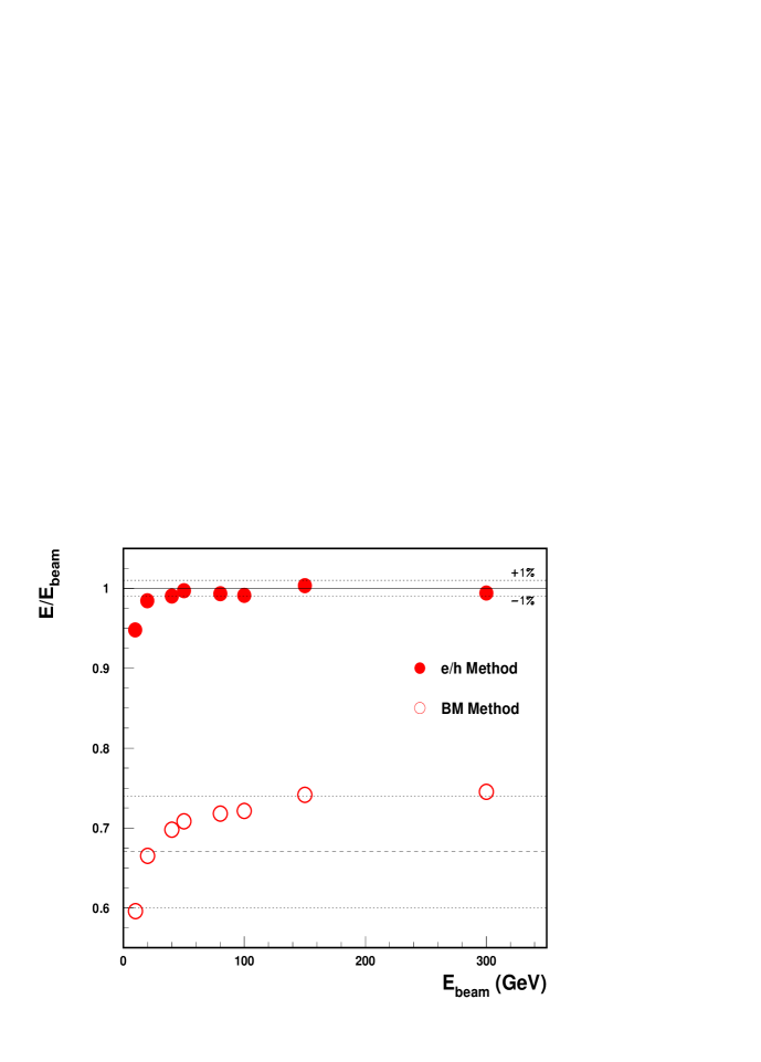
Figure 7: Energy linearity as a function of the beam energy for the $e/h$ method (black circles) and the benchmark method (open circles).

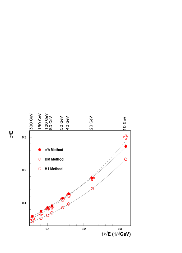
Figure 8: The energy resolutions obtained with the $e/h$ method (black circles), the benchmark method (crosses) and the cells weighting method (open circles).

References

- [1] ATLAS Collaboration, ATLAS Technical Proposal for a General Purpose pp Experiment at the Large Hadron Collider, CERN/LHCC/94-93, CERN, Geneva, Switzerland.
- [2] D.M. Gingrich , (RD3 Collaboration), NIM A364 (1995) 290;
- [3] ATLAS Collaboration, ATLAS TILE Calorimeter Technical Design Report, CERN/LHCC/96-42, ATLAS TDR 3, 1996, CERN, Geneva, Switzerland.
- [4] O. Gildemeister, F. Nessi-Tedaldi and M. Nessi, Proc. 2nd Int. Conf. on Calorimetry in High Energy Physics, Capri, 1991.
-
[5]
F. Ariztizabal , (RD34 Collaboration), NIM (1994) 384;
E.Berger, , (RD34 Collaboration), LRDB Status Report, CERN/ LHCC 95-44. -
[6]
M. Bosman , (RD34 Collaboration), CERN/DRDC/93-3 (1993);
F. Ariztizabal , (RD34 Collaboration), CERN/DRDC/94-66 (1994). - [7] S. Agnvall , Hadronic Shower Development in Iron-Scintillator Tile Calorimetry, NIMA (in press); LANL e-print Archive hep-ex/9904032.
- [8] J.A. Budagov, Y.A. Kulchitsky, V.B. Vinogradov , JINR-E1-97-318, 1997, JINR, Dubna, Russia; ATLAS Internal note, TILECAL-No-127, 1997, CERN, Geneva, Switzerland.
- [9] M. Cobal , ATL-TILECAL-98-168, 1998, CERN, Geneva, Switzerland.
- [10] ATLAS Collaboration (Calorimetry and Data Acqusition), S. Akhmadaliev , Results from an Expanded Combined Test of the Electromagnetic Liquid Argon Calorimeter with a Hadronic Scintillating-Tile Calorimeter, NIMA (in press).
- [11] Z. Ajaltouni , NIM A387 (1997) 333.
- [12] M.P. Casado and M. Cavalli-Sforza, ATLAS Note, TILECAL-NO-75 (1996) CERN, Geneva, Switzerland.
- [13] T.A. Gabriel , NIM A295 (1994) 336.
- [14] R. Wigmans, NIM A265 (1988) 273.
- [15] D. Groom, Proceedings of the Workshop on Calorimetry for the Supercollides, Tuscaloosa, Alabama, USA, 1989.
- [16] Y.A. Kulchitsky, M.V. Kuzmin, V.B. Vinogradov, JINR-E1-99-303, 1999, JINR, Dubna, Russia; ATL-TILECAL-99-026, 1999, CERN, Geneva, Switzerland.