Atmospheric Neutrinos and the Oscillations Bonanza

W. Anthony Mann
Department of Physics, Tufts University
Medford, MA 02155, USA

New observations with atmospheric neutrinos from the underground experiments SuperKamiokande,  Soudan 2,  and MACRO,  together with earlier results from Kamiokande and IMB, are reviewed. The most recent observations reconfirm aspects of atmospheric flavor content and of zenith angle distributions which appear anomalous in the context of null oscillations. The anomalous trends, exhibited with high statistics in both sub-GeV and multi-GeV data of the SuperKamiokande water Cherenkov experiment, occur also in event samples recorded by the tracking calorimeters. The data are well-described by disappearance of $\nu_{\mu}$ flavor neutrinos arising in oscillations with dominant two-state mixing, for which there exists a region in ($\sin^{2}2\theta$, $\Delta m^{2}$) allowed by all experiments. In a new analysis by SuperKamiokande, $\nu_{\mu}\rightarrow\nu_{\tau}$ is favored over $\nu_{\mu}\rightarrow\nu_{sterile}$ as the dominant oscillation based upon absence of oscillation suppression from matter effects at high energies. The possibility for sub-dominant $\nu_{\mu}\rightarrow\nu_{e}$ oscillations in atmospheric neutrinos which arises with three-flavor mixing, is reviewed, and intriguing possibilities for amplification of this oscillation by terrestrial matter-induced resonances are discussed. Developments and future measurements which will enhance our knowledge of the atmospheric neutrino fluxes are briefly noted.

1 Atmospheric Neutrino Beamline

We are lucky, you and I, to be born here on planet Earth and to have as our birthright the unrestricted use of a splendid neutrino beamline. Truly remarkable is that the originating hadronic primary beam, namely the cosmic ray flux of protons and assorted stable nuclei, is isotropic to high degree. Moreover the beamline target region, which is the terrestrial atmosphere, is very nearly spherically symmetric. Together these two attributes ensure that neutrino fluxes of this beamline, in the absence of neutrino oscillations, must be up/down symmetric with respect to the horizon [2, 3]. Consequently, observation of a sizable neutrino flux up/down asymmetry by the user community is clear evidence that new physics is happening with neutrinos. The null oscillation up/down symmetry for neutrino fluxes is however not complete. There are geomagnetic effects which produce mild distortions in the fluxes of low energy neutrinos and of horizontal neutrinos. These distortions, which are latitude-dependent, provide useful tests for data verity. The beamline delivers neutrino fluxes which are wide-band in $E_{\nu}$ and which contain the flavors $(\nu_{\mu}+\overline{\nu}_{\mu})$ and $(\nu_{e}+\overline{\nu}_{e})$. In the absence of oscillations these flavors must occur in the ratio 2:1 for sub-GeV neutrinos; for multi-GeV neutrinos the ratio should increase gradually with $E_{\nu}$. At or below the Earth’s surface the atmospheric flux is about $10^{3}$ $\nu$’s incident per human body per second [3], an amount which is adequate for experimentation but does not pose a radiation safety hazard. The neutrino path lengths $L$ which are possible in this beamline range from 20 km for $\nu$’s incident from the local zenith, to 13,000 km for $\nu$’s arriving from the opposite side of the globe. Within the beamline there are regions of different, roughly uniform, matter densities. These include the Earth’s mantle (density $\simeq$ 4.5 $g/cm^{3}$) and the Earth’s core (density $\simeq$ 11.5 $g/cm^{3}$). This arrangement may eventually permit experimental strategies to be tried which are akin to utilization of regeneration plates in $K^{0}$ beams. The neutrinos from this ever-running beamline give rise to useful reaction final states both in and below any detector deployed underground. By investigating the full panoply of event types possible with charged current (CC) or neutral current (NC) interactions, experimentalists can explore the physics of atmospheric neutrinos for incident $E_{\nu}$ ranging from 100-200 MeV up to and exceeding 1000 GeV.

2 Oscillation Phenomenology

We believe there to be three active neutrinos; there may be sterile ones $\nu_{s}$ as well. For the active neutrinos, the weak flavor eigenstates $\nu_{e}$, $\nu_{\mu}$, and $\nu_{\tau}$ are related to the mass eigenstates according to a product involving the unitary mixing matrix $U$:

$$\left[\begin{array}[]{c}\nu_{e}\\ \nu_{\mu}\\ \nu_{\tau}\end{array}\right]=\left[\begin{array}[]{ccc}U_{e1}&U_{e2}&U_{e3}\\ U_{\mu 1}&U_{\mu 2}&U_{\mu 3}\\ U_{\tau 1}&U_{\tau 2}&U_{\tau 3}\\ \end{array}\right]\left[\begin{array}[]{c}\nu_{1}\\ \nu_{2}\\ \nu_{3}\end{array}\right].$$ (1)

The oscillation probabilities which follow from this can, in principle, involve numerous competing processes:

$$P(\nu_{\alpha}\rightarrow\nu_{\beta})=\delta_{\alpha\beta}-4\sum_{i=1}^{3}\sum_{j=i+1}^{3}U_{\alpha i}\cdot U_{\beta i}\cdot U^{*}_{\alpha j}\cdot U^{*}_{\beta j}\cdot\sin^{2}\left[\frac{1.27\mbox{ }\Delta m^{2}_{ij}\cdot L}{E_{\nu}}\right].$$ (2)

Fortunately there are cases wherein oscillations decouple so that the situation is well-described by two-neutrino oscillations, for which the mixing matrix is much simpler:

$$\left[\begin{array}[]{c}\nu_{\alpha}\\ \nu_{\beta}\end{array}\right]=\left[\begin{array}[]{cc}\cos\theta&\sin\theta\\ -\sin\theta&\cos\theta\end{array}\right]\left[\begin{array}[]{c}\nu_{1}\\ \nu_{2}\end{array}\right].$$ (3)

The probability for oscillation between the two participating flavors can then be written using the well-known expression

$$P(\nu_{\alpha}\rightarrow\nu_{\beta})=\sin^{2}(2\theta)\cdot\sin^{2}\left[\frac{1.27\mbox{ }\Delta m^{2}[\mbox{eV}^{2}]\cdot L\mbox{[km] }}{E_{\nu}\mbox{[GeV] }}\right].$$ (4)

It is convenient to define the vacuum oscillation length $L_{0}$:

$$L_{0}\mbox{[km] }=\pi\left[\frac{1.27\mbox{ }\Delta m^{2}}{E_{\nu}}\right]^{-1}=2.47\frac{E_{\nu}\mbox{[GeV] }}{\Delta m^{2}[\mbox{eV}^{2}]}.$$ (5)

The oscillation phase can then be expressed as ($\pi L/L_{0}$).

3 The Underground Detectors

Currently there are three underground experiments which are accumulating atmospheric neutrino data. The premier detector in this field is SuperKamiokande (Super-K). It is a 50 kiloton water Cherenkov detector deployed in a configuration of two concentric cylindrical volumes. The inner volume is the 22.5 kiloton fiducial region, while the surrounding outer volume is used to veto entering tracks and to tag exiting tracks. Flavor tagging of events is based upon the relative sharpness or diffuseness of Cherenkov rings, with muon tracks yielding sharp rings, and electrons yielding diffuse ones [4]. The analyzed exposure for Super-K in-detector neutrino reactions reported here is from 848 livedays; this corresponds to a whopping 52 fiducial kiloton years!

MACRO and Soudan 2 are tracking calorimeter detectors. MACRO is a large-area, planar tracker. It is optimized for tracking in vertical directions and is sufficiently massive (about 5.3 kilotons) to be effective as a neutrino detector. Charged particle tracking is carried out using horizontal layers of streamer tubes with wire and stereo strip readout. Three horizontal planes and also vertical walls of liquid scintillator counters provide timing information with resolution of about 0.5 nsec [5]. MACRO has the largest rock overburden of the three underground experiments, consequently the flux of downgoing muons which can give rise to backgrounds is lowest at its site [6].

Soudan 2 is a fine-grained iron tracking calorimeter of total mass 963 tons which images non-relativistic as well as relativistic charged particles produced in neutrino reactions. The detector operates as a slow-drift time projection chamber. Its tracking elements are meter-long plastic drift tubes which are placed into the corrugations of steel sheets. The sheets are stacked to form a tracking lattice of honeycomb geometry. A stack is packaged as a calorimeter module and the detector is assembled building-block fashion using these modules. The calorimeter is surrounded on all sides by a cavern-liner active shield array of two or three layers of proportional tubes [7]. The contained event sample reported here is obtained from a 4.6 fiducial kton-year exposure.

4 Atmospheric Neutrino Flavor Ratio

A hypothesis test of long-standing for the existence of anomalous behavior of atmospheric neutrinos is “the flavor ratio” for which updated measurements have become available this summer. Atmospheric neutrinos are produced almost entirely in pion - muon decay chains initiated by cosmic ray interactions in the upper atmosphere. As a consequence, $(\nu_{\mu}+\overline{\nu}_{\mu})$ versus $(\nu_{e}+\overline{\nu}_{e})$ neutrino flavor rates occur in a ratio 2:1. The underground experiments examine the ratio-of-ratios $R$, which is $(\nu_{\mu}+\overline{\nu}_{\mu})/(\nu_{e}+\overline{\nu}_{e})$ from the data, divided by the same ratio from a Monte Carlo. In the absence of new physics the ratio-of-ratios should be unity; and so the degree to which deviation from unity is observed is a measure of anomalous behavior of the fluxes. In actual practice, the experiments measure a related quantity, $R^{\prime}$, the ratio of observed event counts. For the Super-K water Cherenkov experiment, $R^{\prime}$ is the ratio of single-ring $\mu$-like to $e$-like events in the data divided by $\mu$-like to $e$-like from the Monte Carlo [8]. For Soudan 2, $R^{\prime}$ is the ratio of single-track to single-shower events for the data, divided by the same ratio from the Monte Carlo [9].

Here, then, are the latest results from Super-K, updated to include the 848 day exposure: For the “sub-GeV” sample (with event visible energy $E_{vis}$ $<$ 1.33 GeV),

$$R^{\prime}(\mu\mbox{-ring}/e\mbox{-ring})=0.68\pm 0.02\mbox{ (stat.) }\pm 0.05\mbox{ (syst.) }.$$

For the “multi-GeV” sample ($E_{vis}>$ 1.33 GeV),

$$R^{\prime}(\mu\mbox{-ring}/e\mbox{-ring})=0.68\pm 0.04\pm 0.08.$$

From the Soudan 2 iron calorimeter there is an updated measurement based upon contained track and shower events of a 4.6 fiducial kiloton year exposure. The events occur mostly within the sub-GeV regime as defined by Super-K:

$$R^{\prime}(trk/shwr)=0.68\pm 0.11\pm 0.06.$$

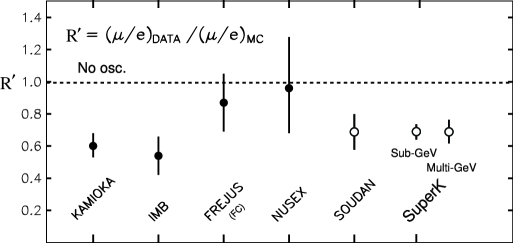
Figure 1: Measurements of the atmospheric neutrino flavor ratio of ratios [14].

Measurements of the atmospheric flavor ratio have been accumulating from the underground experiments for more than a decade [10, 11, 12, 13]. These most recent results reconfirm the atmospheric anomaly as first reported years ago by the water Cherenkov experiments Kamiokande and IMB. Fig. 1 shows that the various $R^{\prime}$ measurements, by different experiments with different techniques and systematics, give a consistent picture. The flavor content of the atmospheric neutrino flux is anomalous but in a way that is readily understandable, if indeed muon neutrinos are being depleted by $\nu_{\mu}\rightarrow\nu_{x}$ oscillations over pathlengths which occur in the terrestrial beamline.

5 Zenith Angle Distortions and Super-K Data

To elicit the pathlength $L$ dependence which, in an oscillation scenario, will correlate with ($\nu_{\mu}+\overline{\nu}_{\mu}$) disappearance, we consider the distributions of neutrino zenith angle which have been obtained for fully contained (FC) and for partially contained (PC) events in the SuperKamiokande experiment. In evaluating zenith angle distributions and also flavor ratios, it is useful to keep in mind trends which are shown by the survival probability curves in Fig. 2a for $\nu_{\mu}$ neutrinos [15]. The curves depict the probability for $\nu_{\mu}\rightarrow\nu_{\mu}$ from an atmospheric flux for which $\cos\theta_{z}$ at 1.0 is vertically downgoing and $\cos\theta_{z}$ at -1.0 is vertically upgoing. The curves are drawn for “representative” $\nu_{\mu}\rightarrow\nu_{x}$ parameter settings which we use again in paragraphs below, namely $\sin^{2}2\theta=1.0$ and $\Delta m^{2}=5\times 10^{-3}$ eV². The oscillation pattern in Fig. 2a evolves in a regular way with increasing energy of the neutrino. For $E_{\nu}$ of 250 MeV, the first oscillation swing severely depletes the downward-going flux, and rapid oscillations deplete the flux incident from below-horizon; the net result is a substantial average depletion at all incident angles. At energies above 1 GeV however the depletion moves almost entirely to the $\nu_{\mu}$ flux incident from below-horizon, and this situation remains for $E_{\nu}$ increasing to 30 GeV. At higher $E_{\nu}$ the pattern shifts to beyond range, and $\nu_{\mu}$ depletion ceases because our planet is not big enough to accomodate the first oscillation swing.

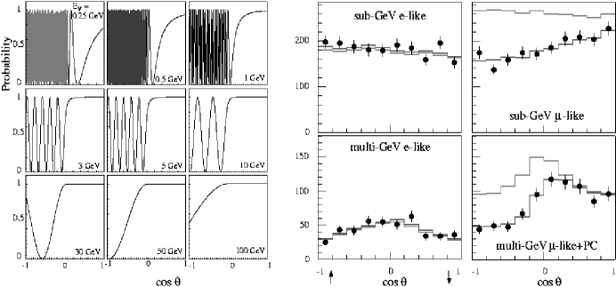
Figure 2: a (left): Survival probability curves for mono-energetic, isotropic fluxes of muon neutrinos with $\nu_{\mu}\rightarrow\nu_{\tau}$ and $\sin^{2}2\theta=1.0$, $\Delta m^{2}=5\times 10^{-3}$ eV² for nine values of $E_{\nu}$. b (right): Super-K distributions for $\cos\theta_{z}$ single ring $e$-like and $\mu$-like events. Expectations for null oscillation and for $\nu_{\mu}\rightarrow\nu_{\tau}$ are shown by gray-line and solid-line histograms respectively.

Distributions showing ten bins in $\cos\theta_{z}$ for events of the 848-day Super-K exposure are given in Fig. 2b. The $\nu_{e}$ and $\nu_{\mu}$ flavor samples are shown separately and are subdivided according to $E_{vis}$. The $\nu_{e}$ events show no angular distortion in either the sub-GeV or multi-GeV regimes. In striking contrast the $\nu_{\mu}$ samples show large regions of disappearance, the samples being depleted relative to expectations of the null oscillation Monte Carlo (gray-line histograms). The depletions exhibit dependence on zenith angle and therefore on path length $L$. Additionally, the depleted regions are of different character in the sub-GeV and multi-GeV sets. At sub-GeV energies the $\mu$-like events appear depleted at all angles including those with incidence from above horizon. At multi-GeV energies however, the depletion is mostly restricted to incidence from below-horizon. Although the correlation between the final state lepton and the initial neutrino direction is relatively poor for sub-GeV compared to multi-GeV data, nevertheless the trend is suggestive of a dependence on $E_{\nu}$ for $\nu_{\mu}$ flavor disappearance. As shown by the solid-line histograms superposed in Fig. 2b, the zenith angle distortions of the $\nu_{\mu}$ flavor samples are well-described by a fit of two-state $\nu_{\mu}\rightarrow\nu_{\tau}$ neutrino oscillations (discussed below). Contrastingly, the $\nu_{e}$ samples are in agreement with the null oscillation Monte Carlo (MC) to a degree which is perhaps disappointing. With multi-GeV $\nu_{e}$’s which presumably traversed the Earth’s core, for example, no irregularity is apparent; there are no hints anywhere to suggest $\nu_{\mu}\rightarrow\nu_{e}$ oscillations.

The depletion of $\nu_{\mu}$ neutrinos can be shown in an informative way by plotting the asymmetry in zenith angle as a function of event momentum as in Fig. 3a. The asymmetry $A$ is defined $A=(U-D)/(U+D)$, where $U$ is the number of events with upward incidence at angles $\cos\theta>0.2$ and $D$ equals events with downward incidence at angles $\cos\theta<-0.2$. For the single-ring $e$-like events, $A$ $\simeq$ 0 at all momenta. For the $\mu$-like events however, $A$ becomes increasingly negative, there being a dearth of upward-going versus downward-going neutrinos which becomes more pronounced with increasing momentum. For the multi-GeV sample the value of $A$ is $-0.32\pm 0.04\pm 0.01$, which is nearly eight standard deviations from zero asymmetry.

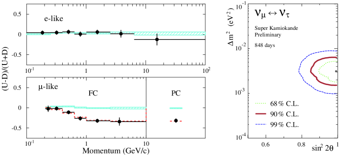
Figure 3: a (left): Zenith angle asymmetry versus event momentum for single ring $e$-like and $\mu$-like events of Super-K. b (right): Super-K allowed region in the neutrino oscillation parameter space for $\nu_{\mu}\rightarrow\nu_{\tau}$ mixing, based upon the $\chi^{2}$ fit to FC and PC single ring event distributions.

For the fully-contained and partially contained single-ring data just shown, the Super-K collaboration uses a $\chi^{2}$ function to determine the oscillation parameters of two-state mixing:

$$\chi^{2}(\sin^{2}2\theta,\Delta m^{2},\vec{\varepsilon})=\sum_{i=1,70}\frac{(N^{i}_{data}-N^{i}_{MC})^{2}}{\sigma^{2}_{i}}+\sum_{j}\frac{\varepsilon^{2}_{j}}{\sigma^{2}_{j}}.$$ (6)

For this purpose the $\mu$-like and the $e$-like samples are sub-divided using five bins in $\cos\theta_{z}$ and seven bins in momentum. The $\chi^{2}$ is the sum of data minus MC expectation squared over the 70 bins, where the MC is a function of the oscillation parameters $\sin^{2}2\theta$, $\Delta m^{2}$, and parameters $\varepsilon_{j}$ which allow for systematic effects. The $\varepsilon_{j}$ include the parameter $\alpha$ which appears in the flux normalization factor (1 + $\alpha$). At each point in the plane of $\sin^{2}2\theta$ and $\Delta m^{2}$, the $\chi^{2}$ is minimized with respect to the $\varepsilon_{j}$ parameters; the minimum $\chi^{2}$ point (best fit) is then obtained. Contours for allowed regions at 68%, 90%, and 99% CL are obtained on the basis of $\chi^{2}-\chi^{2}_{minimum}$ as shown in Fig. 3b. The $\nu_{\mu}\rightarrow\nu_{\tau}$ oscillation best fit yields $\chi^{2}$ = 55/67 d.o.f. and fares much better than the null oscillation fit having 177/69 d.o.f. At the best fit point the oscillation parameter values are $\sin^{2}2\theta=0.99$ and $\Delta m^{2}=3.1\times 10^{-3}$ [eV²]; the MC flux normalization is shifted upwards ($\alpha$ = +0.05) relative to the absolute rate based upon the Honda et al. fluxes for the Super-K site [16]. It is comforting to see that $\sin^{2}2\theta$ from the best fit with Super-K FC and PC events now occurs in the physical region, for this has not always been the case in the past.

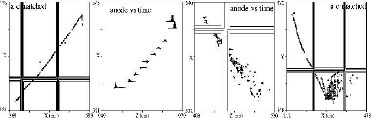
Figure 4: Two track-plus-recoil events, a single shower event, and a $\overline{\nu}_{\mu}$ flavor multiprong event, recorded in Soudan 2.

6 Contained Events in Soudan 2

Concerning evidence for neutrino oscillations carried by in-detector neutrino interactions, a “second look” is afforded by the fully contained track, shower, and multiprong events recorded by Soudan 2. Projected images of “typical” data events are shown in Fig. 4; these include two examples of muon tracks with companion recoil protons ($\nu_{\mu}$ quasi-elastics), a shower event ($\nu_{e}$ quasi-elastic), and a $\overline{\nu}_{\mu}$-flavor multiprong.

The approach taken by Soudan 2 is to isolate a sub-sample of events for which $L/E_{\nu}$ can be measured with good resolution on an event-by-event basis, thereby allowing the oscillation analysis to be carried out directly using $L/E_{\nu}$ distributions. In a fine-grain tracking calorimeter, $E_{\nu}$ can be reliably estimated based upon $E_{vis}$. To ensure good resolution for ascertaining the incident neutrino direction, quasi-elastic single track and shower events are selected which have measurable recoil protons. Otherwise, in the absence of a visible recoil, the lepton energy is required to exceed 600 MeV. Multiprong events are also selected, provided that $E_{vis}>$ 700 MeV and $|\Sigma\vec{p}_{vis}|>$ 450 MeV/$c$ and $P_{lept}>$ 250 MeV/$c$. The momentum requirements improve the resolution of neutrino direction and ensure reliable flavor-tagging for charged current events (success probability $>$ 0.92). For the $\nu_{\mu}$ ($\nu_{e}$) sample, $\Delta E/E$ is 20% (23%). For pointing of the event along the original neutrino direction, the resolutions are of order 20-30 degrees which is quite respectable for a sub-GeV data set [17].

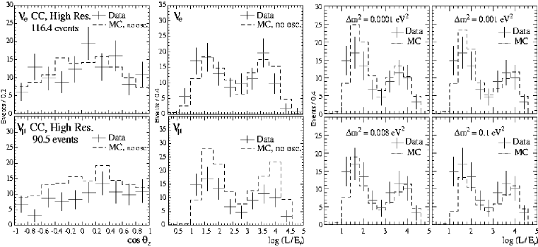
Figure 5: a (left): Distributions in $\cos\theta_{z}$ for $\nu_{e}$ and $\nu_{\mu}$ flavor event samples. Data (crosses) are compared to the null oscillation MC (dashed histogram) where the MC has been rate normalized to $\nu_{e}$ data. b (middle): Distributions of $\log(L/E_{\nu})$ for $\nu_{e}$ and $\nu_{\mu}$ charged current events compared to the neutrino MC with no oscillations; the MC has been rate-normalized to the $\nu_{e}$ data. c (right): Comparison of $L/E_{\nu}$ distribution for $\nu_{\mu}$ data (crosses) and expectations from neutrino oscillations for four $\Delta m^{2}$ values, with $\sin^{2}2\theta=1.0$.

Zenith angle distributions for the resolution-enhanced (HiRes) $\nu_{e}$ and $\nu_{\mu}$ samples are shown in Fig. 5a, where the MC rates have been normalized to the observed number of $\nu_{e}$ events. For the $\nu_{e}$ sample, the zenith angle distribution follows the shape predicted by the MC without oscillations. The corresponding $\nu_{\mu}$ data distribution however consistently falls below the MC expectation. The dearth is mild but discernible for $\nu$ incidence above the horizon and becomes more pronounced with below-horizon incidence. These features are in agreement with those exhibited with much higher statistical weight by the sub-GeV FC single-ring events of Super-K.

Distributions in $\log L/E_{\nu}$ for the HiRes $\nu_{e}$ and $\nu_{\mu}$ samples are shown in Fig. 5b wherein the data (crosses) are compared to the null oscillation MC. The peaks at low $\log L/E_{\nu}$ are populated by down-going neutrinos incident from above-horizon; the lower flux central regions are populated by horizontal neutrinos, while the peaks at higher $\log L/E_{\nu}$ contain neutrinos traveling upward through the Earth. To within statistical fluctuations, the $\nu_{e}$ sample follows the null oscillation MC expectation. For the $\nu_{\mu}$ sample, there is a depletion which pervades the entire up-going region and extends into the down-going flux, subsiding only in the lowest $L/E_{\nu}$ bins which contain the most vertically down-going events.

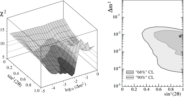
Figure 6: a (left): $\chi^{2}$ “map” over the $\Delta m^{2}$, $\sin^{2}2\theta$ plane; the MC normalization is also allowed to adjust. Contour boundaries are approximately 68% CL, 90% CL, and 95% CL based upon $\chi^{2}_{min}$ plus 2.30, 4.61, and 5.99 respectively. b (right): Soudan 2 allowed regions for $\nu_{\mu}\rightarrow\nu_{x}$ oscillations at approximately 68% and 90% CL.

The $\log L/E_{\nu}$ distributions from data can be fitted to oscillation-weighted MC events using a $\chi^{2}$ constructed similarly to the function utilized by Super-K. An exploratory matchup is shown in Fig. 5c, for which $\sin^{2}2\theta$ is set to 1.0 and the $\nu_{\mu}$ data is displayed together with weighted MC distributions for $\nu_{\mu}\rightarrow\nu_{x}$ oscillations at four different $\Delta m^{2}$ values. At $\Delta m^{2}=10^{-4}$ eV² the oscillation solution exceeds the data in the down-going hemisphere. At $\Delta m^{2}=10^{-3}$ eV² the matchup improves, and at $\Delta m^{2}=8\times 10^{-3}$ eV² the oscillation solution follows the data rather well. However $\Delta m^{2}=10^{-1}$ eV², is “too far” - the oscillation solution falls below the data in the down-going hemisphere and in the up-going hemisphere as well. This sequence illustrates key features of the $\chi^{2}$ mapping of the ($\Delta m^{2}$, $\sin^{2}2\theta$) plane shown in Fig. 6a. The best fit lies in the darkened basin region of the contour. The boundaries of the different shaded areas correspond to regions allowed at approximately 68%, 90%, and 95% CL.

In the contour map there appears a ‘ridge of improbability’ at $\Delta m^{2}$ lying just above the best fit ‘basin’. This region corresponds to oscillation solutions for which the first oscillation swing should create a depletion in the downward-going $\nu_{\mu}$ flux. No such depletion occurs in the data and since the events have sufficient directional resolution to show it if it occurred, the $\chi^{2}$ becomes large there. The projection of the $\chi^{2}$ contours onto the ($\Delta m^{2}$, $\sin^{2}2\theta$) plane is shown in Fig. 6b. The minimum $\chi^{2}$ point is at $\sin^{2}2\theta=0.95$ and $\Delta m^{2}=0.8\times 10^{-2}$ eV². The flux normalization, which is allowed to vary in the fitting, is reset at the minimum $\chi^{2}$ point to 0.82 times the absolute event rate based upon the Monte Carlo. The Monte Carlo utilizes the 1989 Bartol flux calculation for the Soudan site [18].

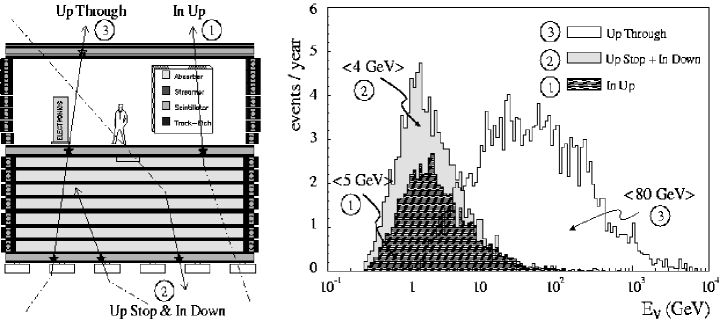
Figure 7: a (left): Cross section sketch of the MACRO detector, illustrating the event topologies of partially contained and through-going $\nu_{\mu}$ samples. b (right): Distributions of parent neutrino energies for the three neutrino samples of MACRO.

7 Partially Contained Events in MACRO

Although the Soudan results are in general agreement with the neutrino oscillation effects reported by Super-K, they do not at present confirm the striking depletion in upgoing muon neutrinos shown by Super-K’s multi-GeV events. Fortunately, event samples which provide another, independent viewing of the multi-GeV $E_{\nu}$ regime are being accumulated in the MACRO experiment [19].

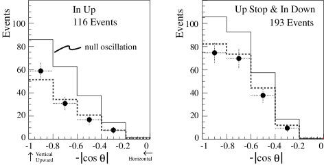
Figure 8: Distributions in $\cos\theta_{z}$ for MACRO partially contained events. The data (solid circles) are seen to fall below the null oscillation expection in every bin of both samples.

Fig. 7a shows the three $\nu_{\mu}$ CC event categories studied by MACRO. These include: i) “In-Up” events, which are $(\nu_{\mu}+\overline{\nu}_{\mu})$ reactions occurring inside the detector creating muons which exit through the top; ii) “Up-Stop” and “In-Down” events which are classified on the basis of topology (timing information not available) and which are analyzed together; and iii) “Up-Through muons” which are initiated by high energy $(\nu_{\mu}+\overline{\nu}_{\mu})$ interactions below the detector creating muons which traverse the detector from bottom to top. Parent neutrino energy distributions for each of the three event categories are shown in Fig. 7b.

The In-Up events, and also the Up-Stop plus In-Down events, probe the multi-GeV $E_{\nu}$ regime; the mean $E_{\nu}$ values for these two MACRO samples are 5 GeV and 4 GeV respectively. Zenith angle distributions for these partially contained samples are shown in Fig. 8. The event populations are binned in $\cos\theta_{z}$ from the horizontal at $\cos\theta_{z}=0.0$, to vertically upward at zenith cosine -1.0. For the 116 events of the In-Up sample shown in Fig. 8a, the data fall below the null oscillation Monte Carlo in every bin. (Note that the acceptance for this planar calorimeter is relatively lower for horizontal directions.) The ratio of In-Up events observed to the MC prediction, is $0.57\pm 0.16$. Thus the In-Up sample exhibits the large-scale depletion for multi-GeV upward going events seen in the Super-K data. The data are seen to distribute in accord with the oscillation best fit based upon MACRO Up-Through muons which is described in the next Section. A similar trend is observed with the Up-Stop and In-Down sample shown in Fig. 8b. Since the latter sample contains roughly equal portions of Up-Stop events which are fully oscillating and of In-Down events from above horizon which are not oscillating, the amount of depletion relative to null oscillation is reduced compared to that of the In-Up sample.

8 Upgoing Muons in Super-K and MACRO

There are two event samples which are initiated by below-detector $(\nu_{\mu}+\overline{\nu}_{\mu})$ interactions, namely upward stopping muons and upward through-going muons, and they represent two different portions of the neutrino spectrum. This can be seen from comparison of $E_{\nu}$ distributions (2) and (3) of Fig. 7b, which roughly characterize the muon samples in Super-K as well as in MACRO. The $E_{\nu}$ spectrum (2) which produces upward stopping muons is distinctly lower, with the bulk of the spectrum lying below 40 GeV. The different $E_{\nu}$ regimes give rise to rather different oscillation behavior, as can be seen by evaluation of the phase angle in Eq. (4) at our nominal $\nu_{\mu}\rightarrow\nu_{\tau}$ parameter values $\sin^{2}2\theta=1.0$ and $\Delta m^{2}=5\times 10^{-3}$ eV². At $E_{\nu}$ = 40 GeV, the vacuum oscillation length $L_{0}$ equals 1.5 Earth diameters. Recall that $L_{0}$ is proportional to $E_{\nu}$ and that the oscillation phase is $\pi L/L_{0}$. Then for $E_{\nu}$ much larger than 40 GeV as in the case for many through-going muon events, $L_{0}$ exceeds the Earth’s diameter. The result is that $\nu$’s initiating through-going muons generally have small oscillation phase angles and hence give rise to low oscillation probabilities. On the other hand, for up-stopping muons, $E_{\nu}<$ 40 GeV and neutrino $L_{0}$ values are less than $L$ values so that sizable phases and large oscillation probabilities frequently occur.

The expectation that oscillation will occur in relatively different proportions in up-stopping versus upward through-going muon samples has been examined by Super-K. This is done by measuring the upward-stopping to up-through ratio of muon fluxes. In the presence of the two-state mixing inferred from the in-detector samples of Sect. 6, the muon stop/thru ratio should fall below the MC prediction for null oscillation. Fig. 9a shows the stop/thru ratio plotted versus $\cos\theta_{z}$ for muons incident from the horizontal ($\cos\theta_{z}=0.0$) to those most vertically upgoing ($\cos\theta_{z}=-1.0$). The observed stop/thru ratio is 0.24 $\pm$ 0.02 which is 2.8 standard deviations below the null oscillation expectation of 0.37 $\pm$ 0.05.

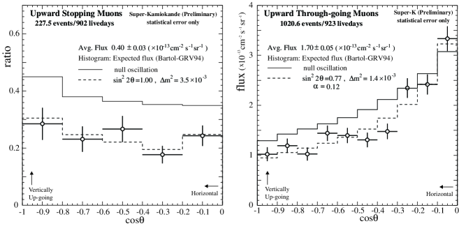
Figure 9: a (left): Ratio of upward-stopping to through-going muons versus $\cos\theta_{z}$ observed in Super-K. The data ratio falls below the null oscillation expectation for each of the five below-horizon bins. b (right): The upward through-going muon flux versus zenith angle observed in Super-K. The shape of the data distribution (open circles) differs from the null oscillation expectation (solid histogram) and is better described by two-state oscillations (dashed histogram).

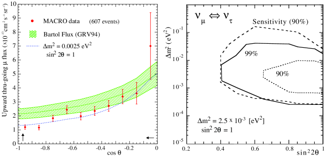
Figure 10: a (left): The angular distribution of upward through-going muons observed in MACRO. The data distribution (solid circles) differs from the null oscillation expectation (shaded band) in shape and in rate. b (right): The neutrino oscillation allowed regions obtained by MACRO from the upward through-going muons. Confidence level and experimental sensitivity boundaries are calculated using the Feldman-Cousins method.

Additional information can be gleaned from the upward through-going muons alone. These events arise from neutrino interactions which have the highest range for parent $E_{\nu}$. To see how oscillations affect this sample, consider $E_{\nu}$ at 100 GeV, which is the mean energy estimated for Super-K events. (However the distribution of parent energies is broad and extends above 1000 GeV.) At our representative parameter settings, the vacuum oscillation length is approximately $1.2\pi$ times the Earth diameter; consequently the phase angle of the flavor oscillation probability is $L/1.2$ in units of Earth diameter. For horizontal muons the flight paths of parent neutrinos are of order 500 km or 0.04 Earth diameters, and so the neutrino phase angles will be too small to induce significant oscillation probability. However for vertical muons the neutrino paths $L$ become comparable to the Earth’s diameter, and the phase angles become sufficiently large that rapid oscillation swings ensue. ( For $E_{\nu}<100$ GeV, oscillations will also occur for muons incident away from the vertical. )

Available for this conference is an updated through-going muon sample exceeding one thousand events from Super-K, the zenith angle distribution of which is shown in Fig. 9b. (This sample is noticeably larger than the one published this spring from a 537 day exposure [20].) Fig. 9b exhibits the trends implied by oscillations for this sample: For bins which are just below the horizon, the data agree with the Monte Carlo expectation for null oscillation. For the bins below $\cos\theta_{z}=-0.3\mbox{ }$ however, the data fall below the null oscillation prediction and this trend continues with muons of more vertical inclination. That is, the shape of the zenith angle distribution of these upward throughgoing muons, and their overall flux rate as well, deviate significantly from null oscillation and agree with expectations from $\nu_{\mu}\rightarrow\nu_{\tau}$ mixing as inferred from in-detector neutrino interactions.

The same features are seen in the angular distribution of upward through-going muons recorded by MACRO [21] as shown in Fig. 10a. The ratio of data to the MC prediction for MACRO is $0.74\pm 0.03\pm 0.04\pm 0.12$; the last term containing the largest uncertainty reflects limited knowledge of the absolute neutrino flux and of deep inelastic neutrino cross sections.

Fig. 10b shows the allowed region of the oscillation parameters obtained by MACRO based upon the upward through-going muon sample. The allowed region is calculated using the Feldman-Cousins method [22]. For the MACRO data, the minimum $\chi^{2}$ point ($\chi^{2}$ of 10.6) is in the unphysical region at $\sin^{2}2\theta=1.5$ . To clarify the situation, the experimental sensitivity at 90% CL is also provided. This is the 90% CL contour that would have been obtained had the data coincided with the oscillation MC expectation at the nearest point inside the allowed region ($\sin^{2}2\theta=1.0$; $\chi^{2}=12.5$).

9 Best Fits for $\sin^{2}2\theta$ and $\Delta m^{2}$

Available for this Symposium is a new ‘all data fit’ by Super-K which determines the $\nu_{\mu}\rightarrow\nu_{\tau}$ allowed region using a $\chi^{2}$ summed over all neutrino samples including FC + PC events (848 livedays) plus up-throughgoing muons (923 livedays) plus up-stopping muons (902 livedays). As shown in Fig. 11a, regions in the $\sin^{2}2\theta$, $\Delta m^{2}$ plane allowed by this fit are the most restrictive ones ever obtained. The $\chi^{2}$ for the oscillation best fit is 67.5 for 82 d.o.f., to be compared with 214 for 84 d.o.f. for null oscillation. The best fit values are $\sin^{2}2\theta=1.0$ and $\Delta m^{2}=3.5\times 10^{-3}$ eV² with flux normalization parameter $\alpha$ = +0.06.

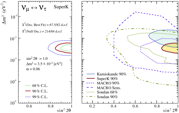
Figure 11: a (left): Allowed regions obtained by Super-K based upon $\chi^{2}$ fitting to FC and PC single ring events, plus upward stopping muons, plus upward through-going muons. b (right): Oscillation parameter allowed regions from Kamiokande (thin-line boundary), Super-K (thick-line boundary), MACRO (dashed boundaries), and Soudan 2 (dotted and dot-dashed boundaries).

In order to gauge the overall consistency of atmospheric neutrino observations, the various oscillation-parameter allowed regions obtained by each of the underground experiments have been assembled in Fig. 11b. Along with the 90% CL region from the Super-K all data fit discussed above, we include the final 90% CL region reported by Kamiokande (thin-line boundary) [23]. From MACRO, we show the 90% CL region and include the experimental sensitivity at 90% CL (dashed boundaries). For Soudan 2, we plot the region allowed at 68% and 90% CL. Fig. 11b shows that, for two independent water Cherenkov detectors and for two quite different tracking calorimeters, there is a region of oscillation parameter values which is acceptable to all experiments. Now “Fools rush in where Angels fear to tread”, it is often said. And concerning the significance of Fig. 11b the Angels will urge caution, for the atmospheric data show neutrino disappearance only - oscillation appearance has yet to be shown. Nevertheless, this Fool cannot resist the rush: I propose to you that congratulations are in order for the researchers of Kamiokande and of Super-K and more generally, for the non-accelerator underground physics community. For Fig. 11b, Ladies and Gentlemen, is the portrait of a Discovery - the discovery of neutrino oscillations with two-state mixing.

10 Dominant and Sub-Dominant Two-State Mixing

Assuming that muon neutrinos oscillate into other flavor(s), with nearly maximal mixing and with $\Delta m^{2}$ in the range $10^{-2}$ to $10^{-3}$ eV², it is of interest to consider what flavors are involved in the dominant two-state oscillation, and in other possible sub-dominant oscillations. That $\nu_{\mu}\rightarrow\nu_{e}$ could be the dominant mode for $\nu_{\mu}$ disappearance is ruled out by the CHOOZ reactor experiment. CHOOZ has established a limit on $\overline{\nu}_{e}$ disappearance [24]; by CPT symmetry, this limit implies that $\nu_{e}$ neutrinos do not disappear, or at least not in a parameter regime which is relevant to the atmospheric flux.

Since it is generally believed that $\nu_{\mu}\rightarrow\nu_{\tau}$ oscillation is the dominant mode, it is natural to ask: Where are the $\nu_{\tau}$ events? In the dominant $\nu_{\mu}\rightarrow\nu_{\tau}$ scenario, about 0.9 charged current $\nu_{\tau}$ events per kiloton year exposure can be expected to occur in an underground detector [25]. Then, in exposures reported at this Symposium, we would expect Super-K to have recorded $\approx 47$ FC or PC charged current $\nu_{\tau}$ events and Soudan 2 to have recorded about 4 events. These events will be up-going but otherwise indistinguishable from energetic NC events, and so there is little hope that $\nu_{\tau}$ reactions can be isolated by the on-going atmospheric neutrino experiments. It would be heartening to see a few unambiguous tau-neutrino interactions - even from an accelerator experiment! On this, hopes are placed with the $\nu_{\tau}$ candidates recorded by the DONUT hybrid emulsion experiment at Fermilab [26].

Although dominant $\nu_{\mu}\rightarrow\nu_{\tau}$ is unlikely to be confirmed anytime soon via $\nu_{\tau}$ appearance, progress has been made by Super-K towards eliminating the remaining competition which is $\nu_{\mu}\rightarrow\nu_{sterile}$ oscillations. Now sterile neutrinos, by definition, do not interact with normal matter via neutral currents, a fact which has consequences currently being examined by Super-K. Firstly, it follows that sterile neutrinos cannot produce single $\pi^{0}$ events since these are NC reactions: $\nu_{s}N\not\rightarrow\nu_{s}N\pi^{0}$. Then, relative to the $\nu_{\mu}\rightarrow\nu_{\tau}$ scenario, $\nu_{\mu}\rightarrow\nu_{s}$ will result in fewer single $\pi^{0}$ events, and the relative dearth of these final states will be in up-going directions [27]. Unfortunately, cross sections for these NC reactions have large uncertainties, a situation which hinders the isolation of a depletion which is demonstrably significant [28].

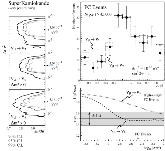
Figure 12: a (left): Allowed regions for $\nu_{\mu}\rightarrow\nu_{\tau}$ and for $\nu_{\mu}\rightarrow\nu_{sterile}$ two-state mixing scenarios, obtained from FC single ring events of Super-K. b (right,top): Zenith angle distribution for selected energetic PC events of Super-K (solid circles); histograms show the $\nu_{\mu}\rightarrow\nu_{\tau}$ and $\nu_{\mu}\rightarrow\nu_{s}$ solutions of Fig. 12a. c (right,bottom): Up/Down ratio versus log ($\Delta m^{2}$) for the energetic PC events. Curves depict predictions from $\nu_{\mu}\rightarrow\nu_{\tau}$ (dashed) and $\nu_{\mu}\rightarrow\nu_{s}$ (dotted) oscillation scenarios. The observed ratio $\pm 1\sigma$ defines the horizontal band allowed by the data.

More generally, the absence of coupling to the Z⁰ for sterile neutrinos means that their effective potential in matter differs from that for $\nu_{\mu}$ neutrinos. The difference in respective matter potentials can be written

$$V_{\mu}-V_{s}=\mp\sqrt{2}G_{F}\frac{N_{n}}{2},$$ (7)

where the difference is negative (positive) for neutrinos (antineutrinos) and $N_{n}$ is the neutron number density. For high energy $\nu_{\mu}$’s traversing matter, the existence of this potential difference causes $\nu_{\mu}\rightarrow\nu_{s}$ to be suppressed relative to $\nu_{\mu}\rightarrow\nu_{\tau}$ in a way that may be discernible [29, 30]. To elucidate the effect, the neutrinos of lower energy observed in Super-K can be used to establish a baseline for neutrino oscillation behavior. Fig. 12a shows allowed regions in the parameter plane obtained from three different oscillation fits to the FC single-ring events. The allowed region for $\nu_{\mu}\rightarrow\nu_{\tau}$ oscillations (Fig. 12a-top) is as described previously with (1.0, $3.0\times 10^{-3}$ eV²) as best values. For $\nu_{\mu}\rightarrow\nu_{s}$ there are two solutions with two allowed regions (Fig. 12a-middle, bottom); these arise from the two possibilities with the sign of the mass squared difference which occurs between mass eigenstates involved in the mixing. However the allowed regions are found to be very similar in all three cases, with fits of comparable quality, consequently $\nu_{\mu}\rightarrow\nu_{s}$ is practically indistinguishable from $\nu_{\mu}\rightarrow\nu_{\tau}$ for the FC events.

For higher energy neutrinos however this ‘degeneracy’ can be altered by matter traversal, a possibility which can be seen by examining oscillation phenomenology appropriate for neutrinos moving through matter of uniform density. Interestingly, matter effects for $\nu$ oscillations can be formulated in a way which is look-alike to phenomenology for vacuum oscillations [30, 31]. One feature is that the mixing angle for vacuum oscillations $\sin^{2}2\theta$ goes over to $\sin^{2}2\theta_{m}$ for oscillations in matter

$$\sin^{2}2\theta_{m}=\frac{\sin^{2}2\theta}{\sin^{2}2\theta+(D-\cos 2\theta)^{2}},$$ (8)

where $D$ is proportional to $E_{\nu}$ and to the difference in effective potentials in matter for the mixing neutrino flavors

$$D=\frac{2E_{\nu}V_{\alpha\beta}}{\Delta m^{2}}\mbox{ }\mbox{ where }V_{\alpha\beta}\equiv V_{\alpha}-V_{\beta}.$$ (9)

For $\nu_{\mu}\rightarrow\nu_{\tau}$, $V_{\mu\tau}=0$ and hence $D=0$, consequently matter traversal produces no effect on this oscillation. For $\nu_{\mu}\rightarrow\nu_{s}$ however, and for $\nu_{\mu}\rightarrow\nu_{e}$ as well, $V_{\mu s}$ ($V_{\mu e}$) is non-zero, and is in fact sign-dependent since anti-neutrinos are affected differently than are neutrinos. Then $D$ is non-zero and acquires a sizable magnitude at high $E_{\nu}$. Because of its occurrence in the denominator of $\sin^{2}2\theta_{m}$, it acts to suppress $\nu_{\mu}\rightarrow\nu_{s}$ at high energies, a suppression which is absent for $\nu_{\mu}\rightarrow\nu_{\tau}$.

To test for occurrence of matter-induced oscillation suppression, SuperKamiokande has examined two different high energy neutrino samples. The first sample consists of PC events for which the number of photo-electrons from each event exceeds 45,000. This is equivalent to requiring that $E_{vis}>5$ GeV; the sample thus obtained has $<E_{\nu}>\sim 25$ GeV. The zenith angle distribution for these events is shown in Fig. 12b. The data (solid circles) are binned in $\cos\theta_{z}$ from -1.0 to 1.0. Shown superposed are the predictions [30] from $\nu_{\mu}\rightarrow\nu_{\tau}$ and for $\nu_{\mu}\rightarrow\nu_{s}$, with $\Delta m^{2}$ and $\sin^{2}2\theta$ set to the values inferred from the FC events. A difference between these distributions is apparent for $\cos\theta_{z}$ below -0.2. Neutrinos which initiate events in this region travel thousands of kilometers through the Earth, and thus experience matter effects. For the $\nu_{sterile}$ oscillation case, matter effects suppress the $\nu_{\mu}\rightarrow\nu_{s}$ oscillation, consequently fewer $\nu_{\mu}$’s “disappear”. The expectation therefore lies above the curve for $\nu_{\mu}\rightarrow\nu_{\tau}$. Interestingly, it also lies above the data.

To quantify the difference, an up-down ratio is used. Here, the number of $\nu_{\mu}$’s which are upward-going (and consequently subject to matter suppression for the $\nu_{\mu}\rightarrow\nu_{s}$ case) is compared to the downward-going flux which, at high energies, is not affected by oscillations: $(N_{up}(\cos\theta<-0.4)/N_{down}(\cos\theta>+0.4))_{DATA}=0.50\pm 0.12\pm 0.01.$ In comparison, the ratio $N_{up}/N_{down}$ is is $0.94\pm 0.04$ from the null oscillation MC. Assuming $\sin^{2}2\theta=1.0$, this ratio can be plotted versus $\Delta m^{2}$ as in Fig. 12c. The region allowed by the data corresponds to the horizontal band centered at $N_{up}/N_{down}=0.50$ with boundaries at $\pm 1\sigma$. Curves obtained from the $\nu_{\mu}\rightarrow\nu_{\tau}$ and $\nu_{\mu}\rightarrow\nu_{s}$ scenarios are also drawn. For $\nu_{\mu}\rightarrow\nu_{\tau}$, the predicted curve falls within the band allowed by the data for plausible values of $\Delta m^{2}$ which include the best fit value obtained with the FC events. For $\nu_{\mu}\rightarrow\nu_{s}$ however, the scenario curve lies above the allowed band, only “entering” at a $\Delta m^{2}$ which is higher than the FC best fit value.

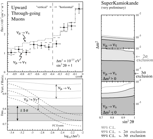
Figure 13: a (left,top): Flux of upward through-going muons versus $\cos\theta_{z}$ in Super-K. The histograms depict $\nu_{\mu}\rightarrow\nu_{\tau}$ and $\nu_{\mu}\rightarrow\nu_{s}$ solutions. b (left,bottom): Vertical/Horizontal ratio versus $\log(\Delta m^{2})$ for muons of 13a, with predictions from $\nu_{\mu}\rightarrow\nu_{\tau}$ (dashed band) and $\nu_{\mu}\rightarrow\nu_{s}$ (dotted band) oscillation scenarios. c (right): Exclusion regions for $\nu_{\mu}\rightarrow\nu_{\tau}$ and $\nu_{\mu}\rightarrow\nu_{s}$ scenarios obtained by fitting to Up/Down and Vertical/Horizontal ratios from energetic PC and through-going muon samples, to be compared to the allowed regions of Fig. 12a.

A similar pattern is found with zenith angles for upward through-going muons in Super-K, a sample for which $<E_{\nu}>$ $\simeq~{}100$ GeV. Figure 13a shows the $\cos\theta_{z}$ distribution of that sample, with $\nu_{\mu}\rightarrow\nu_{\tau}$ and for $\nu_{\mu}\rightarrow\nu_{s}$ shown superposed. As observed with energetic PCs, matter suppression for $\nu_{\mu}\rightarrow\nu_{s}$ places the prediction (at $\sin^{2}2\theta$, $\Delta m^{2}$ from the FC events) above the data for angles of incidence corresponding to large path lengths through the Earth. To quantify the differences in scenarios here, the data distribution is separated into “horizontal” ($\cos\theta>-0.4$) and “vertical” ($\cos\theta<-0.4$) events and the vertical to horizontal ratio is calculated: $(N_{vertical}/N_{horizontal})_{DATA}=0.77\pm 0.05\pm 0.01.$ As shown in Fig. 13b, there is no value of $\Delta m^{2}$ for which the $\nu_{\mu}\rightarrow\nu_{s}$ scenarios predict $N_{v}/N_{h}$ in the value range indicated by the through-going muon data.

The difference between data and MC predictions for the three oscillations scenarios can be evaluated using a chi-square function $\chi^{2}=\chi^{2}_{PC}+\chi^{2}_{thru-\mu}$ where $\chi^{2}_{PC}$ contains the difference for the up/down ratio and $\chi^{2}_{thru-\mu}$ the difference for the vertical/horizontal ratio. Parameter regions excluded at 90% and 99% CL are then deduced from $\chi^{2}$, corresponding approximately to 2$\sigma$ and 3$\sigma$ exclusion. The exclusion regions for each of the three oscillation scenarios are displayed as shaded areas in Fig. 13c. Comparison of these excluded regions with the oscillation-allowed regions of Fig. 12a, shows large portions of $\nu_{\mu}\rightarrow\nu_{s}$, for both $\Delta m^{2}>$ 0 and $<$ 0, to be excluded at the 2$\sigma$ level. While the observations do not as yet rule out $\nu_{\mu}\rightarrow\nu_{s}$, it is clear that this new approach by Super-K can be steadily strengthened with more exposure.

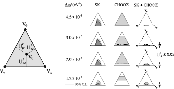
Figure 14: a (left): Triangle graph for displaying possible flavor compositions of the mass eigenstate $\nu_{3}$. b (right) Regions of allowed ($U^{2}_{e3}$, $U^{2}_{\mu 3}$, $U^{2}_{\tau 3}$) versus $\Delta m^{2}$, obtained by fitting the Super-K and CHOOZ data via three-flavor mixing in the approximation of one mass scale dominance [32].

11 Subdominant $\nu_{\mu}\leftrightarrow\nu_{e}$ in Three-Flavor Mixing

For a view of possibilities with subdominant oscillations, we turn to investigations of three-flavor mixing. A number of approaches have been discussed in the literature [32]. Here we review a scenario for subdominant $\nu_{\mu}\rightarrow\nu_{e}$ which emerges directly from the approximation of one mass scale dominance. In this approximation it is assumed that one of the mass eigenstates - $\nu_{3}$ let us say - is more massive than the other two, and that the lighter $\nu_{1,2}$ eigenstates are nearly mass-degenerate. As a result there are two mass-squares differences $\Delta m^{2}=|m_{3}^{2}-m_{1,2}^{2}|$ and $\delta m^{2}=|m_{2}^{2}-m_{1}^{2}|$ having different magnitudes. The larger $\Delta m^{2}$ can be identified with the dominant two-state mixing observed with atmospheric oscillations, whereas the much smaller $\delta m^{2}$ relates to oscillations not observable with atmospheric $\nu$’s but presumably relevant to solar $\nu$’s. Up to terms of order $(\delta m^{2})/(\Delta m^{2})$ the parameter space for atmospheric neutrinos is spanned by $(\Delta m^{2},U_{e3}^{2},U_{\mu 3}^{2},U_{\tau 3}^{2})$. The amplitudes satisfy the unitary constraint $U_{e3}^{2}+U_{\mu 3}^{2}+U_{\tau 3}^{2}=1$.

For vacuum oscillations, it follows that the oscillation probability for transitions between flavors $\alpha$ and $\beta$ is

$$P^{vac}(\nu_{\alpha}\leftrightarrow\nu_{\beta})=4\mbox{ }U^{2}_{\alpha 3}\cdot U^{2}_{\beta 3}\cdot\sin^{2}\left[\frac{1.27\mbox{ }\Delta m^{2}\cdot L}{E_{\nu}}\right].$$ (10)

As suggested by the amplitudes in this expression, the flavor composition of the massive $\nu_{3}$ eigenstate is the central issue:

$$\nu_{3}=U_{e3}\cdot\nu_{e}+U_{\mu 3}\cdot\nu_{\mu}+U_{\tau 3}\cdot\nu_{\tau}.$$ (11)

For fixed $\Delta m^{2}$, the $\nu_{3}$ composition is conveniently depicted using the equilateral triangle construction shown in Fig. 14a for which the unitarity constraint is automatically incorporated.

Fogli, Lisi, Marrone, and Scioscia have compared predictions for specific choices of $(\Delta m^{2},U_{e3}^{2},U_{\mu 3}^{2},U_{\tau 3}^{2})$ with Super-K zenith angle distributions; the constraint on $\nu_{e}\rightarrow\nu_{\mu}$ from the CHOOZ limit has also been included. They find that two-flavor oscillations with maximal $\nu_{\mu}\leftrightarrow\nu_{\tau}$ mixing works rather well [32]:

$$\sin^{2}2\theta_{\mu\tau}=4\mbox{ }U_{\mu 3}^{2}\cdot U_{\tau 3}^{2}\simeq 1.0\mbox{ }\mbox{ with }\mbox{ }U_{\mu 3}^{2}\simeq U_{\tau 3}^{2}\simeq 1/2\mbox{ }\mbox{ and }\mbox{ }U_{e3}^{2}\simeq 0.$$ (12)

A small admixture of $U_{e3}^{2}$ is however allowed by the fits to data as is shown graphically in Fig. 14b. Here, for a relevant selection of $\Delta m^{2}$ values, the domain of $U_{f3}^{2}$ values allowed by Super-K data at 90 and 99% CL comprise the shaded areas in the triangle graphs of the left-most column. Elimination of regions excluded by CHOOZ (see center-column triangle graphs) leaves the diminished but still existent allowed regions shown in the right-most column of Fig. 14b. From the height of the various allowed regions, it is concluded that $U_{e3}^{2}\stackrel{{\scriptstyle<}}{{\sim}}0.05$. The expression for the $(\nu_{\mu}\rightarrow\nu_{e})$ vacuum oscillation probability follows immediately from Eq. (10) with $\alpha$, $\beta$ assigned to $\mu$, $e$ respectively. We infer from this formula that $P^{vac}(\nu_{\mu}\rightarrow\nu_{e})$ can be as large as 0.10.

12 $P(\nu_{\mu}\rightarrow\nu_{e})$ Amplification via Matter Resonances

A $\nu_{\mu}\leftrightarrow\nu_{e}$ oscillation of strength as indicated above will be hard to discern within the atmospheric flux, however we may get some help, as a result of amplification by matter resonances in the Earth. Two kinds of resonance effects are possible.

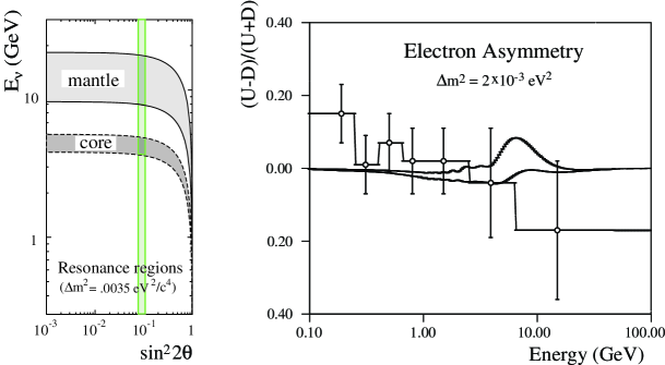
Figure 15: a (left): Values of $\sin^{2}2\theta$ and $E_{\nu}$ for which $\nu_{\mu}$ to $\nu_{e}$ mixing of atmospheric neutrinos could be enhanced by MSW resonance in the Earth’s mantle or core [33]. b (right): Possible “bump” in up/down asymmetry of $\nu_{e}$ flavor neutrinos which could arise with MSW resonant enhancement in the Earth’s mantle [34].

One arises with the MSW resonance wherein the $D$ of Eq. (9) containing $V_{e\mu}$ approximates $\cos^{2}2\theta$ with the consequence that $\sin^{2}2\theta_{m}\simeq 1.0$. Depending upon the particular values of the mixing parameters, MSW enhancement can take place either in the terrestrial mantle or core for the $E_{\nu}$ intervals depicted in Fig. 15a [33]. An MSW resonance could result in a bump in the upward-going $\nu_{e}$ flux at the resonance energy. This possibility has been examined by J. Pantaleone who proposes that the $\nu_{e}$ up-down asymmetry could be a useful discriminant, with possible outcome as illustrated in Fig. 15b [34]. Of interest to long baseline experiments, e.g. K2K and MINOS, is the observation that MSW enhancement can also take place in the Earth’s crust [35].

A second and different resonance-like enhancement can take place for atmospheric neutrinos which cross the Earth’s core. For such neutrinos, having paths that cross the mantle, the core, and again the mantle, a complex constructive interference among the oscillation amplitudes arising in regions of different density is possible. The algebraic delineation of this effect has been presented by M.V. Chizhov and S.T. Petcov [36]. Their work has yielded striking depictions of the transition probabilities as shown in Fig. 16. (Alternative formulations and interpretations have been presented; see Refs. [37].)

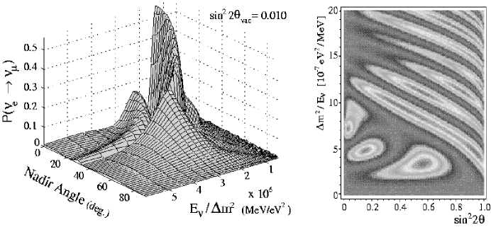
Figure 16: a (left): The probability P($\nu_{e(\mu)}\rightarrow\nu_{\mu;\tau(e)}$) for atmospheric neutrinos with mantle-core-mantle trajectories through the Earth. Such neutrinos may undergo a resonance-like enhancement (the large peak) which is different from an MSW enhancement. b (right): Regions of resonance-like enhancement for Earth core-crossing neutrinos [36].

Fig. 16a shows $\nu_{e}\leftrightarrow\nu_{\mu}$ oscillation probability as a function of nadir angle (neutrinos at vertically upward incidence being at $0^{0}$) and of $E_{\nu}/\Delta m^{2}$ in units of (MeV/eV²). Here the smaller peak at $E_{\nu}/\Delta m^{2}=2.5\times 10^{6}$ is the MSW resonance in the Earth’s mantle. The distinctly larger structure arises with the mantle-core-mantle trajectories. The structures shown in Fig. 16a are to be found on the “probability island” at lowest $\sin^{2}2\theta$ in Fig. 16b. Other resonance structures exist at higher mixing angle values as shown.

In the on-going underground experiments the effective integrations over $E_{\nu}$, $\cos\theta_{z}$, and detector resolution effects, which necessarily occur with the accumulation of data events, likely assure that matter resonance effects will be difficult to observe. Be that as it may, these are intriguing phenomena, underwritten by phenomenology which is rich and well-grounded. Their elucidation poses an interesting challenge for a neutrino factory to be built at a muon collider [33, 38].

13 Atmospheric Fluxes; Concluding Remarks

Invaluable to all oscillation analyses with atmospheric neutrinos are developments which yield improved knowledge in rates and shapes of atmospheric flux spectra. There have been several such developments of recent, which we briefly remark upon here. Firstly there is the observation by Super-K of the east-west anisotropy in horizontal neutrino fluxes at the Kamioka site [40]. The $\nu_{\mu}$ and $\nu_{e}$ fluxes from the east are found to be depleted, as expected due to geomagnetic cutoff of charged cosmic ray primaries and as calculated in the one-dimensional models of the atmospheric cascade [41]. Just arrived “on the scene”, are three-dimensional atmospheric flux calculations which have been prepared independently by two groups [42]. Their arrival is timely indeed, since 3-D calculations are the natural framework in which to utilize the abundant data becoming available from balloon-borne spectrometer experiments. These experiments measure the primary cosmic ray flux and sample the secondary muon fluxes at a variety of depths in the atmosphere [43].

Concerning flux-related measurements, there are “swords-in-the-stone” aplenty to tantalize the brave-of-heart. For example, no experiment to date has separated and compared the atmospheric anti-neutrino fluxes to the neutrino fluxes. It is within the capability of the underground experiments to distinguish $\overline{\nu}_{\mu}$ from $\nu_{\mu}$ interactions [44], and the $\nu$, $\overline{\nu}$ reaction cross sections are known. Nevertheless, the assertion by all of the flux calculations that the ratio of $\Phi(\overline{\nu})$ to $\Phi(\nu)$ is very nearly 1:1 for either atmospheric neutrino flavor, remains untested. To this end, a $\overline{\nu}_{\mu}$/$\nu_{\mu}$ ratio of ratios measurement would be interesting [45]. As a second example, we note the absence of measurements which examine variations in the atmospheric neutrino fluxes predicted to occur as a function of the solar cycle. The variations are substantial in the sub-GeV portion of $E_{\nu}$ spectra and should be more pronounced at northern geomagnetic latitudes [46]. Such a measurement of course places a premium on continuous exposures which extend to a decade or longer; however IMB, Kamiokande, and Soudan 2 have shown solar-cycle-duration exposures to be attainable.

To conclude: A bonanza in neutrino oscillations research is in progress, driven to fever pitch by recent experimental observations with atmospheric neutrinos. Quite possibly, the finest nuggets are still in the ground. Fortunately the atmospheric beam is always on and beamline access is free; however the detectors required for future progress will not materialize cheaply [47]. In any case, the aura of adventure and discovery which now pervades the atmospheric neutrino beamline will remain for some time. The Dreamers and the Restless will come to try their luck, and among them - appearance probability of 1.0 - will be participants from this Symposium.

It is a pleasure to thank the organizers of the Symposium, and especially Helen Quinn and John Jaros, for the opportunity to give this Talk. I am greatly indebted to Takaaki Kajita, Serguey Petcov, Ed Kearns, John Learned, Francesco Ronga, Maurizio Spurio, Tomas Kafka, Jack Schneps, Maury Goodman, and Sandip Pakvasa for communications and discussion relating to physics with atmospheric neutrinos.

Discussion

B.F.L. Ward (University of Tennessee): How do we combine the results for $\Delta m^{2}$ from SuperKamiokande and for Soudan 2, for example $3.5\times 10^{-3}$ eV² and $8\times 10^{-3}$ eV² ?

Reply: I would not recommend doing that. The Soudan 2 and MACRO measurements are interesting as checks, with completely different technique and systematics, on the Super-K result. But since the three determinations are in agreement and since the Super-K measurement is the one with predominant statistical weight, the Super-K value is the one to be used.

Peter Rosen (DOE): The evidence for oscillations from atmospheric neutrinos is certainly impressive and the community of non-accelerator physicists is certainly to be congratulated. To what extent can you rule out alternative explanations? For example, Vernon Barger, Sandip Pakvasa et al. have shown that the data can be fitted by a neutrino decay scenario.

Reply: The work to which you refer [48] makes a good case for neutrino decay being viable as an alternative to neutrino oscillations. Also, there are other explanations, e.g. flavor changing neutrino interactions, which are not ruled out [49].

S. Ragazzi (University of Milano): What do you expect to learn from the comparison of $\Phi(\overline{\nu})$ and $\Phi(\nu)$ ?

Reply: The atmospheric neutrino flux calculations predict anti-neutrino fluxes to be nearly the same as neutrino fluxes; this should be tested. Although no difference is to be expected from the viewpoint of conventional flavor oscillations, I note that neutrino into anti-neutrino oscillation schemes have good lineage, originating with Pontecorvo’s proposal of 1957 [50].

Jasper Kirkby (CERN): Have you looked in your data for a signal of $\gamma$’s produced by solar cosmic rays? These are produced by events lasting a few days and created by energetic coronal mass ejections from the sun. They produce particles with peak energies of about 100 MeV, and occasionally up to about 1 GeV. During the most energetic events a large ionization—equivalent to 20-30% of the total annual galactic cosmic ray flux—is dumped into the Earth’s atmosphere. These events occur near solar maximum, which we are entering now. I would guess Super-K may be able to detect $\nu$’s in-time with these events. Perhaps they could even contribute to the distortion of the solar neutrino energy spectrum we saw in the previous talk in the hep $\nu$ energy region.

Chang-Kee Jung (SUNY, Stony Brook): SuperKamiokande has examined data for solar activity dependence for long-term periods. But we have not done so for specific short period dependence on solar flares.

References

- [1]
- [2] D. Ayres et al., Phys. Rev. D 29, 902 (1984).
- [3] P. Fisher, B. Kayser, and K.S. McFarland, to appear in Annu. Rev. Nucl. Part. Sci., hep-ph/9906244.
- [4] T. Kajita (SuperKamiokande), Nucl. Phys. B Proc. Suppl. 77, 123 (1999); K. Scholberg, in Proceedings of the Int. Workshop on Neutrino Telescopes, edited by M. Baldo Ceolin, Venice, Italy, February 1999, hep-ex/9905016.
- [5] S. Ahlen et al. (MACRO), Nucl. Inst. Meth. A 324, 337 (1993).
- [6] M. Ambrosio et al. (MACRO), Astropart. Phys. 9, 105 (1998).
- [7] W.W.M. Allison et al. (Soudan 2), Nucl. Instr. Meth. A 376, 36 (1996); A 381, 385 (1996); W.P. Oliver et al., Nucl. Instr. Meth. A 275, 371 (1989).
- [8] Y. Fukuda et al. (SuperKamiokande), Phys. Lett. B 433, 9 (1998); Phys. Rev. Lett. 81, 1562 (1998); Phys. Lett. B 436, 33 (1998).
- [9] W.W.M. Allison et al. (Soudan 2), Phys. Lett. B 391, 491 (1997); Phys. Lett. B 449, 137 (1999).
- [10] K.S. Hirata et al. (Kamiokande), Phys. Lett. B 205, 416 (1988); Phys. Lett. B 280, 146 (1992); Y. Fukuda et al., Phys. Lett. B 335, 237 (1994).
- [11] D. Casper et al. (IMB-3), Phys. Rev. Lett. 66, 2561 (1991); R. Becker-Szendy et al., Phys. Rev. D 46, 3720 (1992).
- [12] M. Aglietta et al. (NUSEX), Europhys. Lett. 8, 611 (1989).
- [13] Ch. Berger et al. (Fréjus), Phys. Lett. B 227, 489 (1989); Phys. Lett. B 245, 305 (1990); K. Daum et al., Z. Phys. C 66, 417 (1995).
- [14] This figure is an updated version of Fig. 1 in P.F. Harrison, D.H. Perkins, and W.G. Scott, Phys. Lett. B 396, 186 (1997).
- [15] V.J. Stenger, Proceedings of Snowmass ’94, Particle and Nuclear Astrophysics and Cosmology in the Next Millenium, Snowmass, Colorado, June 29 - July 14, 1994, p. 167.
- [16] M. Honda et al., Phys. Lett. B 248, 193 (1990); M. Honda et al., Phys. Rev. D 52, 4985 (1995).
- [17] H. Gallagher (Soudan 2), in Proceedings of the 29th Int. Conf. on High Energy Physics, Vancouver, edited by A. Astbury, D. Axen, and J. Robinson, (World Scientific, Singapore, 1999); W.A. Mann, T. Kafka, and M. Sanchez, in Proceedings of the Int. Workshop on Neutrino Telescopes, edited by M. Baldo Ceolin, Venice, Italy, February 1999.
- [18] T.K. Gaisser, T. Stanev, and G. Barr, Phys. Rev. D 38, 85 (1988); G. Barr, T.K. Gaisser, and T. Stanev, Phys, Rev. D 39, 3532 (1989). An improved calculation is reported in V. Agrawal, T.K. Gaisser, P. Lipari, and T. Stanev, Phys. Rev. D53, 1313 (1996).
- [19] A. Surdo (MACRO), hep-ex/9905028; M. Spurio, hep-ex/9908066.
- [20] Y. Fukuda et al. (SuperKamiokande), Phys. Rev. Lett. 82, 2644 (1999); Y. Fukuda et al., submitted to Physics Letters, hep-ex/9908049.
- [21] S. Ahlen et al. (MACRO), Phys. Lett. B 357, 481 (1995); M. Ambrosio et al., Phys. Lett. B 434, 451 (1998); F. Ronga, hep-ex/9905025.
- [22] G.J. Feldman and R.D. Cousins, Phys. Rev. D 57, 3873 (1998).
- [23] S. Hatakeyama et al. (Kamiokande), Phys. Rev. Lett. 81, 2016 (1998).
- [24] M. Apollonio et al. (CHOOZ), Phys. Lett. B 420, 397 (1998); M. Apollonio et al., hep-ex/9907037.
- [25] M.D. Messier (SuperKamiokande), PhD Thesis, Boston University (1999).
- [26] T. Kafka (DONUT), Nucl. Phys. B Proc. Suppl. 70, 204 (1999); http://fn872.fnal.gov.
- [27] J.G. Learned, S. Pakvasa, and J.L. Stone, Phys. Lett. B 435, 131 (1998).
- [28] F. Vissani and A.Yu. Smirnov, Phys. Lett. B 432, 376 (1998); A. Geiser, Eur. Phys. J. C7, 437 (1999).
- [29] Q.Y. Liu and A.Yu. Smirnov, Nucl. Phys. B 524, 505 (1998); Q.Y. Liu, S.P. Mikheyev, and A.Yu. Smirnov, Phys. Lett. B 440, 319 (1998); R. Foot, R.R. Volkas, and O. Yasuda, Phys. Rev. D 58, 013006 (1998); O. Yasuda, Nucl. Phys. B Proc. Suppl. 77, 146 (1999), hep-ph/9809206.
- [30] P. Lipari and M. Lusignoli, Phys. Rev. D 58, 073005 (1998).
- [31] S.P. Rosen in “Los Alamos Science: Celebrating the Neutrino”, LAUR 97-2534, 164 (1997).
- [32] G.L. Fogli, E. Lisi, A. Marrone, and G. Scioscia, Phys. Rev. D 59, 033001 (1998); G.L. Fogli et al., hep-ph/9904465; O. Yasuda, Phys. Rev. D 58, 091301 (1998); V. Barger and K. Whisnant, Phys. Rev. D 59, 093007 (1999); T. Sakai and T. Teshima, hep-ph/9901219; O.L.G. Peres and A.Yu. Smirnov, Phys. Lett. B 456, 204 (1999).
- [33] V. Barger, S. Geer, and K. Whisnant, hep-ph/9906487.
- [34] J. Pantaleone, Phys. Rev. Lett. 81, 5060 (1998); see also G. Barenboim and F. Scheck, Phys. Lett. B 450, 189 (1999).
- [35] P. Lipari, hep-ph/9903481; M. Narayan and S. Uma Sankar, hep-ph/9904302.
- [36] S.T. Petcov, Phys. Lett B 434, 321 (1998); 444, 584(E) (1998); S.T. Petcov, Nucl. Phys. Proc. Suppl. 77, 93 (1999), hep-ph/9809587; M.V. Chizhov, M. Maris, and S.T. Petcov, Report No. SISSA 53/98/EP, 1998, hep-ph/9810501; M.V. Chizhov and S.T. Petcov, hep-ph/9903424; S.T. Petcov, to appear in Proceedings of the Int. Workshop on Weak Interactions and Neutrinos, Jan. 25-30, 1999, Cape Town, South Africa, hep-ph/9907216; M.V. Chizhov and S.T. Petcov, Phys. Rev. Lett. 83, 1096 (1999).
- [37] E.Kh. Akhmedov, Nucl. Phys. B 538, 25 (1999); E.Kh. Akhmedov, A. Dighe, P. Lipari, and A.Yu. Smirnov, Nucl. Phys. B 542, 3 (1999); E.Kh. Akhmedov, hep-ph/9903302; J. Pruet and G.M. Fuller astro-ph/9904023.
- [38] M. Campanelli, A. Bueno, and A. Rubbia, hep-ph/9905240.
- [39] T.K. Gaisser, M. Honda, K. Kasahara, H. Lee, S. Midorikawa, V. Naumov, and T. Stanev, Phys. Rev. D 54, 5578 (1996); T.K. Gaisser, Nucl. Phys. Proc. Suppl. 77, 133 (1999); M. Honda, Nucl. Phys. Proc. Suppl. 77, 140 (1999).
- [40] T. Futagami et al. (SuperKamiokande), Phys. Rev. Lett. 82, 5194 (1999).
- [41] P. Lipari, T. Stanev, and T.K. Gaisser, Phys. Rev. D 58, 073003 (1998).
- [42] G. Battistoni, A. Ferrari, P. Lipari, T. Montaruli, P.R. Sala, and T. Rancati, hep-ph/9907408; Y. Tserkovnyak, R. Tomar, C. Nally, and C. Waltham, hep-ph/9907450.
- [43] M. Boezio et al. (CAPRICE94), Phys. Rev. Lett. 82, 4757 (1999); R. Bellotti et al. (MASS), Phys. Rev. D 60, 052002 (1999).
- [44] J.M. LoSecco, Phys. Rev. D 59, 117302 (1999).
- [45] F. Vannucci, CERN/SPSC 98-26, SPSC/M613 Report (1998).
- [46] P. Lipari, in Proceedings of the Int. Workshop on Neutrino Telescopes, edited by M. Baldo Ceolin, Venice, Italy, February 1999, hep-ph/9905506.
- [47] M. Aglietta et al., hep-ex/9907024; M. Campanelli et al., hep-ex/9905035; J. Panman, in Proceedings of the Int. Workshop on Neutrino Telescopes, edited by M. Baldo Ceolin, Venice, Italy, February 1999; J.G. Learned and T. Ypsilantis, Univ. of Hawaii technical note.
- [48] V. Barger, J.G. Learned, P. Lipari, M. Lusignoli, S. Pakvasa, and T.J. Weiler, hep-ph/9907421.
- [49] For discussion and references, see S. Pakvasa, hep-ph/9910246.
- [50] See S.M. Bilenky, hep-ph/9908335.