A Proposal for a Different Chi-square Function for Poisson Distributions

Abstract

We obtain an approximate Gaussian distribution from a Poisson distribution after doing a change of variable. A new chi-square function is obtained which can be used for parameter estimations and goodness-of-fit testing when adjusting curves to histograms. Since the new distribution is approximately Gaussian we can use it even when the bin contents are small. The corresponding chi-square function can be used for curve fitting. This chi-square function is simple to implement and presents a fast convergence of the parameters to the correct value, especially for the parameters associated with the width of the fitted curve. We present a Monte Carlo comparative study of the fitting method introduced here and two other methods for three types of curves: Gaussian, Breit-Wigner and Moyal, when each bin content obeys a Poisson distribution. It is also shown that the new method and the other two converge to the same result when the number of events increases.

1 Introduction

Nowadays there is an intensive experimental effort to search for new phenomena in many fields of particle physics. These signals should be rare events where one needs to treat low statistics data and non-Gaussian errors. In order to handle these data one needs special care, since all the usual Gaussian procedures and techniques are no longer valid. On the other hand, it turns out that the minimization of the chi-square functions is normally simple, relatively fast and a very familiar way of fitting data, estimating parameters and their errors so as the goodness-of-fit testing. The $\chi^{2}$ of fitting a theoretical curve to experimental data in order to estimate some parameter values is to minimize the function

$$\chi^{2}_{G}=\sum_{i=1}^{N}\frac{(f(x_{i},\vec{\alpha})-n_{i})^{2}}{\sigma_{i}^{2}}$$ (1)

where $f(x_{i},\vec{\alpha})$ is a known function(model prediction) calculated at the point $x_{i}$ and $\vec{\alpha}$ is a vector of the parameters one wants to obtain; $n_{i}$ is the measured experimental value associated with the bin located at $x_{i}$ and $N$ is the number of bins in the range of interest. This method has been largely used but presents some limitations such as the assumption that each bin content must obey a Gaussian distribution of spread $\sigma_{i}$ or the measurement errors are at least almost ”Gaussian”. If the contents of each bin obeys a Poisson distribution some authors [1] recommend that each bin content must have at least a statistically significant number of entries $n_{i}$ such as that $\sigma_{i}\approx\sqrt{n_{i}}$, where the asymptotically limiting case for large number of measurements starts, and the square root of the variance can be considered as a good interval estimation. For values smaller than these, there are suggestions that one must use bins of variable sizes such that each bin content be greater than the statistically significant number of entries $n_{i}$. The disadvantage of these suggestions is that one can lose important information about the structure of the studied distribution. There is no rule of thumb for the bin width or for the ideal number of bins in which the region of interest should be divided. There is yet another hint that the ideal case is to use bins of variable width of equal probability contents [2].

In a very interesting paper, Baker and Cousins[3], call attention and discuss some topics such as point estimation, confidence interval estimation, goodness-of-fit testing, biased estimation, etc. when fitting curves to histograms using chi-square function.

They presented a $\chi^{2}_{BC}$ function for fitting histograms when the bin contents obey a Poisson distribution. They defined a Poisson likelihood chi-square which is given by Eq.(2) below,

$$\chi^{2}_{BC}=2\sum_{i=1}^{N}\left[f(x_{i},\vec{\alpha})-n_{i}+n_{i}log\left(n_{i}/f(x_{i},\vec{\alpha})\right)\right]$$ (2)

This function behaves asymptotically as a chi-square distribution and then can be used for estimation and goodness-of-fit testing.

The chi-function presented in this paper has also asymptotically a behavior like the classical chi-square function, a fast convergence to the correct value, much less fluctuations when compared with $\chi^{2}_{G}$ and it works also when one has distributions with long tails where bin contents can be very low. It is of easy implementation in any minimization program.

After this introduction, we demonstrate in section 2 how one can transform a non-Gaussian pdf into an approximate Gaussian pdf. Section 3 is devoted to obtain the chi-square function for the approximate Gaussian pdf from a Poisson distribution and discuss some of its characteristics. The next section, 4, we compare with the results obtained using the Eq.(1) and Eq.(2), and the new chi-square function for different number of entries in the histograms. This comparison is made using Monte Carlo events generated according to some distributions with known parameters, as suggested by [3] and in section 5 we present the conclusions. In the appendix we obtain the equivalent chi-square expression for a binomial distribution.

2 Obtaining an approximate Gaussian distribution

The basic motivation is to transform, via a variable transformation, a non-Gaussian probability density function(pdf) into an approximately Gaussian pdf preserving the probability even when one has small number of events [2, 4]. Let us consider a non-Gaussian pdf $p(x)$ and one wants to obtain a transformation such that the probability is preserved Eq.(3) and that the new pdf $q(z)$ should be approximately Gaussian:

$$q(z)dz=p(x)dx$$ (3)

Then $q(z)$ can be written as

$$q(z)=p(x)\left\arrowvert\frac{dx}{dz}\right\arrowvert$$ (4)

When a pdf is unimodal and obeys some regularity conditions [4], the logarithm of it is approximately quadratic so that

$$log(p(x))\approx log(p(\hat{x}))-\frac{1}{2}\left(-\frac{\partial^{2}log(p(x))}{\partial x^{2}}\right)_{\hat{x}}(x-\hat{x})^{2}$$ (5)

where $\hat{x}$ is the point associated to the maximum of $p(x)$ and one can define the following quantity

$$J(\hat{x})=\left(-\frac{\partial^{2}log(p(x))}{\partial x^{2}}\right)_{\hat{x}}$$ (6)

On the other hand, the logarithm of a Normal pdf $g(x)$, with mean $\hat{\mu}$ and standard deviation $\sigma$, is of the form:

$$log(g(x))=const-\frac{1}{2\sigma^{2}}(x-\hat{\mu})^{2}$$ (7)

so that given the location parameter $\hat{\mu}$, it is completely determined by its standard deviation $\sigma$.

A comparison between Eq.(5) and Eq.(7) shows that the variance of the pdf $p(x)$ is approximately equal to $J^{-1}(\hat{x})$. Let us suppose now that $z(x)$ is a one-to-one transformation between $x$ and $z$, then using the chain rule for derivatives one gets the relation

$$J(\hat{z}) = \left(-\frac{\partial^{2}log(p(x))}{\partial x^{2}}\right)_{\hat{x}}\left\arrowvert\frac{dx}{dz}\right\arrowvert^{2}_{\hat{z}}$$ (8)

$$= J(\hat{x})\left\arrowvert\frac{dx}{dz}\right\arrowvert^{2}_{\hat{z}}$$ (9)

Let us choose $z(x)$ such that

$$\left(\frac{dx}{dz}\right)_{\hat{z}}=J^{-1/2}(\hat{x})$$ (10)

This choice is made so as to make $J(\hat{z})$ independent of $\hat{z}$, the standard deviation equal to one and the new distribution $q(z)$ approximately translation invariant along the $z$ axis. Thus the metric can be obtained from the relationship obeying the above conditions

$$\frac{dz}{dx}=J^{1/2}(x)$$ (11)

$$z=\int^{x}J^{1/2}(t)dt$$ (12)

3 The Chi-square Function

As an example, let us apply the above prescription to a Poisson pdf given by

$$p_{P}(x)=\frac{x^{k}e^{-x}}{\Gamma(k+1)}$$ (13)

which means that after observing $k$ events one has a pdf of the estimated mean parameter $x$. Now one wants to find a Gaussian like pdf through a transformation of $x$. The location of the $p_{P}(x)$ maximum is easily shown to be at $\hat{x}=k$ and the term associated to the second derivative is

$$-\frac{\partial^{2}log(p(x))}{\partial x^{2}}=\frac{k}{x^{2}}$$ (14)

Using the fact that $\hat{x}=k$, one obtains

$$J(\hat{x})=\frac{1}{k}$$ (15)

then

$$J^{1/2}(x)=\frac{1}{\sqrt{x}}$$ (16)

Using Eq(10), the one-to-one transformation is obtained as

$$\frac{dz}{dx}=\frac{1}{\sqrt{x}}$$ (17)

$$z=\int^{x}\frac{1}{\sqrt{t}}dt$$ (18)

$$z=2\sqrt{x}$$ (19)

and the inverse transformation is

$$x=\left(z\over 2\right)^{2}$$ (20)

Reusing the above expression in Eq.(13) and using Eq.(4), one obtains an approximately Gaussian expression $q_{P}(z)$ associated to the Poisson pdf $p_{P}(x)$, which is

$$q_{P}(z)=\frac{\left(z/2\right)^{2k+1}e^{-\left(z/2\right)^{2}}}{\Gamma(k+1)}$$ (21)

It is not difficult to show that the above expression is normalized, $J(\hat{z})=1$ and is translation invariant by construction. The approximate Gaussian and exact Gaussian distributions,$q_{P}(z)$ and $g(z)$, respectively, are shown in Fig. 1 for different values of $k$ ($k=0,1,2,5$ and $10$). The worst approximation occurs at $k=0$ but it gets better very fast as $k$ increases.

This pdf $q_{P}(z)$ has a maximum at $\hat{z}=\sqrt{4k+2}$ which corresponds to $x_{\hat{z}}=k+1/2$. It is interesting to note that $x_{\hat{z}}$ is between $\hat{x}=k$ and the median of the Poisson pdf, $x_{m}\approx k+2/3$, i.e., the maximum of $p_{P}(x)$ is not directly related to the maximum of $q_{P}(z)$ via Eq.(19) and Eq.(20).

It is not difficult either to obtain an analytical expression for the confidence intervals for roughly $68.3\%$ of confidence level since the obtained $q_{P}(z)$ has a maximum at $\hat{z}=\sqrt{4k+2}$ and a standard deviation equal to unit, one gets

$$\left[z_{min},z_{max}\right]=\left[\sqrt{4k+2}-1,\sqrt{4k+2}+1\right]$$ (22)

Taking the inverse transformation one gets the corresponding interval associated with the original Poisson pdf

$$\left[x_{min},x_{max}\right]=\left[(z_{min}/2)^{2},(z_{max}/2)^{2}\right]$$ (23)

The confidence level calculated according to Eq.(22)and Eq.(23) is shown in Table 1 for different values of $k$, and so are the probability contents of the calculated interval. One can see that these intervals overestimate the $68.27\%$ confidence level but converge to it as $k$ increases.

Let us suppose that one wants to fit a set of data when the contents of each bin obeys a Poisson distribution. If the contents of each bin has small numbers of events, one can no longer use as its standard deviation $\sigma_{i}=\sqrt{n_{i}}$, since the errors are asymmetrical and consequently one can not use the least-square fit method, Eq.(1), either since it works only for Gaussian pdf. If one insists one could get large deviations for the estimated parameters as is shown in the figures of the next section. After taking the above transformation, the contents of each bin is approximately Gaussian.

Using the likelihood ratio test theorem [2, 3], one gets the following expression in terms of bin contents $n_{i}$

$$\chi^{2}_{P}=-2\sum_{i=1}^{N}log(\lambda_{i})$$ (24)

where

$$\lambda_{i}=\frac{\left({\sqrt{4f(x_{i},\vec{\alpha})+2}\over 2}\right)^{2n_{i}+1}e^{-\left({\sqrt{4f(x_{i},\vec{\alpha})+2}\over 2}\right)^{2}}}{\left({\sqrt{4n_{i}+2}\over 2}\right)^{2n_{i}+1}e^{-\left({\sqrt{4n_{i}+2}\over 2}\right)^{2}}}$$ (25)

which gives

$$\chi^{2}_{P}=\sum_{i=1}^{N}\left[2(f(x_{i},\vec{\alpha})-n_{i})+(2n_{i}+1)log\left({2n_{i}+1\over 2f(x_{i},\vec{\alpha})+1}\right)\right]$$ (26)

which asymptotically behaves like a chi-square distribution. This expression is similar to Eq.(2) obtained by [3].

One can also derive an equivalent expression for a binomial distribution. This is shown in the appendix.

4 Comparing the different chi-square functions

Let us now compare the results obtained by minimizing Eq.(1), Eq.(2) and Eq.(26) when the bin contents obeys a Poisson distribution. This comparison was made for three different curves: Gaussian, Breit-Wigner and Moyal, Eq.(27),Eq.(28) and Eq.(29), respectively.

$$f_{G}(x)\propto e^{\displaystyle{-\frac{(x-\mu_{G})^{2}}{2\sigma_{G}^{2}}}}$$ (27)

$$f_{BW}(x)\propto\frac{1}{(2\sigma_{BW}^{2}+(x-\mu_{BW})^{2})}$$ (28)

$$f_{M}(x)\propto e^{\displaystyle{{-h-e^{-h}}}}$$ (29)

where $h=(x-\mu_{M})/\sigma_{M}$.

The first two are symmetrical curves with ”short” and long ”tails”, respectively, while the last one is an asymmetrical function with a left ”short” and a right ”long” tails.

The parameters $\{\mu_{j}\}$ are associated to the maximum value of the distribution and $\{\sigma_{j}\}$ are related to the spread of the distribution, where $j=G,BW,M$.

One generates random points with known $\bar{\mu}_{j}$ and $\bar{\sigma}_{j}$ according to each of the above distributions and filling histograms with 100 bins, see Table 2.

The number of entries ranges from 20 to $10^{4}$ and for each fixed number of entries, $10^{4}$ sets of points were generated.

For each fixed number of entries we calculate the average value of the fitted parameters $\mu_{j}$ and $\sigma_{j}$ which are the estimators of $\bar{\mu}_{j}$ and $\bar{\sigma}_{j}$, respectively, using Eq.(1), Eq.(2) and Eq.(26) and the MERLIN optimization package [5].

The fit was done from the first bin to the last bin content different from zero, although there could exist bins of contents equal to zero in between, except for Eq.(1) where the bins of contents equal to zero were excluded in order to avoid singularities. One also calculates the expected mean errors defined as $\Delta\sigma_{j}=\sqrt{<\sigma_{j}-\bar{\sigma}_{j}>^{2}}$ and $\Delta\mu_{j}=\sqrt{<\mu_{j}-\bar{\mu}_{j}>^{2}}$ of the fitted $\mu_{j}$ and $\sigma_{j}$ with respect to the ”true” known $\bar{\mu}_{j}$ and $\bar{\sigma}_{j}$, fixing the number of entries.

These results are summarized in Figs.2-13 in terms of the number of entries. We can see clearly that the minimization of $\chi^{2}_{P}$ shows faster or equal convergence to ”true” value and smaller or equal expected mean errors as the number of entries increase than when using $\chi^{2}_{BC}$. Both these functions are systematically much better than $\chi_{G}$ for the convergence and expected mean errors of the parameters. For small number of entries, we can also notice that the parameters $\sigma_{i}$ are systematically overestimated for all the shown cases while $\mu_{M}$ for the Moyal case is underestimated. All the chi-square functions here presented converge systematically to the correct value as the number of entries increase. One can observe in all figures that all three methods coincide as the number of entries increase. We can clearly see the advantage of using the chi-square function introduced here. It converges equally well or faster and has equal or smaller expected mean errors than the other two methods. Besides, Eq.(26) is also of easy implementation in optimization programs .

5 Conclusions

This article presented an improvement over the usual minimization of chi-square function technique for fitting functions in order to extend its applicability to low statistics data when one has asymmetrical errors. This new method is obtained through the change of variables such that one gets approximately Gaussian pdf when transforming the original pdf. The approximate Gaussian pdf is obtained associated to a Poisson pdf and a chi-square function is adapted for this new Gaussian like pdf. Monte Carlo generated events show an improvement in low statistics region, as expected, although the results converge to the “true” value as the number of events increases. This method has shown a fast convergence to the correct parameter values especially to the parameter associated to the curve spread, $\sigma_{j}$. The proposed chi-square function is consistent since the fitted parameters converge to the true value of the parameters and their expected mean errors decreases as the number of observations increases. The results are simple and of easy use in standard optimization procedures. A similar result was obtained in the appendix for binomial distributions.

Acknowledgments: The authors are very grateful for discussions with A. Ramalho and A. Vaidya. This work was supported in part by the following Brazilian agencies: CNPq, FINEP, FAPERJ, FJUB and CAPES.

Appendix A Chi-square Function for Binomial Distribution

Let us now derive a $\chi^{2}_{B}$ for the case when each bin content obeys a binomial distribution, this is the usual case when dealing with uncorrelated normalized data. The binomial distribution $p_{B}(x)$, normalized with respect to $x$, can be written as

$$p_{B}(x)=\frac{\Gamma(n+2)x^{k}(1-x)^{n-k}}{\Gamma(k+1)\Gamma(n-k+1)}$$ (30)

where $x\in[0,1]$, then

$$J(\hat{x}) = \left(-\frac{\partial^{2}log(p_{B}(x))}{\partial x^{2}}\right)_{\hat{x}}$$ (31)

$$= \frac{1}{\hat{x}(1-\hat{x})}$$ (32)

Supposing again that $z(x)$ is a one-to-one transformation, then

$$J(\hat{z}) = -\left(\frac{\partial^{2}log(p_{B}(x))}{\partial x^{2}}\right)_{\hat{x}}\left\arrowvert\frac{dx}{dz}\right\arrowvert^{2}_{\hat{x}}$$ (33)

Let us choose $dx/dz$ such that

$$\frac{dx}{dz} = J^{-1/2}({x})$$ (34)

$$= \sqrt{x(1-x)}$$ (35)

then inverting the above equation one gets

$$\frac{dz}{dx}=J^{1/2}(x)$$ (36)

Integrating the latter expression

$$z(x) = \int^{x}\frac{1}{\sqrt{t(1-t)}}dt$$ (37)

$$= \arcsin(2x-1)$$ (38)

Then the approximately Gaussian pdf associated to the binomial pdf above is

$$q_{B}(z)=\frac{\Gamma(n+2)}{2^{n+1}\Gamma(k+1)\Gamma(n-k+1)}(1+\sin(z))^{k}(1-\sin(z))^{(n-k)}\cos(z)$$ (39)

where $z\in[-\pi/2,\pi/2]$. This function has a variance $\sigma^{2}=1/(n+1)$ which is independent of $k$ and its maximum is located at

$$\hat{z} = \arcsin\left(\frac{2k-n}{n+1}\right)$$ (40)

$$= \arcsin\left(\frac{2k/n-1}{1+1/n}\right)$$ (41)

The approximate 68.27% confidence limits are given by the analytical expression

$$\arcsin\left(\frac{2k/n-1}{1+1/n}\right)\mp\frac{1}{\sqrt{n+1}}$$ (42)

and after using the likelihood ratio test theorem, one obtains the chi-square function for a binomial pdf

$$\chi^{2}_{B} = \sum_{i=1}^{N}\left[(2n_{i}+1)log\left({2n_{i}+1\over 2nf(x_{i},\vec{\alpha})+1}\right)\right.$$ (43)

$$+ \left.\left(2(n-n_{i})+1\right)log\left({2(n-n_{i})+1\over 2n\left(1-f(x_{i},\vec{\alpha})\right)+1}\right)\right]$$ (44)

where $0\leq f(x_{i},\vec{\alpha})\leq 1$ are the estimated parameters.

Figure captions

• The approximate Gaussian probability density function(pdf) associated to a Poisson pdf for $k=0,1,2,5$ and $10$ and the exact Gaussian distribution with variance equal to one.

• The average value of the fitted Gaussian parameter $\mu_{G}$ as a function of the number of entries. The curves P, BC and LSM correspond to chi-square functions $\chi^{2}_{P}$, $\chi^{2}_{BC}$ and $\chi^{2}_{G}$, respectively.

• The expected mean error $\Delta\mu_{G}$ of the fitted parameter $\mu_{G}$ as a function of the number of entries. The curves P, BC and LSM correspond to chi-square functions $\chi^{2}_{P}$, $\chi^{2}_{BC}$ and $\chi^{2}_{G}$, respectively.

• Same as Fig.2 but for the parameter $\sigma_{G}$.

• Same as Fig.3 but for the parameter $\sigma_{G}$.

• The average value of the fitted Breit-Wigner parameter $\mu_{BW}$ as a function of the number of entries. The curves P, BC and LSM correspond to chi-square functions $\chi^{2}_{P}$, $\chi^{2}_{BC}$ and $\chi^{2}_{G}$, respectively.

• The expected mean error $\Delta\mu_{BW}$ of the fitted parameter $\mu_{BW}$ as a function of the number of entries. The curves P, BC and LSM correspond to chi-square functions $\chi^{2}_{P}$, $\chi^{2}_{BC}$ and $\chi^{2}_{G}$, respectively.

• Same as Fig.6 but for the parameter $\sigma_{BW}$.

• Same as Fig.7 but for the parameter $\sigma_{BW}$.

• The average value of the fitted Moyal parameter $\mu_{M}$ as a function of the number of entries. The curves P, BC and LSM correspond to chi-square functions $\chi^{2}_{P}$, $\chi^{2}_{BC}$ and $\chi^{2}_{G}$, respectively.

• The expected mean error $\Delta\mu_{M}$ of the fitted parameter $\mu_{M}$ as a function of the number of entries. The curves P, BC and LSM correspond to chi-square functions $\chi^{2}_{P}$, $\chi^{2}_{BC}$ and $\chi^{2}_{G}$, respectively.

• Same as Fig.10 but for the parameter $\sigma_{M}$.

• Same as Fig.11 but for the parameter $\sigma_{M}$.

	$z_{min}=$	$z_{max}=$	$x_{min}=$	$x_{max}=$	$\int_{y_{min}}^{y_{max}}q_{P}(z)dz$
$k$
	$\sqrt{4k+2}-1$	$\sqrt{4k+2}+1$	$(z_{min}/2)^{2}$	$(z_{max}/2)^{2}$	$\int_{x_{min}}^{x_{max}}p_{P}(x)dx$
0	0.414213562	2.414213562	0.04289321873	1.457106781	0.7251045244
1	1.449489743	3.449489743	0.5252551288	2.974744873	0.6990903884
2	2.162277660	4.162277660	1.168861170	4.331138830	0.6926877287
3	2.741657387	4.741657387	1.879171307	5.620828695	0.6898630257
4	3.242640687	5.242640687	2.628679658	6.871320343	0.6882789039
5	3.690415760	5.690415760	3.404792120	8.095207880	0.6872666311
6	4.099019514	6.099019514	4.200490245	9.299509758	0.6865643067
7	4.477225575	6.477225575	5.011387213	10.48861279	0.6860486195
8	4.830951895	6.830951895	5.834524053	11.66547595	0.6856539615
9	5.164414003	7.164414003	6.667792998	12.83220700	0.6853422256
10	5.480740698	7.480740698	7.509629650	13.99037035	0.6850897795
20	8.055385138	10.05538514	16.22230743	25.27769258	0.6839191522
30	10.04536102	12.04536102	25.22731950	36.27268053	0.6835159909
40	11.72792206	13.72792206	34.38603895	47.11396103	0.6833119043
50	13.21267040	15.21267040	43.64366478	57.85633518	0.6831886429
60	14.55634919	16.55634919	52.97182543	68.52817463	0.6831061362
70	15.79285562	17.79285562	62.35357215	79.14642778	0.6830470354
80	16.94435844	18.94435844	71.77782073	89.72217918	0.6830026194
90	18.02629759	20.02629759	81.23685120	100.2631488	0.6829680213
100	19.04993766	21.04993766	90.72503123	110.7749689	0.6829403087

Table 1: Approximate 68.3% confidence limits, $[z_{min},z_{max}]$ and $[x_{min},x_{max}]$, for the almost Gaussian and Poisson distributions, respectively, for different $k$ values.

Distribution	$\bar{\mu}_{j}$	$\bar{\sigma}_{j}$	Range
Gauss	$0.0$	$1.0$	$[-5.0,5.0]$
Breit-Wigner	$50.0$	$2.0$	$[0.0,100.0]$
Moyal	$2.0$	$0.5$	$[0.0,8.0]$

Table 2: Distributions, their parameters and the range divided in 100 bins according to which the random numbers were generated.

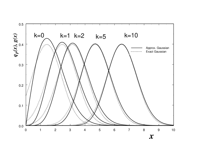
Figure 1:

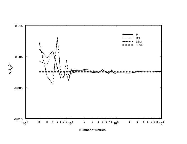
Figure 2:

Figure 3:

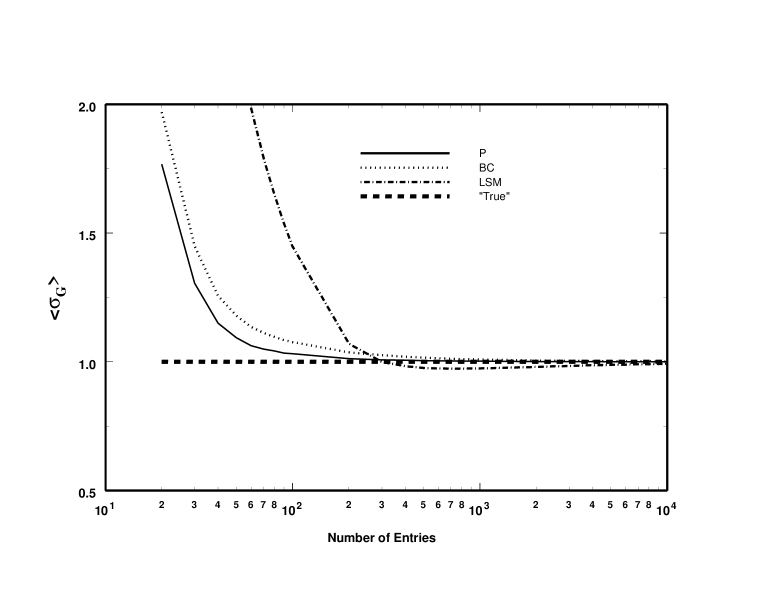
Figure 4:

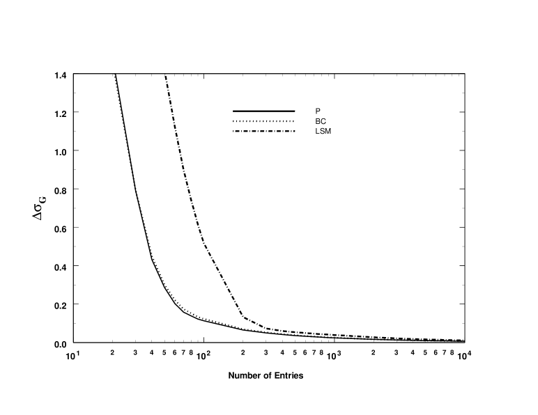
Figure 5:

Figure 6:

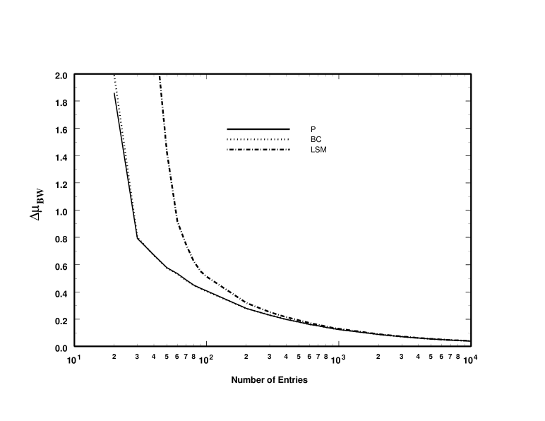
Figure 7:

Figure 8:

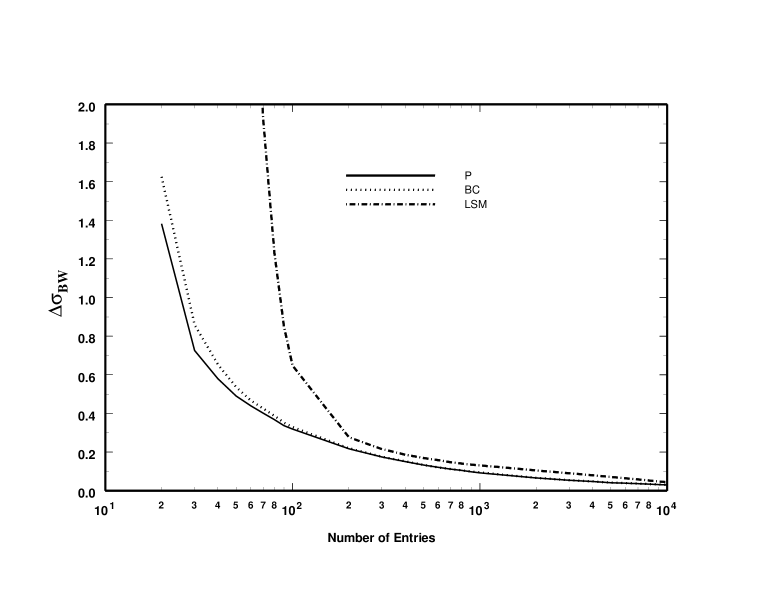
Figure 9:

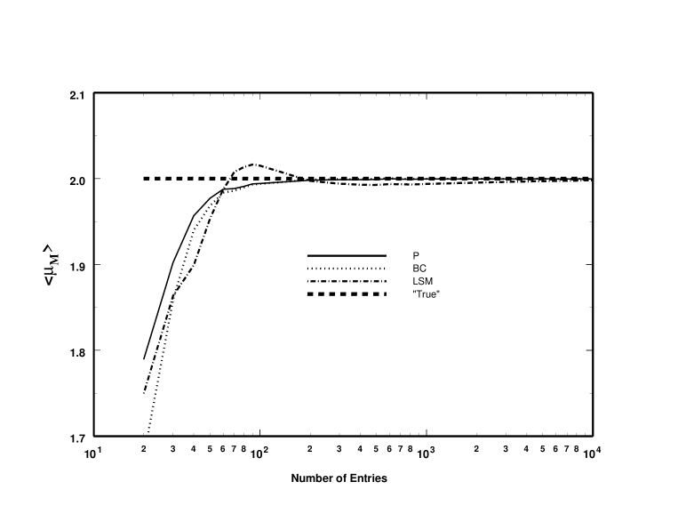
Figure 10:

Figure 11:

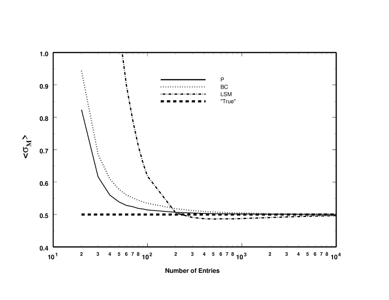
Figure 12:

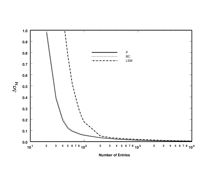
Figure 13:

References

- [1] S. Brandt,”Statistical and Computational Methods in Data Analysis”, North-Holland Publ.Co, Amsterdam, 1970.
- [2] W. T. Eadie, D. Drijard, F. E. James, M. Ross and B. Sadoulet, ”Statistical Methods in Experimental Physics”,North-Holland Publishing Company, 1971.
- [3] S. Baker and R. D. Cousins, Nuclear Instruments and Methods in Physics Research 221 (1984) 437-442.
- [4] G. E. P. Box and G. C. Tiao, ”Bayesian Inference in Statistical Analysis”, John Wiley and Sons, Inc. (Edition Published 1992).
- [5] D. G. Papageorgiou, I. N. Demetropoulos, I. E. Lagaris, Comput. Phys. Commun. 109 (1998) 227-249.