EUROPEAN LABORATORY FOR PARTICLE PHYSICS

CERN-EP/99-154

29 October 1999

Journal Version

22 November 1999

Tau Decays with Neutral Kaons

The OPAL Collaboration

The branching ratio of the $\tau$ lepton to a neutral kaon meson is measured from a sample of approximately 200,000 $\tau$ decays recorded by the OPAL detector at centre-of-mass energies near the $\mathrm{Z}^{0}$ resonance. The measurement is based on two samples which identify one-prong $\tau$ decays with $\mathrm{K^{0}_{L}}$ and $\mathrm{K^{0}_{S}}$ mesons. The combined branching ratios are measured to be

$$B(\tau^{-}\rightarrow\pi^{-}\overline{\mathrm{K}}{}^{0}\nu_{\tau}) = {(9.33\pm 0.68\pm 0.49})\times 10^{-3},$$

$$B(\tau^{-}\rightarrow\pi^{-}\overline{\mathrm{K}}{}^{0}\mbox{\small$[\geq 1\pi^{0}]$}\nu_{\tau}) = {(3.24\pm 0.74\pm 0.66})\times 10^{-3},$$

$$B(\tau^{-}\rightarrow\mathrm{K}^{-}\mathrm{K}{}^{0}{\mbox{\small$[\geq 0\pi^{0}]$}}\nu_{\tau}) = {(3.30\pm 0.55\pm 0.39})\times 10^{-3},$$

where the first error is statistical and the second systematic.

(To be submitted to European Physical Journal C)

The OPAL Collaboration

G. Abbiendi², K. Ackerstaff⁸, P.F. Akesson³, G. Alexander²³, J. Allison¹⁶, K.J. Anderson⁹, S. Arcelli¹⁷, S. Asai²⁴, S.F. Ashby¹, D. Axen²⁹, G. Azuelos^18,a, I. Bailey²⁸, A.H. Ball⁸, E. Barberio⁸, R.J. Barlow¹⁶, J.R. Batley⁵, S. Baumann³, T. Behnke²⁷, K.W. Bell²⁰, G. Bella²³, A. Bellerive⁹, S. Bentvelsen⁸, S. Bethke^14,i, S. Betts¹⁵, O. Biebel^14,i, A. Biguzzi⁵, I.J. Bloodworth¹, P. Bock¹¹, J. Böhme^14,h, O. Boeriu¹⁰, D. Bonacorsi², M. Boutemeur³³, S. Braibant⁸, P. Bright-Thomas¹, L. Brigliadori², R.M. Brown²⁰, H.J. Burckhart⁸, P. Capiluppi², R.K. Carnegie⁶, A.A. Carter¹³, J.R. Carter⁵, C.Y. Chang¹⁷, D.G. Charlton^1,b, D. Chrisman⁴, C. Ciocca², P.E.L. Clarke¹⁵, E. Clay¹⁵, I. Cohen²³, J.E. Conboy¹⁵, O.C. Cooke⁸, J. Couchman¹⁵, C. Couyoumtzelis¹³, R.L. Coxe⁹, M. Cuffiani², S. Dado²², G.M. Dallavalle², S. Dallison¹⁶, R. Davis³⁰, A. de Roeck⁸, P. Dervan¹⁵, K. Desch²⁷, B. Dienes^32,h, M.S. Dixit⁷, M. Donkers⁶, J. Dubbert³³, E. Duchovni²⁶, G. Duckeck³³, I.P. Duerdoth¹⁶, P.G. Estabrooks⁶, E. Etzion²³, F. Fabbri², A. Fanfani², M. Fanti², A.A. Faust³⁰, L. Feld¹⁰, P. Ferrari¹², F. Fiedler²⁷, M. Fierro², I. Fleck¹⁰, A. Frey⁸, A. Fürtjes⁸, D.I. Futyan¹⁶, P. Gagnon¹², J.W. Gary⁴, G. Gaycken²⁷, C. Geich-Gimbel³, G. Giacomelli², P. Giacomelli², D.M. Gingrich^30,a, D. Glenzinski⁹, J. Goldberg²², W. Gorn⁴, C. Grandi², K. Graham²⁸, E. Gross²⁶, J. Grunhaus²³, M. Gruwé²⁷, C. Hajdu³¹ G.G. Hanson¹², M. Hansroul⁸, M. Hapke¹³, K. Harder²⁷, A. Harel²², C.K. Hargrove⁷, M. Harin-Dirac⁴, M. Hauschild⁸, C.M. Hawkes¹, R. Hawkings²⁷, R.J. Hemingway⁶, G. Herten¹⁰, R.D. Heuer²⁷, M.D. Hildreth⁸, J.C. Hill⁵, P.R. Hobson²⁵, A. Hocker⁹, K. Hoffman⁸, R.J. Homer¹, A.K. Honma⁸, D. Horváth^31,c, K.R. Hossain³⁰, R. Howard²⁹, P. Hüntemeyer²⁷, P. Igo-Kemenes¹¹, D.C. Imrie²⁵, K. Ishii²⁴, F.R. Jacob²⁰, A. Jawahery¹⁷, H. Jeremie¹⁸, M. Jimack¹, C.R. Jones⁵, P. Jovanovic¹, T.R. Junk⁶, N. Kanaya²⁴, J. Kanzaki²⁴, G. Karapetian¹⁸, D. Karlen⁶, V. Kartvelishvili¹⁶, K. Kawagoe²⁴, T. Kawamoto²⁴, P.I. Kayal³⁰, R.K. Keeler²⁸, R.G. Kellogg¹⁷, B.W. Kennedy²⁰, D.H. Kim¹⁹, A. Klier²⁶, T. Kobayashi²⁴, M. Kobel³, T.P. Kokott³, M. Kolrep¹⁰, S. Komamiya²⁴, R.V. Kowalewski²⁸, T. Kress⁴, P. Krieger⁶, J. von Krogh¹¹, T. Kuhl³, M. Kupper²⁶, P. Kyberd¹³, G.D. Lafferty¹⁶, H. Landsman²², D. Lanske¹⁴, J. Lauber¹⁵, I. Lawson²⁸, J.G. Layter⁴, D. Lellouch²⁶, J. Letts¹², L. Levinson²⁶, R. Liebisch¹¹, J. Lillich¹⁰, B. List⁸, C. Littlewood⁵, A.W. Lloyd¹, S.L. Lloyd¹³, F.K. Loebinger¹⁶, G.D. Long²⁸, M.J. Losty⁷, J. Lu²⁹, J. Ludwig¹⁰, A. Macchiolo¹⁸, A. Macpherson³⁰, W. Mader³, M. Mannelli⁸, S. Marcellini², T.E. Marchant¹⁶, A.J. Martin¹³, J.P. Martin¹⁸, G. Martinez¹⁷, T. Mashimo²⁴, P. Mättig²⁶, W.J. McDonald³⁰, J. McKenna²⁹, E.A. Mckigney¹⁵, T.J. McMahon¹, R.A. McPherson²⁸, F. Meijers⁸, P. Mendez-Lorenzo³³, F.S. Merritt⁹, H. Mes⁷, I. Meyer⁵, A. Michelini², S. Mihara²⁴, G. Mikenberg²⁶, D.J. Miller¹⁵, W. Mohr¹⁰, A. Montanari², T. Mori²⁴, K. Nagai⁸, I. Nakamura²⁴, H.A. Neal^12,f, R. Nisius⁸, S.W. O’Neale¹, F.G. Oakham⁷, F. Odorici², H.O. Ogren¹², A. Okpara¹¹, M.J. Oreglia⁹, S. Orito²⁴, G. Pásztor³¹, J.R. Pater¹⁶, G.N. Patrick²⁰, J. Patt¹⁰, R. Perez-Ochoa⁸, S. Petzold²⁷, P. Pfeifenschneider¹⁴, J.E. Pilcher⁹, J. Pinfold³⁰, D.E. Plane⁸, B. Poli², J. Polok⁸, M. Przybycień^8,d, A. Quadt⁸, C. Rembser⁸, H. Rick⁸, S.A. Robins²², N. Rodning³⁰, J.M. Roney²⁸, S. Rosati³, K. Roscoe¹⁶, A.M. Rossi², Y. Rozen²², K. Runge¹⁰, O. Runolfsson⁸, D.R. Rust¹², K. Sachs¹⁰, T. Saeki²⁴, O. Sahr³³, W.M. Sang²⁵, E.K.G. Sarkisyan²³, C. Sbarra²⁸, A.D. Schaile³³, O. Schaile³³, P. Scharff-Hansen⁸, J. Schieck¹¹, S. Schmitt¹¹, A. Schöning⁸, M. Schröder⁸, M. Schumacher³, C. Schwick⁸, W.G. Scott²⁰, R. Seuster^14,h, T.G. Shears⁸, B.C. Shen⁴, C.H. Shepherd-Themistocleous⁵, P. Sherwood¹⁵, G.P. Siroli², A. Skuja¹⁷, A.M. Smith⁸, G.A. Snow¹⁷, R. Sobie²⁸, S. Söldner-Rembold^10,e, S. Spagnolo²⁰, M. Sproston²⁰, A. Stahl³, K. Stephens¹⁶, K. Stoll¹⁰, D. Strom¹⁹, R. Ströhmer³³, B. Surrow⁸, S.D. Talbot¹, P. Taras¹⁸, S. Tarem²², R. Teuscher⁹, M. Thiergen¹⁰, J. Thomas¹⁵, M.A. Thomson⁸, E. Torrence⁸, S. Towers⁶, T. Trefzger³³, I. Trigger¹⁸, Z. Trócsányi^32,g, E. Tsur²³, M.F. Turner-Watson¹, I. Ueda²⁴, R. Van Kooten¹², P. Vannerem¹⁰, M. Verzocchi⁸, H. Voss³, F. Wäckerle¹⁰, D. Waller⁶, C.P. Ward⁵, D.R. Ward⁵, P.M. Watkins¹, A.T. Watson¹, N.K. Watson¹, P.S. Wells⁸, T. Wengler⁸, N. Wermes³, D. Wetterling¹¹ J.S. White⁶, G.W. Wilson¹⁶, J.A. Wilson¹, T.R. Wyatt¹⁶, S. Yamashita²⁴, V. Zacek¹⁸, D. Zer-Zion⁸

¹School of Physics and Astronomy, University of Birmingham, Birmingham B15 2TT, UK
²Dipartimento di Fisica dell’ Università di Bologna and INFN, I-40126 Bologna, Italy
³Physikalisches Institut, Universität Bonn, D-53115 Bonn, Germany
⁴Department of Physics, University of California, Riverside CA 92521, USA
⁵Cavendish Laboratory, Cambridge CB3 0HE, UK
⁶Ottawa-Carleton Institute for Physics, Department of Physics, Carleton University, Ottawa, Ontario K1S 5B6, Canada
⁷Centre for Research in Particle Physics, Carleton University, Ottawa, Ontario K1S 5B6, Canada
⁸CERN, European Organisation for Particle Physics, CH-1211 Geneva 23, Switzerland
⁹Enrico Fermi Institute and Department of Physics, University of Chicago, Chicago IL 60637, USA
¹⁰Fakultät für Physik, Albert Ludwigs Universität, D-79104 Freiburg, Germany
¹¹Physikalisches Institut, Universität Heidelberg, D-69120 Heidelberg, Germany
¹²Indiana University, Department of Physics, Swain Hall West 117, Bloomington IN 47405, USA
¹³Queen Mary and Westfield College, University of London, London E1 4NS, UK
¹⁴Technische Hochschule Aachen, III Physikalisches Institut, Sommerfeldstrasse 26-28, D-52056 Aachen, Germany
¹⁵University College London, London WC1E 6BT, UK
¹⁶Department of Physics, Schuster Laboratory, The University, Manchester M13 9PL, UK
¹⁷Department of Physics, University of Maryland, College Park, MD 20742, USA
¹⁸Laboratoire de Physique Nucléaire, Université de Montréal, Montréal, Quebec H3C 3J7, Canada
¹⁹University of Oregon, Department of Physics, Eugene OR 97403, USA
²⁰CLRC Rutherford Appleton Laboratory, Chilton, Didcot, Oxfordshire OX11 0QX, UK
²²Department of Physics, Technion-Israel Institute of Technology, Haifa 32000, Israel
²³Department of Physics and Astronomy, Tel Aviv University, Tel Aviv 69978, Israel
²⁴International Centre for Elementary Particle Physics and Department of Physics, University of Tokyo, Tokyo 113-0033, and Kobe University, Kobe 657-8501, Japan
²⁵Institute of Physical and Environmental Sciences, Brunel University, Uxbridge, Middlesex UB8 3PH, UK
²⁶Particle Physics Department, Weizmann Institute of Science, Rehovot 76100, Israel
²⁷Universität Hamburg/DESY, II Institut für Experimental Physik, Notkestrasse 85, D-22607 Hamburg, Germany
²⁸University of Victoria, Department of Physics, P O Box 3055, Victoria BC V8W 3P6, Canada
²⁹University of British Columbia, Department of Physics, Vancouver BC V6T 1Z1, Canada
³⁰University of Alberta, Department of Physics, Edmonton AB T6G 2J1, Canada
³¹Research Institute for Particle and Nuclear Physics, H-1525 Budapest, P O Box 49, Hungary
³²Institute of Nuclear Research, H-4001 Debrecen, P O Box 51, Hungary
³³Ludwigs-Maximilians-Universität München, Sektion Physik, Am Coulombwall 1, D-85748 Garching, Germany

^a and at TRIUMF, Vancouver, Canada V6T 2A3
^b and Royal Society University Research Fellow
^c and Institute of Nuclear Research, Debrecen, Hungary
^d and University of Mining and Metallurgy, Cracow
^e and Heisenberg Fellow
^f now at Yale University, Dept of Physics, New Haven, USA
^g and Department of Experimental Physics, Lajos Kossuth University, Debrecen, Hungary
^h and MPI München
ⁱ now at MPI für Physik, 80805 München.

1 Introduction

The large samples of $\mathrm{Z^{0}}$ events collected at $\mathrm{e^{+}}\mathrm{e^{-}}$ colliders over the past ten years have made it possible to study resonance dynamics and test low energy QCD using the decays of $\tau$ leptons to kaons. In this paper, measurements of the branching ratios of the $\tau^{-}\rightarrow\pi^{-}\overline{\mathrm{K}}{}^{0}\nu_{\tau}$, $\tau^{-}\rightarrow\pi^{-}\overline{\mathrm{K}}{}^{0}\mbox{\small$[\geq 1\pi^{0}]$}\nu_{\tau}$ and $\tau^{-}\rightarrow\mathrm{K}^{-}\mathrm{K}{}^{0}{\mbox{\small$[\geq 0\pi^{0}]$}}\nu_{\tau}$ decay modes are presented. These measurements are based on two samples that identify $\tau$ decays with $\mathrm{K^{0}_{L}}$ and $\mathrm{K^{0}_{S}}$ mesons. The $\mathrm{K^{0}_{L}}$ mesons are identified by their one-prong nature accompanied by a large deposition of energy in the hadron calorimeter while the $\mathrm{K^{0}_{S}}$ mesons are identified through their decay into two charged pions. The selected number of $\tau^{-}\rightarrow\pi^{-}\overline{\mathrm{K}}{}^{0}\mathrm{K}{}^{0}\nu_{\tau}$ decays is very small and is treated as background in this analysis.

The results presented here are extracted from the data collected between 1991 and 1995 at energies close to the $\mathrm{Z^{0}}$ resonance, corresponding to an integrated luminosity of 163 pb^-1, with the OPAL detector at LEP. A description of the OPAL detector can be found in [1]. The performance and particle identification capabilities of the OPAL jet chamber are described in [2]. The $\tau$ pair Monte Carlo samples used in this analysis are generated using the KORALZ 4.0 package [3]. The dynamics of the $\tau$ decays are simulated with the Tauola 2.4 decay library [4]. The Monte Carlo events are then passed through the OPAL detector simulation [5].

2 Selection of $\tau^{+}\tau^{-}$ events

The procedure used to select $\mathrm{Z^{0}}\rightarrow\tau^{+}\tau^{-}$ events is identical to that described in previous OPAL publications [6, 7]. The decay of the $\mathrm{Z}^{0}$ produces two back-to-back taus. The taus are highly relativistic so that the decay products are strongly collimated. As a result it is convenient to treat each $\tau$ decay as a jet, where charged tracks and clusters are assigned to cones of half-angle $35^{\circ}$ [6, 7]. In order to avoid regions of non-uniform calorimeter response, the two $\tau$ jets are restricted to the barrel region of the OPAL detector by requiring that the average polar angle of the two jets satisfies $\overline{|cos\theta|}<0.68$. The level of contamination from multihadronic events ($\mathrm{e^{+}}\mathrm{e^{-}}\!\!\rightarrow\!\mathrm{q}\bar{\mathrm{q}}$) is significantly reduced by requiring not more than six tracks and ten electromagnetic clusters per event. Bhabha $(\mathrm{e^{+}}\mathrm{e^{-}}\!\!\rightarrow\!\mathrm{e^{+}}\mathrm{e^{-}})$ and muon pair $(\mathrm{e^{+}}\mathrm{e^{-}}\!\!\rightarrow\!\mathrm{\mu^{+}}\mathrm{\mu^{-}})$ events are removed by rejecting events where the total electromagnetic energy and the scalar sum of the track momenta are close to the centre-of-mass energy. Two-photon events, $\mathrm{e^{+}}\mathrm{e^{-}}\!\!\rightarrow\!(\mathrm{e^{+}}\mathrm{e^{-}})\mathrm{e^{+}}\mathrm{e^{-}}$ or $\mathrm{e^{+}}\mathrm{e^{-}}\!\!\rightarrow\!(\mathrm{e^{+}}\mathrm{e^{-}})\mathrm{\mu^{+}}\mathrm{\mu^{-}}$, are removed by rejecting events which have little visible energy in the electromagnetic calorimeter and a large acollinearity angle between the two jets.

A total of $100925$ events are selected for the $\mathrm{K}{}^{0}_{\mathrm{L}}$ sample and $85789$ events are selected for the $\mathrm{K}{}^{0}_{\mathrm{S}}$ sample from the 1991-1995 data set. The different number of $\tau^{+}\tau^{-}$ events in the two samples is due to different detector status requirements used in each selection. The fraction of background from non-$\tau$ sources is $(1.6\pm 0.1)$% [6, 7].

3 Selection of $\tau^{-}\rightarrow\mathrm{X}^{-}\;\overline{\mathrm{K}}{}^{0}_{\mathrm{L}}\nu_{\tau}$ decays

The selection of $\tau$ decays into to a final state containing at least one $\mathrm{K^{0}_{L}}$ meson follows a simple cut-based procedure. Some $\mathrm{K^{0}_{S}}$ mesons will be selected in this $\mathrm{K^{0}_{L}}$ selection. In particular, $\mathrm{K^{0}_{S}}$ mesons that decay late in the jet chamber, the solenoid or the electromagnetic calorimeter, will be indistinguishable from $\mathrm{K^{0}_{L}}$ mesons and are considered to be part of the $\mathrm{K^{0}_{L}}$ signal. The Monte Carlo simulation predicts that the $\mathrm{K^{0}}$ component identified by the $\mathrm{K^{0}_{L}}$ selection is composed of 86% $\mathrm{K^{0}_{L}}$ and 14% $\mathrm{K^{0}_{S}}$ mesons.

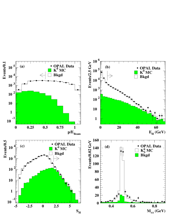
Figure 1: The first three plots show the $\mathrm{K^{0}_{L}}$ selection variables: (a) the momentum divided by the beam energy $(p/\mbox{$E_{\mathrm{beam}}$})$, (b) the hadronic calorimeter energy ($E_{\mathrm{HB}}$) and (c) $S_{\mathrm{H}}=(E_{\mathrm{H}}-p)/\sigma_{\mathrm{H}}$. The fourth plot shows the mass distribution of jets which pass the $\mathrm{K^{0}_{S}}$ selection. In each case, jets which pass all of the selection requirements except for the variable in question are plotted.

First, each jet must contain exactly one track pointing to the primary vertex and its momentum divided by the beam energy ($p/\mbox{$E_{\mathrm{beam}}$}$) must be less than 0.5, see fig. 1(a). This requirement removes high-momentum pion decays from the one-prong sample. In order to exclude leptonic background, there must be at least one cluster in the hadron calorimeter and the total amount of energy measured by the hadronic calorimeter within the jet must be greater than 7.5 GeV, see fig. 1(b).

The $\tau^{-}\rightarrow\mathrm{X}^{-}\;\overline{\mathrm{K}}{}^{0}_{\mathrm{L}}\nu_{\tau}$ decays will deposit on average more energy in the hadron calorimeter than most other $\tau$ decays. This property is exploited using the variable, $S_{\mathrm{H}}=(E_{\mathrm{H}}-p)/\sigma_{\mathrm{H}}$, where $E_{\mathrm{H}}$ is the total energy deposited in the hadron calorimeter for the jet, $p$ is the momentum of the track and $\sigma_{\mathrm{H}}/E_{\mathrm{H}}=0.165+0.847/\sqrt{E_{\mathrm{H}}}$ is the hadron calorimeter resolution. The energy is calibrated and the resolution is measured using pions from $\tau$ decays that do not interact in the electromagnetic calorimeter. Events with $S_{\mathrm{H}}\geq 2.0$ are classified as $\mathrm{X}^{-}\;\overline{\mathrm{K}}{}^{0}_{\mathrm{L}}$ decays, see fig. 1(c). A total of $305$ candidates are selected using the above requirements. The background is estimated to be 24% from other $\tau$ decays and 6% from $\mathrm{e^{+}}\mathrm{e^{-}}\!\!\rightarrow\!\mathrm{q}\bar{\mathrm{q}}$ events. The primary $\tau$ background consists of $\tau^{-}\rightarrow\pi^{-}\nu_{\tau}$, $\tau^{-}\rightarrow\rho(770)^{-}\nu_{\tau}$ and $\tau^{-}\rightarrow\mbox{a}_{1}(1260)^{-}\nu_{\tau}$ decays.

The sample of $\tau^{-}\rightarrow\mathrm{X}^{-}\;\overline{\mathrm{K}}{}^{0}_{\mathrm{L}}\nu_{\tau}$ decays is subdivided into two sets: one in which the track is identified as a pion and another in which the track is identified as a kaon. The sample with charged pions is then passed through an additional selection which identifies those decays that include a $\pi^{0}$ meson. The identification of the charged hadron uses the normalized specific energy loss defined as $(({\mathrm{d}}E/{\mathrm{d}}x)_{\mathrm{measured}}-({\mathrm{d}}E/{\mathrm{d}}x)_{\mathrm{expected}})/\sigma_{{\mathrm{d}}E/{\mathrm{d}}x}$, where $\sigma_{{\mathrm{d}}E/{\mathrm{d}}x}$ is the ${\mathrm{d}}E/{\mathrm{d}}x$ resolution. Using this quantity, it is possible to separate charged pions and kaons at a level of $2\sigma$ in the momentum range of 2-30 GeV. The expected ${\mathrm{d}}E/{\mathrm{d}}x$ is calculated using the Bethe-Bloch equation parameterised for the OPAL jet chamber [2]. The parameterisation is checked using one-prong hadronic $\tau$ decays by comparing the mean values and widths of the normalised ${\mathrm{d}}E/{\mathrm{d}}x$ distributions in bins of $\beta=p/E$, with $E^{2}=p^{2}+m_{\pi}^{2}$. It is found that a small $\beta$-dependent correction is to be applied to the Monte Carlo. The correction shifts the mean value of the expected ${\mathrm{d}}E/{\mathrm{d}}x$ by up to 10% and the widths by approximately 5%. Charged pions and kaons are separated using a ${\mathrm{d}}E/{\mathrm{d}}x$ probability variable $W$, which is calculated from the normalized ${\mathrm{d}}E/{\mathrm{d}}x$ for each particle species. These are combined into pion and kaon probabilities,

$$\mathrm{P}_{\pi} = W_{\pi}/(W_{\pi}+W_{\mathrm{K}})$$

$$\mathrm{P}_{\mathrm{K}} = W_{\mathrm{K}}/(W_{\pi}+W_{\mathrm{K}}).$$

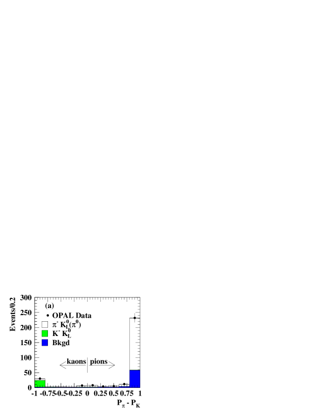
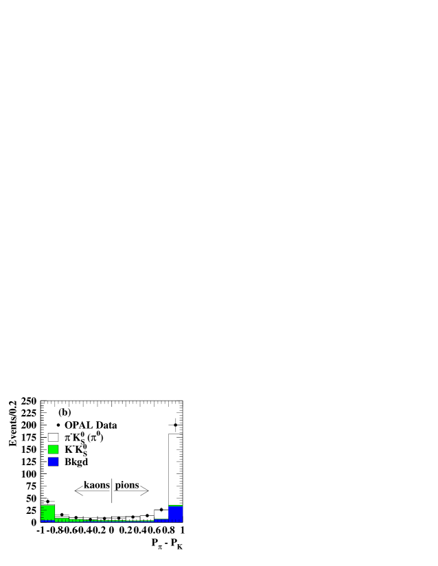
Figure 2: The $\pi/\mathrm{K}$ separation variables. (a) shows the difference of the pion ($P_{\pi}$) and kaon ($P_{\mathrm{K}}$) probabilities, $P_{\pi}-P_{\mathrm{K}}$, for the $\mathrm{K^{0}_{L}}$ sample, (b) shows $P_{\pi}-P_{\mathrm{K}}$ for the $\mathrm{K^{0}_{S}}$ sample.

The distributions of the difference $\mathrm{P}_{\pi}-\mathrm{P}_{\mathrm{K}}$ is shown in fig. 2(a). A track is considered to be a pion if $\mathrm{P}_{\pi}>\mathrm{P}_{\mathrm{K}}$.

A neural network algorithm is used to identify the $\tau^{-}\rightarrow\pi^{-}\overline{\mathrm{K}}{}^{0}\nu_{\tau}$ and $\tau^{-}\rightarrow\pi^{-}\overline{\mathrm{K}}{}^{0}\mbox{\small$[\geq 1\pi^{0}]$}\nu_{\tau}$ decay modes. The neural network algorithm uses 7 variables to identify the $\tau$ jets:

• The total energy of the jet in the electromagnetic calorimeter divided by the beam energy, $E/\mbox{$E_{\mathrm{beam}}$}$.

• The total energy of the jet in the electromagnetic calorimeter divided by the momentum of the track, $E/p$.

• The number of electromagnetic clusters in the jet with an energy greater than 1 GeV.

• The minimum fraction of active lead glass blocks which together contains more than 90% of the total electromagnetic energy of the jet, $F_{90}$.

• The difference in the azimuthal angle between the track and the presampler signal farthest away from the track but still within the jet, $\phi_{\mathrm{PS}}$.

• The difference in theta ($\Delta\theta$) and phi ($\Delta\phi$) between the track and the vector obtained by adding together all the electromagnetic calorimeter clusters in the jet.

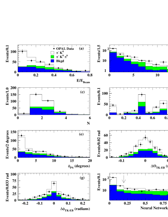
Figure 3: The variables used in the neural network routine for identifying $\pi^{0}$ mesons in the $\mathrm{K^{0}_{L}}$ sample: (a) the electromagnetic energy divided by the beam energy; (b) the ratio of the electromagnetic energy ($E$) with the momentum of the track ($p$); (c) the number of electromagnetic calorimeter clusters ($N$); (d) the fraction of lead glass blocks in the electromagnetic calorimeter with over 90% of the energy in the jet; (e) angle between the position of the track at the presampler and the presampler cluster furthest away from the jet axis; (f) and (g) the difference in theta ($\Delta\theta$) and phi ($\Delta\phi$) between the track and the vector obtained by adding all the clusters in the electromagnetic calorimeter; (h) the output of the neural network, the arrow indicates the cut used to select decays containing $\pi^{0}$ mesons.

The variables used in the neural network and the output are shown in fig. 3. If the neural network output is larger than 0.2 then the decay is considered to contain a $\pi^{0}$ meson.

4 Selection of $\tau^{-}\rightarrow\mathrm{X}^{-}\;\overline{\mathrm{K}}{}^{0}_{\mathrm{S}}\nu_{\tau}$ decays

The algorithm for identifying $\mathrm{K}{}^{0}_{\mathrm{S}}$ candidates is similar to those used in other OPAL analyses (for example, see [9]). The algorithm begins by pairing tracks with opposite charge. Each track must have a minimum transverse momentum of 150 MeV and more than 40 out of a possible 159 hits in the jet chamber. Intersection points of track pairs in the plane perpendicular to the beam axis are considered to be secondary vertex candidates. Each secondary vertex is then required to satisfy the following criteria:

• The radial distance $R_{V}$ from the secondary vertex to the primary vertex must be greater than 10 cm and less than 150 cm.

• The reconstructed momentum vector of the $\mathrm{K}{}^{0}_{\mathrm{S}}$ candidate in the plane perpendicular to the beam axis must point to the beam axis within 1^∘.

• If $R_{V}$ is between 30 and 150 cm (i.e. the secondary vertex is inside the jet chamber volume), then the radius of the first jet chamber hit associated with either of the two tracks ($R_{1}$) must satisfy $R_{V}-R_{1}<5$ cm.

• If $R_{V}$ is between 10 and 30 cm (not inside the jet chamber volume), then the impact parameter of the track is required to exceed 1 mm.

• The invariant mass of the pair of tracks, assuming both tracks to be electrons from a photon conversion, is required to be greater than 100 MeV.

The $\tau$ jet is required to have at least one $\mathrm{K^{0}_{S}}$ candidate. If there is more than one candidate then only the secondary vertex with an invariant mass closest to the true $\mathrm{K^{0}_{S}}$ mass is retained. In addition, each jet is required to have only one additional track, called the primary track.

A number of additional criteria are applied to reduce the background from other $\tau$ decays. Each track associated with the $\mathrm{K^{0}_{S}}$ must have $p>1$ GeV and must not have any hits in the axial regions of the vertex drift chamber, which extends radially from 10.3 to 16.2 cm. If the radial distance to the secondary vertex is between 30 and 150 cm, tracks with hits in the stereo region of the vertex drift chamber, which extends radially from 18.8 to 21.3 cm, are rejected.

Candidate decays containing photon conversions identified with an algorithm described in [10], are rejected. Finally, the mass of the jet (assuming that the primary track is a pion) must be less than 2 GeV and the invariant mass of the $\mathrm{K}{}^{0}_{\mathrm{S}}$ candidate is required to be between 0.4 and 0.6 GeV, see fig. 1(d). A total of $349$ candidates are obtained with a background of approximately 10%, consisting primarily of $\tau^{-}\rightarrow\rho(770)^{-}\nu_{\tau}$ and $\tau^{-}\rightarrow\mbox{a}_{1}(1260)^{-}\nu_{\tau}$ decays.

The sample of $\tau^{-}\rightarrow\mathrm{X}^{-}\;\overline{\mathrm{K}}{}^{0}_{\mathrm{S}}\nu_{\tau}$ decays is subdivided into two sets: one in which the primary track is identified as a pion and another in which the primary track is identified as a kaon, as described in section 3. In fig. 2(b), the difference of the pion ($\mathrm{P}_{\pi}$) and kaon ($\mathrm{P}_{\mathrm{K}}$) probability weight ratios is shown for tracks identified as charged pions and kaons. A decay is considered to contain a $\pi^{-}$ if $\mathrm{P}_{\pi}>\mathrm{P}_{\mathrm{K}}$.

A neural network algorithm is used to identify the $\tau^{-}\rightarrow\pi^{-}\overline{\mathrm{K}}{}^{0}\nu_{\tau}$ and $\tau^{-}\rightarrow\pi^{-}\overline{\mathrm{K}}{}^{0}\mbox{\small$[\geq 1\pi^{0}]$}\nu_{\tau}$ decay modes. The neural network algorithm is similar to the one used in the $\mathrm{K^{0}_{L}}$ analysis; the differences are due to the different topologies of the two selections. The neural network algorithm for this selection uses 6 variables to identify the $\tau$ jets:

• The total energy of the jet in the electromagnetic calorimeter divided by the scalar sum of the momenta of the tracks, $E/p$.

• The number of clusters in the electromagnetic calorimeter with energy greater than 1 GeV in the jet.

• The minimum fraction of active lead glass blocks which together contains more than 90% of the total electromagnetic energy of the jet, $F_{90}$.

• The total presampler multiplicity in the jet.

• The difference in theta ($\Delta\theta$) and phi ($\Delta\phi$) between the vector obtained by adding together all the tracks and the vector obtained by adding together all the clusters in the electromagnetic calorimeter associated to the jet.

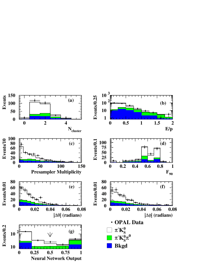
Figure 4: The variables used in the neural network routine for identifying $\pi^{0}$ mesons in the $\mathrm{K^{0}_{S}}$ sample: (a) the number of clusters in the electromagnetic calorimeter; (b) the ratio of the total energy in the electromagnetic calorimeter divided by the total scalar momentum of the tracks; (c) the presampler multiplicity, (d) the fraction of lead glass blocks in the electromagnetic calorimeter with over 90% of the energy in the jet; (e) and (f) the difference in theta ($\Delta\theta$) and phi ($\Delta\phi$) between the vector obtained by adding all the tracks and the vector obtained by adding all the clusters in the electromagnetic calorimeter; (g) the output of the neural network, the arrow indicates the cut used to select decays containing $\pi^{0}$ mesons.

The variables used in the neural network algorithm are shown in figs. 4(a-f). A decay is considered to contain a $\pi^{0}$ if the neural network output, shown in fig. 4(g), is greater than 0.5.

5 Branching ratios

The branching ratios of the $\tau^{-}\rightarrow\pi^{-}\overline{\mathrm{K}}{}^{0}\nu_{\tau}$, $\tau^{-}\rightarrow\pi^{-}\overline{\mathrm{K}}{}^{0}\mbox{\small$[\geq 1\pi^{0}]$}\nu_{\tau}$ and $\tau^{-}\rightarrow\mathrm{K}^{-}\mathrm{K}{}^{0}{\mbox{\small$[\geq 0\pi^{0}]$}}\nu_{\tau}$ decay modes are calculated independently for the $\tau$ jets containing $\mathrm{K^{0}_{L}}$ and $\mathrm{K^{0}_{S}}$ decays. However, for a given data sample, the three branching ratios are calculated simultaneously. Each selection can be characterised in terms of the efficiency for detecting each decay mode $i$, the branching ratio of each mode and the number of events selected in the data:

$$\epsilon_{i1}B_{1}+\epsilon_{i2}B_{2}+\epsilon_{i3}B_{3}+\sum_{k=4}^{M}\epsilon_{ik}B_{k}=\frac{N_{i}-N_{i}^{{\mbox{\scriptsize non}}-\tau}}{N_{\tau}(1-f^{{\mbox{\scriptsize non}}-\tau})}$$

where $N_{i}$ is the number of data events that pass the selection $i$, $\epsilon_{ij}$ ($j=1,3$) are the efficiencies for selecting signal $j$ using selection $i$, $\epsilon_{ik}$ ($k=4,\ldots,M$) are the efficiencies for selecting the $\tau$ background modes using selection $i$ and $M$ is the number of the $\tau$ decay modes. The branching ratios of the signal channels and backgrounds are $B_{j}$ ($j=1,3$) and $B_{k}$ ($k=4,\dots,M$), respectively. The fraction of non-$\tau$ events in the $\tau$ pair sample is $f^{{\mbox{\scriptsize non}}-\tau}$, $N_{\tau}$ is the total number of taus in the data that pass the $\tau$ pair selection and $N_{i}^{{\mbox{\scriptsize non}}-\tau}$ is the non-$\tau$ background present in each selection $i$. The selection efficiencies ($\epsilon_{ij}$) for both signal and background are determined from Monte Carlo simulation. The $\tau$ background branching ratios are taken from the Particle Data Group compilation [11].

Solving the three simultaneous equations yields the branching ratios in each sample of selected events. A small correction is applied to the branching ratios to account for any biases introduced into the $\tau$ pair sample by the $\tau$ pair selection. The bias factor is defined as the ratio of the fraction of the selected decays in a sample of $\tau$ decays after the $\tau$ selection is applied to the fraction before the selection. The bias factors are calculated using approximately 2.2 million simulated $\tau^{+}\tau^{-}$ events. The bias factors for the $\tau^{-}\rightarrow\pi^{-}\overline{\mathrm{K}}{}^{0}\nu_{\tau}$, $\tau^{-}\rightarrow\pi^{-}\overline{\mathrm{K}}{}^{0}\mbox{\small$[\geq 1\pi^{0}]$}\nu_{\tau}$ and $\tau^{-}\rightarrow\mathrm{K}^{-}\mathrm{K}{}^{0}{\mbox{\small$[\geq 0\pi^{0}]$}}\nu_{\tau}$ decays are found to be $0.99\pm 0.01$, $1.00\pm 0.01$ and $1.00\pm 0.01$ for the branching ratios obtained from the $\mathrm{K}{}^{0}_{\mathrm{L}}$ sample, and $0.99\pm 0.01$, $1.01\pm 0.03$ and $0.99\pm 0.02$ for the branching ratios obtained from the $\mathrm{K}{}^{0}_{\mathrm{S}}$ sample. The uncertainties on the measurements are statistical only.

The $\mathrm{K^{0}_{L}}$ ($\mathrm{K^{0}_{S}}$) selection identifies $178$ ($199$) $\tau^{-}\rightarrow\pi^{-}\overline{\mathrm{K}}{}^{0}\nu_{\tau}$ decays, $81$ ($67$) $\tau^{-}\rightarrow\pi^{-}\overline{\mathrm{K}}{}^{0}\mbox{\small$[\geq 1\pi^{0}]$}\nu_{\tau}$ decays and $41$ ($83$) $\tau^{-}\rightarrow\mathrm{K}^{-}\mathrm{K}{}^{0}{\mbox{\small$[\geq 0\pi^{0}]$}}\nu_{\tau}$ decays. The efficiency matrix for each sample is given in table 1.

The branching ratios obtained from the $\mathrm{K}{}^{0}_{\mathrm{L}}$ sample are

$$B(\tau^{-}\rightarrow\pi^{-}\overline{\mathrm{K}}{}^{0}\nu_{\tau}) = (9.1\pm 0.9\pm 0.6)\times 10^{-3},$$

$$B(\tau^{-}\rightarrow\pi^{-}\overline{\mathrm{K}}{}^{0}\mbox{\small$[\geq 1\pi^{0}]$}\nu_{\tau}) = (3.6\pm 1.3\pm 1.0)\times 10^{-3},$$

$$B(\tau^{-}\rightarrow\mathrm{K}^{-}\mathrm{K}{}^{0}{\mbox{\small$[\geq 0\pi^{0}]$}}\nu_{\tau}) = (3.3\pm 0.9\pm 0.7)\times 10^{-3},$$

while the branching ratios obtained from the $\mathrm{K}{}^{0}_{\mathrm{S}}$ sample are

$$B(\tau^{-}\rightarrow\pi^{-}\overline{\mathrm{K}}{}^{0}\nu_{\tau}) = (9.6\pm 1.0\pm 0.7)\times 10^{-3},$$

$$B(\tau^{-}\rightarrow\pi^{-}\overline{\mathrm{K}}{}^{0}\mbox{\small$[\geq 1\pi^{0}]$}\nu_{\tau}) = (3.0\pm 0.9\pm 0.9)\times 10^{-3},$$

$$B(\tau^{-}\rightarrow\mathrm{K}^{-}\mathrm{K}{}^{0}{\mbox{\small$[\geq 0\pi^{0}]$}}\nu_{\tau}) = (3.3\pm 0.7\pm 0.5)\times 10^{-3},$$

where the first error is statistical and the second is systematic.

6 Systematic errors

The systematic uncertainties on the branching ratios are presented in table 2. The dominant contributions to the systematic uncertainty arises from the efficiency of the two selections, the uncertainty of the backgrounds, the modelling of the ${\mathrm{d}}E/{\mathrm{d}}x$, the identification of the $\pi^{0}$ and the modelling of Monte Carlo. These uncertainties are discussed in more detail below. In addition, there are straightforward contributions from the limited statistics of the Monte Carlo samples used to estimate the selection efficiencies and from the uncertainties on the bias factors. The systematic error on the branching ratios due to the Monte Carlo statistics is calculated directly from the statistical uncertainties on the elements of the inverse efficiency matrix [12]. The systematic error on each branching ratio due to the bias factor is calculated directly from the bias factor error.

$\mathrm{K^{0}_{L}}$ and $\mathrm{K^{0}_{S}}$ selection efficiencies:

The $\mathrm{K^{0}_{L}}$ selection efficiency is sensitive to the calibration of the momentum, the energy measured by the hadron calorimeter and the resolution of the hadron calorimeter. The uncertainty on the momentum scale is typically better than 1% [7]. The uncertainty in the energy scale of the hadron calorimeter is obtained by studying a sample of single charged hadrons from $\tau$ decays, the level of agreement between the data and Monte Carlo is 1.5%. The uncertainty due to the measurement of the resolution of the hadron calorimeter is estimated by varying the resolution within its uncertainties. Also, the shower containment is examined by looking at the leakage of energy out of the back of the hadron calorimeter. It is found that about 8% of $\mathrm{K^{0}_{L}}$ decays may not be fully contained, these decays are well modelled by the Monte Carlo and does not result in a systematic uncertainty.

The $\mathrm{K^{0}_{S}}$ selection efficiency is sensitive to the requirements on the impact parameter, the momentum and the number of hits in the stereo and axial regions of the vertex chamber on the tracks associated to the $\mathrm{K^{0}_{S}}$ . The systematic error on the $\mathrm{K^{0}_{S}}$ selection efficiency is determined by dropping each relevant criterion except for the impact parameter resolution. The impact parameter resolution has been shown to have an uncertainty that is typically better than $\pm 20\%$ [8]. Variations of the impact parameter resolution are found to have almost no contribution to the systematic error on the $\mathrm{K^{0}_{S}}$ selection efficiency.

Background estimation:

The systematic error due to the background in the $\mathrm{K^{0}_{L}}$ sample includes the uncertainty in the branching ratios of the background decays, including the $\tau^{-}\rightarrow\pi^{-}\overline{\mathrm{K}}{}^{0}\mathrm{K}{}^{0}\nu_{\tau}$ and $\tau^{-}\rightarrow\pi^{-}\overline{\mathrm{K}}{}^{0}\mathrm{K}{}^{0}\pi^{0}\nu_{\tau}$ decays, as well as the uncertainty from the Monte Carlo statistics [11, 13]. The non-$\mathrm{K^{0}}$ background consists primarily of $\pi^{-}$, $\rho(770)^{-}$ and $\mathrm{a}_{1}(1260)^{-}$ decays in which the decays have a low momentum track with at least one of the final $\pi$ mesons leaving some energy in the hadron calorimeter. To investigate this background, the $\mathrm{K^{0}_{L}}$ selection cut $S_{H}$ is reversed and the invariant mass spectra are studied for each decay mode. The ratios of the data to the Monte Carlo simulation are consistent with unity: $0.97\pm 0.02$, $1.04\pm 0.02$ and $0.94\pm 0.06$ for the $\pi^{-}\overline{\mathrm{K}}{}^{0}$, $\pi^{-}\overline{\mathrm{K}}{}^{0}\geq 1\pi^{0}$ and $\mathrm{K^{-}}\mathrm{K^{0}}\geq 0\pi^{0}$ selections, respectively. The various contributions to the systematic error from the background are added in quadrature.

The background in the $\mathrm{K^{0}_{S}}$ sample includes $\tau^{-}\rightarrow\pi^{-}\overline{\mathrm{K}}{}^{0}\mathrm{K}{}^{0}\nu_{\tau}$ and $\tau^{-}\rightarrow\pi^{-}\overline{\mathrm{K}}{}^{0}\mathrm{K}{}^{0}\pi^{0}\nu_{\tau}$ decays, which contain $\mathrm{K^{0}_{S}}$ mesons, and other $\tau$ decays, the uncertainty is composed of the Monte Carlo statistical uncertainty plus a component due to the uncertainty in the branching ratios of these decays [11, 13]. A study of the sidebands of the $m_{\pi\pi}$ distribution (see fig. 1(d)) showed that the background prediction from other $\tau$ decays is observed to be about 20% smaller in the Monte Carlo simulation than in the data. As a result, the background is scaled upward by a factor of 1.2 and a 20% uncertainty is assigned to the background estimate. The background estimate is cross-checked using the invariant mass distributions of the tracks associated with the $\mathrm{K^{0}_{S}}$ candidate for each of the exclusive channels. The ratios of the data to the Monte Carlo simulation are consistent: $1.07\pm 0.12$, $1.09\pm 0.06$ and $0.93\pm 0.11$ for the $\pi^{-}\overline{\mathrm{K}}{}^{0}_{\mathrm{S}}$, $\pi^{-}\overline{\mathrm{K}}{}^{0}_{\mathrm{S}}\geq 1\pi^{0}$ and $\mathrm{K^{-}}\mathrm{K^{0}_{S}}\geq 0\pi^{0}$ selections, respectively. The various contributions to the systematic error from the background are added in quadrature.

Modelling of ${\mathrm{d}}E/{\mathrm{d}}x$:

For both samples, the normalized ${\mathrm{d}}E/{\mathrm{d}}x$ distributions are studied using the sample of single charged hadrons from $\tau$ decays. The uncertainty in the branching ratios is estimated by varying the means of the normalised ${\mathrm{d}}E/{\mathrm{d}}x$ distributions by $\pm 1$ standard deviation of their central values. In addition, to account for possible differences in the ${\mathrm{d}}E/{\mathrm{d}}x$ resolution, the widths of the normalized ${\mathrm{d}}E/{\mathrm{d}}x$ distributions are varied by $\pm 30$%. Due to the three tracks present in the $\mathrm{K^{0}_{S}}$ sample, an additional contribution to the systematic error is obtained by measuring the difference in the branching ratios when two different corrections are applied to the Monte Carlo. The first correction is estimated from the one-prong hadronic tau decays while the second correction is estimated using the sample of pions from the decay of the $\mathrm{K^{0}_{S}}$. The various contributions to the systematic error from the ${\mathrm{d}}E/{\mathrm{d}}x$ modelling are added in quadrature.

Identification of $\pi^{0}$:

Both the $\mathrm{K^{0}_{L}}$ and $\mathrm{K^{0}_{S}}$ samples use a neural network algorithm to separate the $\tau^{-}\rightarrow\pi^{-}\overline{\mathrm{K}}{}^{0}\nu_{\tau}$ and $\tau^{-}\rightarrow\pi^{-}\overline{\mathrm{K}}{}^{0}\mbox{\small$[\geq 1\pi^{0}]$}\nu_{\tau}$ decay modes. The most powerful variable for distinguishing between these two decays is the energy deposited in the electromagnetic calorimeter. The systematic error in the branching ratio is evaluated by shifting the electromagnetic energy scale by $\pm 1\%$; this variation is assigned after studying the differences between data and Monte Carlo in $E/p$ distributions for 3-prong $\tau$ decays.

The uncertainty affecting the $\pi^{0}$ identification also includes the maximum uncertainty when each variable (except in those which include the electromagnetic energy) is individually dropped from the neural network algorithm. These uncertainties are added in quadrature with those obtained from the energy scale uncertainty. The stability of the neural network algorithm is studied by removing all but the two most significant variables from the neural network, the results are within the systematic uncertainties for both samples. As a cross check, the cut on the neural network output for both the $\mathrm{K^{0}_{L}}$ and $\mathrm{K^{0}_{S}}$ samples is varied between 0.1 and 0.8, with the result being consistent within the total systematic uncertainties.

Monte Carlo modelling:

The models used in the Monte Carlo generator can effect both the pion and kaon momentum spectra. This effect can produce biases when determining the $\mathrm{K^{0}}$ identification efficiency, the $\mathrm{K}/\pi$ separation and the $\pi^{0}$ identification. The dynamics of the $\pi^{-}\overline{\mathrm{K}}{}^{0}$ decay mode are well understood. The $\pi^{-}\overline{\mathrm{K}}{}^{0}$ decay mode is generated by Tauola via the $\mathrm{K}^{*}(892)^{-}$ resonance. The $\mathrm{K^{-}}\mathrm{K^{0}}$ final state is generated by Tauola using phase space only.

The $\tau^{-}\rightarrow\pi^{-}\overline{\mathrm{K}}{}^{0}\mbox{\small$[\geq 1\pi^{0}]$}\nu_{\tau}$ decay mode is composed of $\tau^{-}\!\rightarrow\pi^{-}\overline{\mathrm{K}}{}^{0}\pi^{0}\nu_{\tau}$ and $\tau^{-}\!\rightarrow\!\pi^{-}\overline{\mathrm{K}}{}^{0}\pi^{0}\pi^{0}\nu_{\tau}$ decays. The $\tau^{-}\rightarrow\pi^{-}\overline{\mathrm{K}}{}^{0}\pi^{0}\nu_{\tau}$ channel is modelled by Tauola assuming that the decay proceeds via the $\mathrm{K}_{1}(1400)$ resonance. Recent results from ALEPH [14] on one-prong $\tau$ decays with kaons, and OPAL [15] using $\tau^{-}\rightarrow\mathrm{K^{-}}\pi^{-}\pi^{+}\nu_{\tau}$ decays, suggest that the $\tau^{-}\rightarrow\pi^{-}\overline{\mathrm{K}}{}^{0}\pi^{0}\nu_{\tau}$ decay will also proceed via the $\mathrm{K}_{1}(1270)$ resonance. A special Monte Carlo simulation is generated in which the final state is created using the $\mathrm{K}_{1}(1270)$ and $\mathrm{K}_{1}(1400)$ resonances, using the algorithm developed for the analysis described in [15]. The selection efficiency of the $\tau^{-}\rightarrow\pi^{-}\overline{\mathrm{K}}{}^{0}\pi^{0}\nu_{\tau}$ final state is estimated from the special Monte Carlo for both resonances. For the $\mathrm{K^{0}_{L}}$ analysis, the efficiencies agree at a level of 10%. For the $\mathrm{K^{0}_{S}}$ analysis, the selection efficiencies agree at a level of 5%.

The $\tau^{-}\rightarrow\pi^{-}\overline{\mathrm{K}}{}^{0}\pi^{0}\pi^{0}\nu_{\tau}$ decay mode is not modelled by Tauola. The branching ratio of this mode was recently measured to be $(0.26\pm 0.24)\times 10^{-3}$ [13]. A special Monte Carlo sample of the $\tau^{-}\rightarrow\pi^{-}\overline{\mathrm{K}}{}^{0}\pi^{0}\pi^{0}\nu_{\tau}$ decay mode is generated using flat phase space and it is found that the efficiency of the $\tau^{-}\rightarrow\pi^{-}\overline{\mathrm{K}}{}^{0}\pi^{0}\pi^{0}\nu_{\tau}$ decay mode agrees within 30% of the efficiency of the $\tau^{-}\rightarrow\pi^{-}\overline{\mathrm{K}}{}^{0}\pi^{0}\nu_{\tau}$ decay mode. For the systematic uncertainty associated with this decay mode, 30% of the $\tau^{-}\rightarrow\pi^{-}\overline{\mathrm{K}}{}^{0}\pi^{0}\pi^{0}\nu_{\tau}$ branching ratio is used.

The $\tau^{-}\rightarrow\,\mathrm{K}^{-}\mathrm{K}{}^{0}{\mbox{\small$[\geq 1\pi^{0}]$}}\nu_{\tau}$ decay mode is composed of $\tau^{-}\rightarrow\,\mathrm{K}^{-}\mathrm{K}{}^{0}\pi^{0}\nu_{\tau}$ and $\tau^{-}\rightarrow\,\mathrm{K}^{-}\mathrm{K}{}^{0}\pi^{0}\pi^{0}\nu_{\tau}$ decays. The $\tau^{-}\rightarrow\mathrm{K}^{-}\mathrm{K}{}^{0}\pi^{0}\nu_{\tau}$ decay mode is generated by Tauola through a combination of the $\rho(1700)$ and $\mathrm{a}_{1}(1260)$ resonances. Monte Carlo simulations of these two modes are generated separately, again using the algorithm developed for the analysis described in [15]. The selection efficiencies of the $\tau^{-}\rightarrow\mathrm{K}^{-}\mathrm{K}{}^{0}\pi^{0}\nu_{\tau}$ decay mode are calculated for these two samples and are equivalent within statistical errors. No systematic uncertainty is included for this channel. The $\tau^{-}\rightarrow\mathrm{K}^{-}\mathrm{K}{}^{0}\pi^{0}\pi^{0}\nu_{\tau}$ decay mode is not modelled by Tauola. The Particle Data Group [11] give an upper bound of $0.18\times 10^{-3}$ for this channel. A special Monte Carlo sample of the $\tau^{-}\rightarrow\mathrm{K}^{-}\mathrm{K}{}^{0}\pi^{0}\pi^{0}\nu_{\tau}$ decay mode is generated using flat phase space and the efficiency of the $\tau^{-}\rightarrow\mathrm{K}^{-}\mathrm{K}{}^{0}\pi^{0}\pi^{0}\nu_{\tau}$ decay mode is observed to be within 30% of the efficiency of the $\tau^{-}\rightarrow\mathrm{K}^{-}\mathrm{K}{}^{0}\pi^{0}\nu_{\tau}$ decay mode. For the systematic uncertainty associated with this decay mode, 30% of the $\tau^{-}\rightarrow\mathrm{K}^{-}\mathrm{K}{}^{0}\pi^{0}\pi^{0}\nu_{\tau}$ branching ratio is used.

Finally, the $\tau^{-}\rightarrow\mathrm{K}^{-}\mathrm{K}{}^{0}{\mbox{\small$[\geq 1\pi^{0}]$}}\nu_{\tau}$ selection efficiency may depend on the relative $\tau^{-}\rightarrow\mathrm{K}^{-}\mathrm{K}{}^{0}\nu_{\tau}$ and $\tau^{-}\rightarrow\mathrm{K}^{-}\mathrm{K}{}^{0}\pi^{0}\nu_{\tau}$ branching ratios. Using the current world averages from [11], the relative contribution of each channel is varied by $\pm 25\%$. For the $\mathrm{K^{0}_{S}}$ analysis, no effect is observed on the branching ratio, as the efficiency for selecting the two channels is very similar; hence, no systematic error is included.

7 Summary

The branching ratios of the decays of the $\tau$ leptons to neutral kaons are measured using the OPAL data recorded at centre-of-mass energies near the $\mathrm{Z}^{0}$ resonance from a recorded luminosity of 163 pb^-1. The measurement is based on two samples which identify $\tau$ decays with $\mathrm{K^{0}_{L}}$ and $\mathrm{K^{0}_{S}}$ mesons. The branching ratios obtained from the $\mathrm{K}{}^{0}_{\mathrm{L}}$ sample are

$$B(\tau^{-}\rightarrow\pi^{-}\overline{\mathrm{K}}{}^{0}\nu_{\tau}) = (9.1\pm 0.9\pm 0.6)\times 10^{-3},$$

$$B(\tau^{-}\rightarrow\pi^{-}\overline{\mathrm{K}}{}^{0}\mbox{\small$[\geq 1\pi^{0}]$}\nu_{\tau}) = (3.6\pm 1.3\pm 1.0)\times 10^{-3},$$

$$B(\tau^{-}\rightarrow\mathrm{K}^{-}\mathrm{K}{}^{0}{\mbox{\small$[\geq 0\pi^{0}]$}}\nu_{\tau}) = (3.3\pm 0.9\pm 0.7)\times 10^{-3},$$

while the branching ratios obtained from the $\mathrm{K}{}^{0}_{\mathrm{S}}$ sample are

$$B(\tau^{-}\rightarrow\pi^{-}\overline{\mathrm{K}}{}^{0}\nu_{\tau}) = (9.6\pm 1.0\pm 0.7)\times 10^{-3},$$

$$B(\tau^{-}\rightarrow\pi^{-}\overline{\mathrm{K}}{}^{0}\mbox{\small$[\geq 1\pi^{0}]$}\nu_{\tau}) = (3.0\pm 0.9\pm 0.9)\times 10^{-3},$$

$$B(\tau^{-}\rightarrow\mathrm{K}^{-}\mathrm{K}{}^{0}{\mbox{\small$[\geq 0\pi^{0}]$}}\nu_{\tau}) = (3.3\pm 0.7\pm 0.5)\times 10^{-3}.$$

In each case the first error is statistical and the second systematic. The combined results are

$$B(\tau^{-}\rightarrow\pi^{-}\overline{\mathrm{K}}{}^{0}\nu_{\tau}) = {(9.33\pm 0.68\pm 0.49})\times 10^{-3},$$

$$B(\tau^{-}\rightarrow\pi^{-}\overline{\mathrm{K}}{}^{0}\mbox{\small$[\geq 1\pi^{0}]$}\nu_{\tau}) = {(3.24\pm 0.74\pm 0.66})\times 10^{-3},$$

$$B(\tau^{-}\rightarrow\mathrm{K}^{-}\mathrm{K}{}^{0}{\mbox{\small$[\geq 0\pi^{0}]$}}\nu_{\tau}) = {(3.30\pm 0.55\pm 0.39})\times 10^{-3}.$$

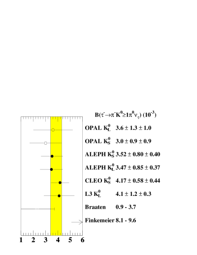
Figure 5: Branching ratios of the $\tau^{-}\rightarrow\pi^{-}\overline{\mathrm{K}}{}^{0}\nu_{\tau}$ and $\tau^{-}\rightarrow\pi^{-}\overline{\mathrm{K}}{}^{0}\mbox{\small$[\geq 1\pi^{0}]$}\nu_{\tau}$ decays measured or calculated to date. The solid band is the average branching ratio of the OPAL, ALEPH, CLEO and L3 measurements [14, 16]. The $\tau^{-}\rightarrow\pi^{-}\overline{\mathrm{K}}{}^{0}\mbox{\small$[\geq 1\pi^{0}]$}\nu_{\tau}$ results include both the $\tau^{-}\rightarrow\pi^{-}\overline{\mathrm{K}}{}^{0}\pi^{0}\nu_{\tau}$ and $\tau^{-}\rightarrow\pi^{-}\overline{\mathrm{K}}{}^{0}\pi^{0}\pi^{0}\nu_{\tau}$ measurements (ALEPH) and inclusive results (OPAL,L3,CLEO). The theoretical estimates are shown for the $\tau^{-}\rightarrow\pi^{-}\overline{\mathrm{K}}{}^{0}\pi^{0}\nu_{\tau}$ decay mode only [17, 18]. The open points show the new OPAL results, the solid points other experimental results and the bounded lines show two theoretical predicted ranges of the branching fractions.

The branching ratios are compared with existing measurements and theoretical predictions in fig. 5 for the $\tau^{-}\rightarrow\pi^{-}\overline{\mathrm{K}}{}^{0}\nu_{\tau}$ and $\tau^{-}\rightarrow\pi^{-}\overline{\mathrm{K}}{}^{0}\mbox{\small$[\geq 1\pi^{0}]$}\nu_{\tau}$ decay modes [14, 16]. The solid band is the new average branching ratio of the OPAL, ALEPH, CLEO and L3 measurements. The results of this work are in good agreement with previous measurements.

The branching ratios of the decay modes are predicted from various theoretical models. The measurement of the decay fraction of the $\tau^{-}\rightarrow\pi^{-}\overline{\mathrm{K}}{}^{0}\nu_{\tau}$ decay agrees well with the range $(8.9-10.3)\times 10^{-3}$ estimated by Braaten et al. in [17] and falls in the range of $(6.6-9.6)\times 10^{-3}$ predicted by Finkemeier and Mirkes in [18]. The decay $\tau^{-}\rightarrow\pi^{-}\overline{\mathrm{K}}{}^{0}\mbox{\small$[\geq 1\pi^{0}]$}\nu_{\tau}$, assuming that the decay contains only one $\pi^{0}$, is predicted to be in the range of $(0.9-3.7)\times 10^{-3}$ from [17] and in the range of $(8.1-9.6)\times 10^{-3}$ from [18]. The $\tau^{-}\rightarrow\pi^{-}\overline{\mathrm{K}}{}^{0}\pi^{0}\nu_{\tau}$ branching ratio prediction by Finkemeier and Mirkes is significantly higher than the experimental results, however they argue that the widths of the $\mathrm{K}_{1}$ resonance [11] used in their calculation are unusually narrow and that increasing the $\mathrm{K}_{1}$ width would give a prediction that agrees with the experimental measurements [19].

The branching ratio of the $\tau^{-}\rightarrow\mathrm{K}^{-}\mathrm{K}{}^{0}{\mbox{\small$[\geq 0\pi^{0}]$}}\nu_{\tau}$ decay mode is the sum of the $\tau^{-}\rightarrow\mathrm{K}^{-}\mathrm{K}{}^{0}\nu_{\tau}$ and $\tau^{-}\rightarrow\mathrm{K}^{-}\mathrm{K}{}^{0}\pi^{0}\nu_{\tau}$ decay modes. The decay fraction agrees well with the estimated range $(2.4-4.0)\times 10^{-3}$ predicted by [17] and $(2.3-2.7)\times 10^{-3}$ predicted by [18].

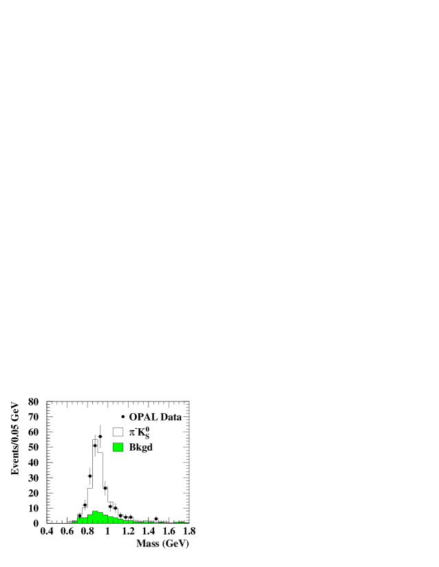
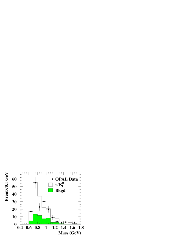
Figure 6: The $\overline{\mathrm{K}}{}^{0}_{\mathrm{S}}\pi^{-}$ and $\overline{\mathrm{K}}{}^{0}_{\mathrm{L}}\pi^{-}$ invariant mass spectra for the the decay channels $\tau^{-}\rightarrow\pi^{-}\overline{\mathrm{K}}{}^{0}_{\mathrm{S}}\nu_{\tau}$ and $\tau^{-}\rightarrow\pi^{-}\overline{\mathrm{K}}{}^{0}_{\mathrm{L}}\nu_{\tau}$, respectively.

The $\tau^{-}\rightarrow\pi^{-}\overline{\mathrm{K}}{}^{0}\nu_{\tau}$ decay mode is assumed to be dominated by the $\mathrm{K}^{*}(892)^{-}$ resonance. This can be observed from the $\pi^{-}\mathrm{\overline{K}^{0}}$ invariant mass distributions shown in fig. 6, for the decay modes $\tau^{-}\rightarrow\pi^{-}\overline{\mathrm{K}}{}^{0}_{\mathrm{S}}\nu_{\tau}$ and $\tau^{-}\rightarrow\pi^{-}\overline{\mathrm{K}}{}^{0}_{\mathrm{L}}\nu_{\tau}$, respectively. Assuming that the $\tau^{-}\rightarrow\pi^{-}\overline{\mathrm{K}}{}^{0}\nu_{\tau}$ decay mode proceeds entirely through the $\mathrm{K}^{*}(892)^{-}$ resonance, then using isospin invariance the branching ratio of the $\tau^{-}\rightarrow\mathrm{K}^{*}(892)^{-}\nu_{\tau}$ decay mode is calculated to be $0.0140\pm 0.0013$. This value is consistent with the current world average $0.0128\pm 0.0008$ [11].

Finally, the ratio of the decay constants $f_{\rho}$ and $f_{\mathrm{K}^{*}}$ can be estimated using the $\tau^{-}\rightarrow\mathrm{K}^{*}(892)^{-}\nu_{\tau}$ branching ratio and the OPAL $\tau^{-}\rightarrow\mathrm{h}^{-}\pi^{0}\nu_{\tau}$ branching ratio of $0.2589\pm 0.0034$ [7]. The $\tau^{-}\rightarrow\mathrm{h}^{-}\pi^{0}\nu_{\tau}$ decay mode is the sum of the decay modes $\tau^{-}\rightarrow\pi^{-}\pi^{0}\nu_{\tau}$ and $\tau^{-}\rightarrow\mathrm{K^{-}}\pi^{0}\nu_{\tau}$. The branching ratio of the $\tau$ to the final state $\mathrm{K^{-}}\pi^{0}\nu_{\tau}$ is calculated to be $(4.67\pm 0.42)\times 10^{-3}$ using isospin invariance and the $\tau^{-}\rightarrow\pi^{-}\overline{\mathrm{K}}{}^{0}\nu_{\tau}$ branching ratio. Consequently, $B(\tau^{-}\rightarrow\pi^{-}\pi^{0}\nu_{\tau})$ is derived to be $0.2543\pm 0.0034$. Using these results, $\tan\theta_{c}=0.227$ for the Cabibbo angle and the particle masses from [11], the decay constant ratio

$$\frac{f_{\rho}}{f_{\mathrm{K}^{*}}}=\tan\theta_{c}\sqrt{\frac{B(\tau^{-}\rightarrow\rho^{-}\nu_{\tau})}{B(\tau^{-}\rightarrow\mathrm{K}^{*}(892)^{-}\nu_{\tau})}}\left(\frac{m^{2}_{\tau}-m^{2}_{\mathrm{K}^{*}}}{m^{2}_{\tau}-m^{2}_{\rho}}\right)\sqrt{\frac{m^{2}_{\tau}+2m^{2}_{\mathrm{K}^{*}}}{m^{2}_{\tau}+2m^{2}_{\rho}}}=0.93\pm 0.05$$

is obtained. The error is dominated by the uncertainties on the branching ratios. The recent result from ALEPH [13], $0.94\pm 0.03$, agrees well with the new OPAL result. Finally, this ratio has been predicted by Oneda [20] using the Das-Mathur-Okubo sum rule relations [21] between the spectral functions based on assumptions of $SU(3)_{f}$ symmetry. At the $SU(3)_{f}$ symmetry limit ($m_{\mathrm{u}}=m_{\mathrm{d}}=m_{\mathrm{s}}$), the decay constant ratio is expected to be unity, $f_{\rho}=f_{\mathrm{K}^{*}}$. In the asymptotic $SU(3)_{f}$ symmetry limit at high energies, Oneda predicts that $f_{\rho}/f_{\mathrm{K}^{*}}=m_{\rho}/m_{\mathrm{K}^{*}}=0.86$.

Table 1: Signal efficiencies for each selection relative to selecting a $\mathrm{K^{0}}$. The errors on these efficiencies are based on Monte Carlo statistics only. The first column lists the three selection classes. The three remaining columns give the Monte Carlo selection efficiency for a decay of the indicated type passing that selection classification.

Selection	Selection efficiency from MC (%)
	$\tau^{-}\rightarrow\pi^{-}\overline{\mathrm{K}}{}^{0}\nu_{\tau}$	$\tau^{-}\rightarrow\pi^{-}\overline{\mathrm{K}}{}^{0}\mbox{\small$[\geq 1\pi^{0}]$}\nu_{\tau}$	$\tau^{-}\rightarrow\mathrm{K}^{-}\mathrm{K}{}^{0}{\mbox{\small$[\geq 0\pi^{0}]$}}\nu_{\tau}$
$\mathrm{K}{}^{0}_{\mathrm{L}}$ sample
$\pi^{-}\overline{\mathrm{K}}{}^{0}$	$7.36\pm 0.18$	$0.81\pm 0.09$	$0.28\pm 0.06$
$\pi^{-}\overline{\mathrm{K}}{}^{0}[\geq 1\pi^{0}]$	$1.05\pm 0.07$	$3.60\pm 0.19$	$0.08\pm 0.03$
$\mathrm{K}^{-}\mathrm{K}{}^{0}[\geq 0\pi^{0}]$	$0.43\pm 0.05$	$0.19\pm 0.04$	$3.53\pm 0.21$
$\mathrm{K}{}^{0}_{\mathrm{S}}$ sample
$\pi^{-}\overline{\mathrm{K}}{}^{0}$	$8.94\pm 0.18$	$2.88\pm 0.18$	$1.46\pm 0.13$
$\pi^{-}\overline{\mathrm{K}}{}^{0}[\geq 1\pi^{0}]$	$0.48\pm 0.05$	$5.32\pm 0.24$	$0.27\pm 0.06$
$\mathrm{K}^{-}\mathrm{K}{}^{0}[\geq 0\pi^{0}]$	$0.99\pm 0.07$	$0.93\pm 0.10$	$8.44\pm 0.29$

Table 2: Systematic errors on the branching ratios.

	Branching ratio systematic errors ($\times 10^{-3}$) for the $\mathrm{K}{}^{0}_{\mathrm{L}}$ selection
	$B(\tau^{-}\rightarrow\pi^{-}\overline{\mathrm{K}}{}^{0}\nu_{\tau})$	$B(\tau^{-}\rightarrow\pi^{-}\overline{\mathrm{K}}{}^{0}\mbox{\small$[\geq 1\pi^{0}]$}\nu_{\tau})$	$B(\tau^{-}\rightarrow\mathrm{K}^{-}\mathrm{K}{}^{0}{\mbox{\small$[\geq 0\pi^{0}]$}}\nu_{\tau})$
MC statistics	0.24	0.28	0.24
Bias factor	0.14	0.05	0.05
$\mathrm{K}{}^{0}_{\mathrm{L}}$ efficiency	0.40	0.68	0.42
Background	0.29	0.50	0.31
${\mathrm{d}}E/{\mathrm{d}}x$ modelling	0.21	0.11	0.33
$\pi^{0}$ efficiency	$0.14$	$0.27$	0.00
MC modelling	$0.00$	$0.39$	$0.17$
Total	0.62	1.02	0.68
	Branching ratio systematic errors ($\times 10^{-3}$) for the $\mathrm{K}{}^{0}_{\mathrm{S}}$ selection
	$B(\tau^{-}\rightarrow\pi^{-}\overline{\mathrm{K}}{}^{0}\nu_{\tau})$	$B(\tau^{-}\rightarrow\pi^{-}\overline{\mathrm{K}}{}^{0}\mbox{\small$[\geq 1\pi^{0}]$}\nu_{\tau})$	$B(\tau^{-}\rightarrow\mathrm{K}^{-}\mathrm{K}{}^{0}{\mbox{\small$[\geq 0\pi^{0}]$}}\nu_{\tau})$
MC statistics	$0.23$	$0.17$	$0.15$
Bias factor	$0.10$	$0.09$	$0.07$
$\mathrm{K}{}^{0}_{\mathrm{S}}$ efficiency	$0.46$	$0.66$	$0.18$
Background	$0.40$	$0.44$	$0.21$
${\mathrm{d}}E/{\mathrm{d}}x$ modelling	$0.26$	$0.10$	$0.32$
$\pi^{0}$ efficiency	$0.22$	$0.22$	$0.00$
MC modelling	$0.00$	$0.31$	$0.16$
Total	$0.74$	$0.91$	$0.48$

References

-
[1]
OPAL Collaboration, K. Ahmet et al.,
Nucl. Instr. and Meth. A305 (1991) 275;
P.P. Allport et al., Nucl. Instr. and Meth. A324 (1993) 34;
P.P. Allport et al., Nucl. Instr. and Meth. A346 (1994) 476. -
[2]
M. Hauschild et al., Nucl. Instr. and Meth. A314 (1992) 74;
O. Biebel et al., Nucl. Instr. and Meth. A323 (1992) 169;
M. Hauschild, Nucl. Instr. and Meth. A379 (1996) 436. - [3] S. Jadach, B.F.L. Ward, and Z. Wa̧s, Comp. Phys. Comm. 79 (1994) 503.
- [4] S. Jadach et al., Comp. Phys. Comm. 76 (1993) 361.
- [5] J. Allison et al., Nucl. Inst. and Meth. A317 (1992) 47.
- [6] OPAL Collaboration, G. Alexander et al., Phys. Lett. B369 (1996) 163.
- [7] OPAL Collaboration, K. Ackerstaff et al., Eur. Phys. J. C4 (1998) 193.
- [8] OPAL Collaboration, K. Ackerstaff et al., Eur. Phys. J. C8 (1999) 183.
- [9] OPAL Collaboration, R. Akers et al., Z. Phys. C67 (1995) 389.
- [10] OPAL Collaboration, G. Alexander et al., Z. Phys. C70 (1996) 357.
- [11] Particle Data Group, C. Caso et al., Eur. Phys. J. C3 (1998) 1.
- [12] M. Lefebvre, R.K. Keeler, R. Sobie and J. White, Propagation of Errors for Matrix Inversion, hep-ex/9909031, Submitted to Nucl. Inst. and Meth.
- [13] ALEPH Collaboration, R. Barate et al., Study of Tau Decays Involving Kaons, Spectral Functions and Determination of the Strange Quark Mass, CERN-EP/99-026.
- [14] ALEPH Collaboration, R. Barate et al., Eur. Phys. J., C10 (1999) 1.
- [15] OPAL Collaboration, G. Abbiendi et al., A Study of three Prong Tau Decays with Charged Kaons, CERN-EP/99-095.
-
[16]
ALEPH Collaboration, R. Barate et al., Eur. Phys. J., C4 (1998) 29;
L3 Collaboration, M. Acciarri et al., Phys. Lett. B352 (1995) 487;
CLEO Collaboration, T.E. Coan et al., Phys. Rev. D53 (1996) 6037. - [17] E. Braaten, R. Oakes and S. Tse, Int. J. Mod. Phys., A5 (1990) 2737.
- [18] M. Finkemeier and E. Mirkes, Z.Phys., C69 (1996) 243.
- [19] M. Finkemeier, J.H. Kühn and E. Mirkes, Nucl. Phys. Proc. Suppl. C55 (1997) 169.
-
[20]
S. Oneda, Phys. Rev. D35 (1987) 397;
T. Matsuda and S. Oneda, Phys. Rev. 171 (1968) 1743. -
[21]
T. Das, V.S. Mathur and S. Okubo, Phys. Rev. Lett. 18
(1967) 761;
T. Das, V.S. Mathur and S. Okubo, Phys. Rev. Lett. 19 (1967) 859.