Abstract

We present an algorithm which allows a fast numerical computation of Feldman-Cousins confidence intervals for Poisson processes, even when the number of background events is relatively large. This algorithm incorporates an appropriate treatment of the singularities that arise as a consequence of the discreteness of the variable.

PACS: 02.70.-c, 06.20.Dk, 29.85.+c

1 Introduction

In physics there are many situations where the outcome of an experiment is a positive integer number with a Poisson distribution. This is the case for instance of the number of events of a certain type produced in high energy collisions. The statistical analysis of these processes is a difficult task when the result obtained is in the limit of the sensitivity of the experiment. In general, the number of events $n_{0}$ obtained in an experiment consists of background events with known mean $b$ and signal events, whose mean $\mu$ is the quantity that we want to determine. The problem arises when the number of events obtained $n_{0}$ is significantly lower than the background expected $b$. This happens in some experiments on neutrino oscillations, for instance in the KARMEN 2 experiment [1].

Usually, after performing an experiment, one decides whether to give the results on the unknown parameter $\mu$ in the form of a central confidence interval or an upper bound. This decision (called ‘flip-flopping’) is based on the data and, as has been shown by Feldman and Cousins [2], introduces a bias that may cause that the intervals cover the true value $\mu$ with a smaller frequency than the stated confidence level. To solve this and other problems, they introduce a new ordering principle that unifies the treatment of central confidence intervals and upper limits. This is possible because the Neyman construction of confidence intervals [3] allows the choice of the ordering principle with which the intervals are constructed. Typical choices lead to the construction of either central intervals or upper confidence limits. The choice of Feldman and Cousins gives intervals that are two-sided or upper limits depending on the result of the experiment and not on the choice of the experimentalist. These intervals avoid the undercoverage caused by ‘flip-flopping’ and are non-empty in all cases. Some variants of their method have been also proposed [4, 5].

To consider the Feldman-Cousins confidence intervals as an alternative to standard intervals, in practice one needs to calculate these intervals for arbitrary $n_{0}$ and $b$. The Tables provided in Ref. [2], for $n_{0}\leq 20$, $b\leq 15$, are sufficient for small luminosity/statistics experiments, but for higher luminosities in general $b$ and $n_{0}$ are larger. One possibility is to extend these Tables using the same systematic computational method of Ref. [2], whose speed is not optimized and consumes a lot of time. More convenient is to develop a program which takes $n_{0}$ and $b$ as inputs and gives as output the confidence interval, requiring a minimal number of calculations. This is what is done here. The program can be used either directly to compute the confidence interval for given $n_{0}$ and $b$ or in conjunction with other routines. This is especially useful, for instance to calculate expected limits from rare high energy processes for different values of the center of mass energy or the collider luminosity, which is the case that we were primarily interested in.

In the following we introduce a procedure to compute the Feldman-Cousins intervals in an efficient way for arbitrary $n_{0}$ and $b$, in principle only limited by the machine precision. In Section 2 we review Neyman’s construction of the confidence intervals for a Poisson variable, emphasizing some points that simplify the numerical calculation. Section 3 is more technical and devoted to explain in depth how to translate this method for the computer calculation. In Section 4 we present our results. The FORTRAN implementation of the algorithm is given in the Appendix. Other implementations in C and Mathematica [6] (about 100 times slower than the FORTRAN version) can be obtained from the author.

2 Construction of the confidence intervals

The probability to observe $n$ events in a Poisson process consisting of signal events with unknown mean $\mu$ and background events with known mean $b$ is given by the formula

$$P(n\,|\,\mu;b)=\frac{(\mu+b)^{n}}{n!}e^{-(\mu+b)}\,,$$ (1)

with $n,\mu,b\geq 0$, and $n$ restricted to integer values. The construction of the confidence intervals on the unknown variable $\mu$ follows Neyman’s method of the confidence belts.

The first step in this procedure is to construct, for a fixed value of $b$ and for different values of $\mu$, the confidence intervals $[n_{1}(\mu;b),n_{2}(\mu;b)]$ such that the probability to obtain a result between $n_{1}$ and $n_{2}$ is greater or equal than $\alpha$, the confidence level (C. L.),

$$P(n\;\epsilon\;[n_{1},n_{2}]\,|\,\mu;b)=\sum_{n=n_{1}}^{n_{2}}P(n\,|\,\mu;b)\geq\alpha\,.$$ (2)

It is worth to note that for the more general case of a continuous variable $x$ the intervals $[x_{1}(\mu;b),x_{2}(\mu;b)]$ satisfy $P(n\;\epsilon\;[x_{1},x_{2}]\,|\,\mu;b)=\alpha$. For a discrete variable $n$ it is not possible to obtain the exact equality, and to avoid undercoverage it is replaced by the inequality in Eq. (2).

The choice of the intervals $[n_{1},n_{2}]$ is not unique, and determines the type of confidence intervals on $\mu$ that are constructed. The most common choices are $n_{2}=\infty$, $P(n\leq n_{1}\,|\,\mu;b)\leq 1-\alpha$, which gives upper confidence bounds, and $P(n\leq n_{1}\,|\,\mu;b)\leq(1-\alpha)/2$, $P(n\geq n_{2}\,|\,\mu;b)\leq(1-\alpha)/2$ which leads to central confidence intervals. The prescription of Ref. [2] is based on a likelihood ratio $R$, constructed as follows.

1. For any values of $b$ and $n$, one considers which value of $\mu$ would maximize the probability $P(n\,|\,\mu;b)$ . It is straightforward to find that for $n\geq 1$, $P(n\,|\,\mu;b)$ considered as a function of $\mu$ grows for $\mu<n-b$, has a maximum at $\mu=n-b$ and decreases for $\mu>n-b$. As $\mu$ is restricted to lie in the positive real axis, if $n\geq b$ the maximum is $\mu=n-b$, otherwise the maximum is $\mu=0$. In the case $n=0$ the maximum is also $\mu=0$, so we define

   $$\mu_{\mathrm{best}}(n;b)=\max\{0,n-b\}$$ (3)

   as the value which maximizes $P(n\,|\,\mu;b)$.

2. Then, for any value of $\mu$ we consider the quantity $R(n;\mu,b)$ defined as

   $$R(n;\mu,b)=\frac{P(n\,|\,\mu;b)}{P(n\,|\,\mu_{\mathrm{best}}(n;b);b)}\leq 1\,,$$ (4)

   on which the Feldman-Cousins ordering principle is based. To construct the interval $[n_{1}(\mu;b),n_{2}(\mu;b)]$, for each value of $\mu$ (and fixed $b$) one takes values of $n$ with decreasing $R(n;\mu,b)$, summing up their probabilities $P(n\,|\,\mu;b)$ until the total equals or exceeds the C. L. desired $\alpha$. Thus the interval $[n_{1},n_{2}]$ is the set of values of $n$ necessary to satisfy the inequality in Eq. (2), taken with the largest $R(n;\mu,b)$.

The simplicity of this prescription allows a fast computer implementation. Instead of generating a large table of values for $n$ and taking those with the largest $R$, we can directly find these values and add them successively to construct the interval. (This is difficult to do with the more involved prescriptions of Refs. [4, 5].) For this purpose we will examine the behaviour of $R$. If we consider

$$R(x;\mu,b)=\frac{(\mu+b)^{x}e^{-(\mu+b)}}{(\mu_{\mathrm{best}}(x;b)+b)^{x}e^{-(\mu_{\mathrm{best}}(x;b)+b)}}$$ (5)

as a function of the continous variable $x$, we can look for its maximum. Let us first consider $\mu\neq 0$, $b\neq 0$. For $x$ sufficiently small, $\mu_{\mathrm{best}}(x;b)=0$ and $R(x;\mu,b)=(1+\mu/b)^{x}e^{-\mu}$ is increasing. For $x\geq b$, $\mu_{\mathrm{best}}(x;b)=x-b$ and $R(x;\mu,b)=(e(\mu+b)/x))^{x}e^{-(\mu+b)}$ grows for $x<\mu+b$, falls for $x>\mu+b$ and has a local maximum at $x=\mu+b$, which is then the global maximum. This is also true for $\mu\neq 0$, $b=0$. For $\mu=0$, $b\neq 0$ and $x<b$, $\mu_{\mathrm{best}}(x;b)=0$ and $R(x;0,b)=1$, its maximum possible value. For $x\geq b$, $R(x;0,b)=(b/x)^{x}e^{x-b}$ decreases with $x$. Hence the maximum is still $x=\mu+b$, although not unique. The only remaining case with $\mu=0$, $b=0$ in which the Poisson distribution is singular must be treated separately.

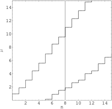
Figure 1: Confidence belt for $b=3$, with $\alpha=0.9$. The vertical line is drawn for $n_{0}=8$.

With this method, and for different values of $\mu$ ($b$ is fixed), one calculates the confidence intervals $[n_{1}(\mu;b),n_{2}(\mu;b)]$ obtaining a confidence belt like the one showed in Fig. 1 for $b=3$ and a C. L. of 0.9. To find the confidence interval $[\mu_{1},\mu_{2}]$ for a particular experimental value $n_{0}$, one draws a vertical line at $n=n_{0}$ and finds the maximum and minimum values of $\mu$ for which the line intersects the confidence belt. In Fig. 1 we observe that $\mu_{1}$ is the smallest $\mu$ such that $n_{2}(\mu;b)=n_{0}$, whereas $\mu_{2}$ is the largest $\mu$ for which $n_{1}(\mu;b)=n_{0}$.

3 Implementation

Let us explain how the method described in Section 2 is made suitable for the evaluation in a computer. For the calculations we use the FORTRAN version of the program compiled with fort77 under Linux on a Pentium III-450 (compiled with g77 the program runs about 25% slower), and for the plots we also use the Mathematica version.

The first problem in the practical realization of the Neyman construction is that, for large $b$, $n$ or $\mu$, the factors of the Poisson probability formula in Eq. (1) can overflow (or underflow) the computer capacity in intermediate calculations. The factor $(\mu+b)^{n}$ may be very large, for instance $54^{178}$ is larger the biggest double precision real number in the FORTRAN compiler used, approximately $10^{308}$. However, the exponential factor in Eq. (1) compensates for it in the final result. For $\mu+b+n>230$ we evaluate P using the expression

$$P(n\,|\,\mu;b)=e^{-\mu}\prod_{i=1}^{n}\left(\frac{\mu+b}{i}\right)e^{-b}\,,$$ (6)

with the product calculated factor by factor. This extends the allowed size of the parameters of our program, with the disadvantage of a larger computing time. For $\mu+b+n\leq 230$ the factor $(\mu+b)^{n}$ is not too large, and can be directly calculated. In this case the factorials up to $170!\sim 10^{307}$ are calculated at the beginning of the main program and stored in the array fact to save time, whereas for $n>170$ the expression of the Poisson formula is divided by $\prod_{i=1}^{n}i$ factor by factor.

The quantity $R$ in Eq. (4) is a ratio of probabilities and can be computed without any problem cancelling out the common factors and defining a function R. (Defining $\mu_{\mathrm{best}}$ as DIM(FLOAT(n),b) instead of MAX(0d0,FLOAT(n)-b) as we do would not have improved the speed significantly.)

The core of the algorithm is the subroutine NRANGE, used to calculate the confidence intervals $[n_{1}(\mu;b),n_{2}(\mu;b)]$ for arbitrary $\mu$ and $b$. Its arguments are the variables rmu ($\mu$), b and the confidence level desired CL. The output n1 and n2 is given in a COMMON block, together with a variable CLac, the C. L. finally achieved (in general it is greater than CL) which is useful for other purposes. The discussion in the last Section simplifies the implementation of the algorithm considerably, because we have found that the values of $n$ that maximize $R(n;\mu,b)$ concentrate around $\mu+b$. This improves the speed by an order of magnitude for large values of the parameters, since we do not need to calculate a large table $(n,P(n),R(n))$ and sort it. Instead, we know the maximum R is one of the two integers nearest to $\mu+b$. We begin with n1=INT(rmu+b), n2=n1+1. If R(n1,rmu,b) is larger than R(n2,rmu,b) we take n1, decrease n1 and add P(n1,rmu,b) to CLac. Otherwise, we take n2, increase n2 and add P(n2,rmu,b) to CLac. Repeating this until CLac is greater than CL and taking into account that n1 must be greater than zero we obtain the desired interval $[n_{1},n_{2}]$. The singular case $\mu=b=0$ is treated separately. With the Mathematica version of this subroutine we can plot confidence belts like that in Fig. 1.

The calculation of the confidence interval $[\mu_{1},\mu_{2}]$ is done using two funcions RMU1(n,b,CL) and RMU2(n,b,CL), where n is the experimental number of events. We discuss them in turn.

As we see in Fig. 1, the lower limit $\mu_{1}$ is the minimum value of $\mu$ such that $n_{2}(\mu;b)=n_{0}$. Within our framework, the calculation is done looking for the minimum rmu such that n2 calculated with NRANGE(rmu,b,CL) equals n. The search is done with the bisection method. Starting with the limits rmumin=0d0, rmumax=FLOAT(n)-b+1d0 (RMU1 must be between these two values) we calculate the midpoint of the interval, rmumed, and NRANGE(rmumed,b,CL). If n2 is greater or equal than n, we move rmumax to rmumed, otherwise we move rmumin to rmumed. This is repeated until the length of the interval is smaller than the desired precision delta, which we take as the maximum of 0.01 and 0.0005 times the background $b$. We summarize the algorithm in Fig. 2.

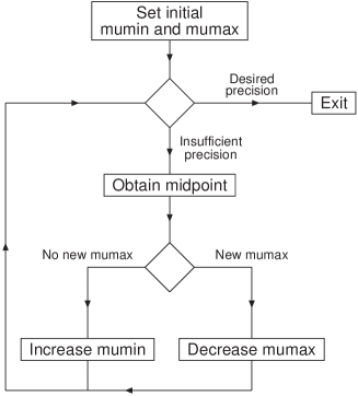
Figure 2: Flux diagram for the calculation of RMU1.

In principle the calculation of RMU2 would follow an analogous procedure. However, in this case we find an extra problem. Except for a few cases with small $b$, the confidence belt is not as simple as in Fig. 1 but displays a more elaborated structure as can be seen in the example of Fig. 3.

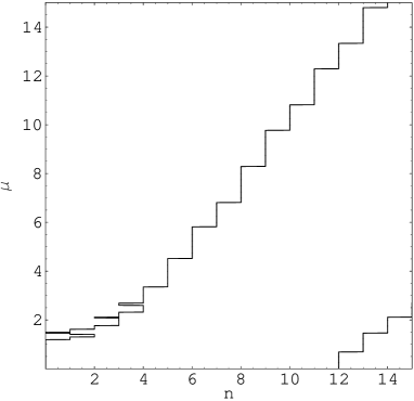
Figure 3: Confidence belt for $b=7$, with $\alpha=0.95$.

The fact that $n_{1}(\mu;b)$ is not a monotonic function of $\mu$ is due to the discreteness of $n$. This causes that the set of $\mu$ values for which the vertical line at $n=n_{0}$ intersects the belt is not connected for $n_{0}=0-4$. The effect is relevant since the upper limit $\mu_{2}$ is defined as the largest $\mu$ for which $n_{1}(\mu;b)=n_{0}$. Thus a modification of the algorithm is required not to miss the small wedges in the function.

For $n\geq b$ the behaviour is as expected and we can use the same algorithm as for $\mu_{1}$. We have checked values of $b$ between 0 and 50 and have found that for $n\geq b$ the function $n_{1}(\mu;b)$ does not have any singularity, so in this case we can safely adapt the routine RMU1. We look for the maximum rmu such that n1 calculated with NRANGE(rmu,b,CL) equals n. The search is again done with the bisection method. We start with the initial values rmumin=MAX(0d0,FLOAT(n)-b), rmumax=3d0*SQRT(FLOAT(n)+b+1d0). (If rmumax is not sufficiently large, we increment it in steps of SQRT(FLOAT(n)+b+1d0).) We calculate the midpoint of the interval, rmumed, and calculate NRANGE(rmumed,b,CL). If n1 is lower or equal to n, we move rmumin to rmumed, otherwise we move rmumax to rmumed. This is repeated until the length of the interval is smaller than the desired presision delta.

For $n<b$ we sample the interval for possible singularities, which consumes more time. This is done in three iterations with increasing number of points. To minimize the length of the interval and optimize the density of the sampling, we take rmumin=MAX(0d0,FLOAT(n)-b) and increase it in steps of 1 while n1 is lower or equal to n. As the upper limit we take rmumax=3d0*SQRT(FLOAT(n)+b+1d0), sufficiently high so that the initial interval contains all the singularities for a C. L. of 0.99 or less.

In the first step we divide the interval between rmumin and rmumax in 10 parts and check if any of the points selected has n1 lower or equal to n. If it is so, we change rmumin to the largest of them (this is always safe) and start again with this new rmumin. This first sampling with a small number of points finds wedges like those for $n=1,3$ in Fig. 3 and saves a lot of computing time. The narrow wedges at $n=0,2$ require more dense samplings.

If the points calculated have n1 greater than n, we check the upper half of the interval for singularities. The second iteration divides the upper half in 20 parts and checks 19 points. If it finds any singular point with n1 lower or equal to n, it changes rmumin and starts again at the first step. If not, the third iteration divides the upper half in 500 parts. If a singular point is found, it changes rmumin and starts the first step. If not, unless some kind of singular behavior is found (in which case a fourth sampling with 5000 points is performed) it is assumed that there do not exist singulariries and rmumax is changed.

An additional speed improvement is implemented: if in the second or third iterations the density of points is sufficiently high (the points are closer than stepmin), the number of points is decreased and no more iterations are performed. The flux diagram of RMU2 is shown in Fig. 4.

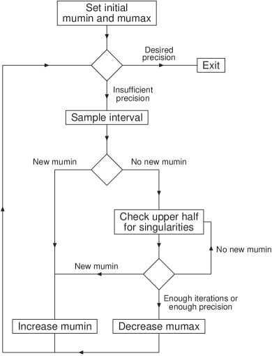
Figure 4: Flux diagram for the calculation of RMU2.

To simplify changing the parameters of this routine, the number of iterations and their respective number of points are stored in the variables maxit and maxdivs. The calculation for $n\geq b$ is done with the same function with maxdivs(1)=2 and only the first iteration.

One may notice that some upper limits obtained with RMU2 are different from those quoted in Ref. [2]. This is again a consequence of the discreteness of $n$. The upper limit $\mu_{2}$ for $n_{0}$ fixed is not always a decreasing function of $b$ (dotted lines in Fig. 5.) This behaviour is corrected in Ref. [2] forcing the function to be nonincreasing, calculating the upper limit $\mu_{2}$ from $b=25$ to $b=0$ in steps of $-0.001$. The corrected value is then the maximum of $\mu_{2}(n_{0},x)$ for $x\geq b$. Some people, however, find this ad hoc correction questionable [4]. At any rate we could also follow this procedure getting the same values of Ref. [2] and the solid line in Fig. 5. This requires a very long calculation (25000 different values of $b$), for instance the time to calculate the $n_{0}=0$ line is 34 m 27 s.

Figure 5: Dependence of $\mu_{2}$ on the expected background $b$ for fixed $n_{0}$. The solid and dotted lines are obtained with and without correction, respectively.

Of course, to obtain $\mu_{2}$ for a particular $b$ it is not necessary to calculate the whole interval $[b,20]$ and it is enough to consider approximately $[b,b+1]$. For this purpose we use the function RMU2c. This routine examines the behaviour of RMU2 in the interval $[b,b+1]$ and corrects the value if necessary. The adjacent maxima that can be seen in Fig. 5 are found with the simple golden section search of Ref. [7]. (Other more sophisticated methods offer no advantage since the function does not seem to be differentiable at the maximum.) The initial bracketing of the maximum is very delicate as can be also seen in this Figure. We do it examining RMU2(n,b1,CL) taking b1 with increments of 0.1 until RMU2 begins to grow, then in increments of 0.05 until it begins to decrease. Then the golden section method is applied to find the maximum with a precision of 0.001. This maximum is then compared to the value at b to take the largest value.

This method again brings a substantial speed improvement over the blind computation in steps of $-0.001$ in $b$, as we will see in next Section, Examining the behaviour of $\mu_{2}$ we have also found that the correction is not necessary in general for $n>b/2$ and the function RMU2 could be used directly. There are however some exceptions, for instance $n=10$, $b=14$ with a C. L. of 0.95. To be conservative, we will only use RMU2 when $n\geq b$.

4 Results

To obtain our results we use the same precision that is used in Ref. [2], a minimum step stepmin of 0.005 in $\mu$ and an accuracy of 0.01 in the upper and lower limits of the confidence intervals. To calculate the limits in their Tables II–IX including the singular cases it is enough to consider in the third iteration maxdivs(3)=100 for confidence levels of $68.7\%$, $90\%$ and $95\%$, and maxdivs(3)=300 for a C. L. of $99\%$. For better comparison we use maxdivs(3)=500 as we do in the rest of the calculations to ensure that all singularities are found. The running time is summarized in Table 1.

C. L.	$t_{1}$	$t_{2}$
68.7%	4.1 s	1 m 9.0 s
90%	6.1 s	1 m 28.6 s
95%	6.8 s	1 m 36.8 s
99%	7.9 s	1 m 57.4 s

Table 1: Time spent in the calculation of the confidence intervals for $n_{0}\leq 20$ and $b\leq 15$, with RMU2 ($t_{1}$) and with RMU2c ($t_{2}$).

To check if our algorithm in fact handles large numbers efficiently we measure the time spent to calculate the upper limit $\mu_{2}$ with RMU2 for $n_{0}=b$ between 0 and 200, obtaining the solid line in Fig. 6. We can also use RMU2c forcing the program to look for unexisting spurious maxima in $b$ (and hence also for singularities with maxdivs(3)=500) obtaining the dotted line.

Figure 6: Time required to calculate the upper limit $\mu_{2}$ with the function RMU2 ($t_{1}$) and with RMU2c forcing to look for adjacent maxima ($t_{2}$) as explained in the text.

It is amazing to observe that the computing time not only does not grow quickly with $b$ as it could be expected, but remains almost constant for $b<75$. This is achieved with (i) a fast algorithm to find the singularities if they exist, (ii) the optimization of NRANGE to calculate only the data really needed, and (iii) the calculation of the factorials up to $170!$ at the beginning of the program. For $b\geq 75$ rmu+b+FLOAT(n) is sometimes larger than 230 and the time required begins to grow linearly with $b$ after the gap between 75 and 100, as can be observed in the Figure.

Acknowledgements

I thank F. del Aguila for discussions and for a critical reading of the manuscript. This work was partially supported by CICYT under contract AEN96–1672 and by the Junta de Andalucía, FQM101.

Appendix A Appendix

      PROGRAM DEMO
      IMPLICIT REAL*8 (A-H,O-Z)
      DIMENSION FACT(0:170)
      COMMON /range/ n1,n2,CLac
      COMMON /factorial/ FACT
      DATA CL /0.99d0/

      FACT(0)=1d0                           ! FACT initialization
      DO i=1,170
        FACT(i)=FACT(i-1)*DFLOAT(i)
      ENDDO

C     CALCULATION OF TABLES VIII, IX OF REF[2]

      DO b=0d0,4d0,0.5d0
        DO n=0,20
          PRINT 100,n,b,RMU1(n,b,CL),RMU2c(n,b,CL)
        ENDDO
      ENDDO
      DO b=5d0,15d0,1d0
        DO n=0,20
          PRINT 100,n,b,RMU1(n,b,CL),RMU2c(n,b,CL)
        ENDDO
      ENDDO
      STOP

100   FORMAT (’n = ’,I2,’, b = ’,F4.1,’ -> [’,F6.2,’,’,F6.2,’]’)
      END


      DOUBLE PRECISION FUNCTION P(n,rmu,b)
      IMPLICIT REAL*8 (A-H,O-Z)
      DIMENSION FACT(0:170)
      COMMON /factorial/ FACT
      IF ((rmu .EQ. 0d0) .AND. (b .EQ. 0d0)) THEN    ! These lines
        P=0                                          ! are not
        IF (n .EQ. 0) P=1                            ! needed if P is
        RETURN                                       ! only called
      ENDIF                                          ! from NRANGE
      IF (rmu+b+FLOAT(n) .LE. 230d0) THEN
        P=(rmu+b)**n*EXP(-rmu-b)
        IF (n .LE. 170) THEN
          P=P/FACT(n)
        ELSE
          P=P/FACT(170)    ! This is not normally used because for
          DO i=171,n       ! n > 170 rmu+b+FLOAT(n) will be larger
            P=P/FLOAT(i)   ! than 230
          ENDDO
        ENDIF
      ELSE
        P=EXP(-rmu)
        DO i=1,n
          P=P*(rmu+b)/FLOAT(i)
        ENDDO
        P=P*EXP(-b)
      ENDIF
      RETURN
      END

      DOUBLE PRECISION FUNCTION R(n,rmu,b)
      IMPLICIT REAL*8 (A-H,O-Z)
      IF (n .LT. 0) THEN
        R=0d0
        RETURN
      ENDIF
      R=EXP(MAX(0d0,FLOAT(n)-b)-rmu)
      IF (n .GT. 0) R=R*((rmu+b)/(MAX(0d0,FLOAT(n)-b)+b))**n
      RETURN
      END


      SUBROUTINE NRANGE(rmu,b,CL)
      IMPLICIT REAL*8 (A-H,O-Z)
      COMMON /range/ n1,n2,CLac  ! CLac for future use
      IF ((rmu .EQ. 0d0) .AND. (b .EQ. 0d0)) THEN
        n1=0d0                   ! Special case
        n2=0d0
        RETURN
      ENDIF
      n1=INT(rmu+b)              ! The maximum R is between
      n2=n1+1                    ! these values
      r1=R(n1,rmu,b)
      r2=R(n2,rmu,b)
      CLac=0d0
      DO WHILE ((CLac .LT. CL) .AND. (n1 .GE. 0))
        IF (r1 .GT. r2) THEN
          CLac=CLac+P(n1,rmu,b)
          n1=n1-1
          r1=R(n1,rmu,b)
        ELSE
          CLac=CLac+P(n2,rmu,b)
          n2=n2+1
          r2=R(n2,rmu,b)
        ENDIF
      ENDDO
      DO WHILE (CLac .LT. CL)    ! No need to calculate R
        CLac=CLac+P(n2,rmu,b)
        n2=n2+1
      ENDDO
      n1=n1+1
      n2=n2-1
      RETURN
      END


      DOUBLE PRECISION FUNCTION RMU1(n,b,CL)
      IMPLICIT REAL*8 (A-H,O-Z)
      COMMON /range/ n1,n2,CLac
      CALL NRANGE(0d0,b,CL)
      IF (n2 .GE. n) THEN
        RMU1=0d0                                ! Special case
        RETURN
      ENDIF
      rmumin=0d0
      rmumax=FLOAT(n)-b+1d0
      delta=MAX(0.01d0,0.0005d0*b)
      DO WHILE ((rmumax-rmumin) .GE. delta)     ! Bisection method
        rmumed=(rmumin+rmumax)/2d0
        CALL NRANGE(rmumed,b,CL)
        IF (n2 .GE. n) THEN
          rmumax=rmumed
        ELSE
          rmumin=rmumed
        ENDIF
      ENDDO
      RMU1=(rmumin+rmumax)/2d0
      RETURN
      END


      DOUBLE PRECISION FUNCTION RMU2(n,b,CL)
      IMPLICIT REAL*8 (A-H,O-Z)
      DIMENSION maxdivs(4)
      LOGICAL safe,safenow,sing,changemin
      COMMON /range/ n1,n2,CLac
      DATA maxdivs /10,20,500,5000/
      maxit=4
      stepmin=0.005d0
      rmumin=MAX(0d0,FLOAT(n)-b)
      CALL NRANGE(rmumin,b,CL)
      IF (FLOAT(n) .LT. b) THEN
        DO WHILE (n1 .LE. n)          ! Take lower limit
          rmumin=rmumin+1d0           ! as high as possible
          CALL NRANGE(rmumin,b,CL)
        ENDDO
        rmumin=rmumin-1d0
        safe=.FALSE.
      ELSE
        maxdivs(1)=2                  ! Use bisection method when
        safe=.TRUE.                   ! there aren’t sing.
      ENDIF
      rmumax=3d0*SQRT(FLOAT(n)+b+1d0) ! Large enough for most purposes
      CALL NRANGE(rmumax,b,CL)
      DO WHILE (n1 .LE. n)            ! If not, increase it
        rmumax=rmumax+SQRT(FLOAT(n)+b+1d0)
        CALL NRANGE(rmumax,b,CL)
      ENDDO
      delta=MAX(0.01d0,0.0005d0*b)
      DO WHILE ((rmumax-rmumin) .GE. delta)
        step=(rmumax-rmumin)/FLOAT(maxdivs(1))
        rmumin2=rmumin
        DO i=1,maxdivs(1)-1
          CALL NRANGE(rmumin+FLOAT(i)*step,b,CL)
          IF (n1 .LE. n) rmumin2=rmumin+FLOAT(i)*step
        ENDDO
        IF (rmumin2 .GT. rmumin) THEN
          rmumin=rmumin2              ! New rmumin -> change it
        ELSE
          safenow=safe                ! Have to look for singularities
          sing=.FALSE.                ! if they may exist
          changemin=.FALSE.
          it=2
          DO WHILE ((safenow .EQ. .FALSE.) .AND. (it .LE. maxit))
            ndivs=maxdivs(it)
            step=(rmumax-rmumin)/FLOAT(2*ndivs)
            IF (step .LT. stepmin) THEN                ! step is small
              ndivs=INT((rmumax-rmumin)/(2*stepmin))+1 ! enough and this
              step=(rmumax-rmumin)/FLOAT(2*ndivs)      ! will be the
              safenow=.TRUE.                           ! last iteration
            ENDIF
            CALL NRANGE((rmumin+rmumax)/2d0,b,CL)
            n_prev=n1
            DO i=1,ndivs-1
              CALL NRANGE(rmumin+FLOAT(i+ndivs)*step,b,CL)
              IF (n1 .LE. n) THEN
                rmumin2=rmumin+FLOAT(i+ndivs)*step     ! New rmumin
                changemin=.TRUE.
              ENDIF
              IF (n1 .LT. n_prev) sing=.TRUE.
              n_prev=n1
            ENDDO
            IF (changemin .EQ. .TRUE.) THEN
              rmumin=rmumin2                    ! Change rmumin
              safenow=.TRUE.                    ! Exit loop
            ELSE
              IF ((sing .EQ. .FALSE.) .AND. (it .EQ. maxit-1)) THEN
                safenow=.TRUE.                  ! Enough iterations
              ENDIF
            ENDIF
            it=it+1                             ! Next iteration
          ENDDO
          IF (changemin .EQ. .FALSE.) rmumax=(rmumin+rmumax)/2d0
        ENDIF
      ENDDO
      RMU2=(rmumin+rmumax)/2d0
      RETURN
      END


      DOUBLE PRECISION FUNCTION RMU2c(n,b,CL)
      IMPLICIT REAL*8 (A-H,O-Z)
      LOGICAL sing
      PARAMETER (R=0.61803399d0,C=1d0-R)
      RMU2c=RMU2(n,b,CL)
      IF (n .GE. INT(b)) RETURN        ! Do not need correction
      step1=0.1d0                      ! Go downhill in steps of 0.1
      step2=0.05d0                     ! Go uphill in steps 0f 0.05
      deltab=0.001d0                   ! Final precision in b
      b1max=b+1d0                      ! Look for maximum up to b+1
      sing=.FALSE.

C     Bracket the maximum, if any

      b1=b
      a1=RMU2c
      DO WHILE ((b1 .LE. b1max) .AND. (sing .EQ. .FALSE.)) ! Go downhill
        a_next=RMU2(n,b1+step1,CL)
        IF (a_next .GT. a1) THEN
          sing=.TRUE.
        ELSE
          a1=a_next
          b1=b1+step1
        ENDIF
      ENDDO
      IF (sing .EQ. .FALSE.) RETURN    ! RMU2 is always decreasing
      b2=b1+step1-step2
      a2=a_next
      DO WHILE (a_next .GE. a2)        ! Go uphill
        a2=a_next
        b2=b2+step2
        a_next=RMU2(n,b2+step2,CL)
      ENDDO
      b4=b2+step2
      a4=a_next
      IF (RMU2c .GT. a2+0.05d0) RETURN  ! This maximum will not be larger
      IF (b4-b2 .GT. b2-b1) THEN
        b3=b2+C*(b4-b2)
        a3=RMU2(n,b3,CL)
      ELSE
        b3=b2
        a3=a2
        b2=b3-C*(b3-b1)
        a2=RMU2(n,b2,CL)
      ENDIF

C     Find the maximum

      DO WHILE (b4-b1 .GE. deltab)
        IF (a3 .GT. a2) THEN
          b1=b2
          b2=b3
          b3=R*b2+C*b4
          a1=a2
          a2=a3
          a3=RMU2(n,b3,CL)
        ELSE
          b4=b3
          b3=b2
          b2=R*b3+C*b1
          a4=a3
          a3=a2
          a2=RMU2(n,b2,CL)
        ENDIF
      ENDDO
      RMU2c=MAX(RMU2c,a2,a3)
      RETURN
      END

References

-
[1]
K. Eitel and B. Zeitnitz, hep-ex/9809007;
B. Zeitnitz, talk presented at Neutrino ’98. See
http://www-ik1.fzk.de/www/karmen/karmen.e.html - [2] G. J. Feldman y R. D. Cousins, Phys. Rev. D57, 3873 (1998)
- [3] J. Neyman, Philos. Trans. R. Soc. London A236, 333 (1937). Reprinted in A selection of Early Statistical Papers on J. Neyman, University of California Press, Berkeley 1967
- [4] C. Giunti, Phys. Rev. D59, 053001 (1999)
- [5] B. P. Roe and M. B. Woodroofe, Phys. Rev. D60, 053009 (1999)
- [6] S. Wolfram, Mathematica, a System for Doing Mathematics by Computer, Addison-Wesley Publishing Company, Redwood City, California, 1988
- [7] W. H. Press, B. P. Flannery, S. A. Teukolsky y W. T. Vetterling, Numerical Recipes, Cambridge University Press 1986