Digital Pulseshape Analysis by Neural Networks for the Heidelberg-Moscow-Double-Beta-Decay-Experiment

Abstract

The Heidelberg-Moscow Experiment is presently the most sensitive experiment looking for neutrinoless double-beta decay. Recently the already very low background has been lowered by means of a Digital Pulseshape Analysis using a one parameter cut to distinguish between pointlike events and multiple scattered events. To use all the information contained in a recorded digital pulse, we developed a new technique for event recognition based on neural networks.

1 Introduction

The question of a nonvanishing neutrino mass is still one of the most outstanding open problems in modern physics. Especially after the latest striking hints for neutrino oscillations from the Super-Kamiokande experiment [1] it has become very important to verify these results independently. Neutrinoless double-beta (0$\nu\beta\beta$) decay, which violates Lepton-number and B-L conservation by two units, is one of the most promising tools for the search of a finite neutrino mass and some other physics beyond the standard model [2]. Furthermore it seems to be the only possibility to distinguish between the Majorana- and the Dirac-nature of the neutrino. If 0$\nu\beta\beta$-decay is observed neutrinos have to be of Majorana-type and have a finite mass. The atmospheric neutrino problem confirmed by the Super-Kamiokande collaboration [1] has brought degenerate neutrino models back to attention again [3], where all neutrinos have a mass in the order of $\mathcal{O}$(eV). The newest generation of 0$\nu\beta\beta$-decay  experiments, especially the Heidelberg-Moscow-Experiment[4] started already now to test this mass range.

2 The Heidelberg-Moscow-Experiment

The Heidelberg-Moscow-Experiment  is presently the most sensitive experiment looking for 0$\nu\beta\beta$-decay [4]. Out of 19.2 kg enriched ⁷⁶Ge five p-type High-Purity Germanium (HPGe) crystals were grown, which are now operated as p-type detectors in the Gran Sasso Underground Laboratory with an active mass of 10.96 kg in an extremely radiopure surroundings. The experiment has a background rate of 0.2 counts/(kg keV y) in the energy region between 2000 keV and 2080 keV, where the expected signal, a sharp peak at 2038.56 keV (the Q-value of $\beta\beta$-decay) lies. Since 1995 an additional background reduction has been achieved through the use of Digital Pulseshape Analysis (PSA). Due to the fact that the shape of the detected pulse is dependent on the type of interaction a distinction between multiple scattered Compton events and single interaction events (as 0$\nu\beta\beta$-decay) is possible. A 0$\nu\beta\beta$-decay event would appear as a Single Site Event (SSE), since the mean free path of the two electrons emitted by the decay is smaller than the time resolution of the detector allows to distinguish due to the low drift velocities of the electron-hole pairs. This means that Multiple Site Events (MSE) in the energy region of 0$\nu\beta\beta$-decay can be regarded as background. To distinguish between the two interaction types a one-parameter method was developed at that time, based on the fact that the time structure of the pulse shapes in Germanium detectors are mainly dependent on the locations of the various events of a count within the HPGe-crystal. For MSE’s one therefore expects a broader pulse in time than for SSE’s since the initial locations of the electron-hole pairs are distributed over a larger area of the crystal and the overall detection time therefore increases. With this method a reduction of the background by a factor of three in the area of the expected signal could be reached [5, 6].

Nevertheless a large amount of information is neglected with this method since only one parameter serves as the distinguishing criterium. Furthermore the method relies on a statistical correction of the measured SSE pulses since the efficiency of the method is substantially smaller than 100% resulting in a loss of information about the single events. For this reason we developed a new method based on neural networks to use as much information as possible from the recorded pulse shapes and to avoid statistical treatment of the obtained data.

3 Neural Networks

Neural Networks are nowadays used in a wide variety of applications like pattern-, image- and videoimage-recognition. Since in the case of PSA the discrimination technique relies on a sort of pattern recognition it seemed consequent to base a new PSA-technique on this method. In contrast to the old method, where only one parameter was used as the distinguishing criterium, all the information obtained by the measurement about the time structure of the pulse is fed to the neural networks in order to distinguish between SSE’s and MSE’s.

Typically a network is divided into processing units, which are further divided into single neurons. Each unit recieves signals from the previous level (i.e. from the neurons in the unit) and computes an output, which is then passed further to the next unit (i.e. to the neurons of the unit). The schematic action of such a feed forward network is depicted in Fig. 1.

Figure 1: Design of a feed forward Neural Network with three layers: one input layer, one hidden layer and one output layer. The $\sigma$ at each knot represents the neuron’s activation function which is of sigmoid type in our example.

A typical neural network consists of three layers: the input layer, the hidden layer and the output layer. It has been shown that such a network suffices to approximate any function with a finite number of discontinuities to arbitrary precision if the activation function of the hidden unit neurons are nonlinear [7].

If one has digitized information in an array (in our case it is the time evolution of the measured current behind the preamplifier, i.e. it is one-dimensional), the entries $x_{j}$ can be passed to the input layer to ’activate’ the neurons through the activation function, typically of the sigmoid form

$$\centering{\cal F}(x_{j})=y_{i}(x_{j})=\frac{1}{1+e^{-x_{j}}}.\@add@centering$$ (1)

Each neuron then passes its activation value $y_{i}$ to all the neurons in the hidden layer after multiplying it with a weight factor, so that the input to the neurons in the next layer is given by:

$$\centering x^{h}_{j}=\sum_{i}w_{ij}y_{i}+\theta_{j}\@add@centering$$ (2)

where $\theta_{j}$ is a threshold specific to the layer and $w_{ij}$ is the corresponding weight between the i-th neuron in the input layer and j-th neuron in the hidden layer. Again the output of the neuron is calculated through the activation function given in (1) and passed to the neurons of the next layer. Finally one obtains the output signals from the activation of the output neurons. Often (like in this analysis) the output layer consists of only one neuron returning a value between 0 and 1 thus deciding whether the data passed to the input layer belongs to a signal of type A) or B).

However the network has to be configured in order to be able to distinguish reasonably between two types of input patterns. This is mostly done by a sort of training process. If one has a library of input patterns, these can be passed to the network. After the input pattern has been applied and the output has been calculated, the connections between the neurons are adjusted according to the generalized delta rule:

$$\Delta w_{ij}=\gamma\delta_{j}y_{i},$$ (3)

where $\gamma$ is the learning rate, $y_{j}$ is the activation of the neuron due to the given input pattern and $\delta_{k}$ is an error signal which in our case (sigmoid activation function) is given for the output layer by

$$\delta_{o}=(d_{o}-y_{o}){\cal F}^{\prime}(x_{o})=(d_{o}-y_{o})y_{o}(1-y_{o})$$ (4)

and by

$$\delta_{h}={\cal F}^{\prime}(x_{h})\sum_{o=1}^{N_{0}}\delta_{o}w_{ho}=y_{h}(1-y_{h})\sum_{o=1}^{N_{0}}\delta_{o}w_{ho}$$ (5)

for the hidden layer. Here ${\cal F}^{\prime}$ corresponds to the first derivative of the activation function, $d_{0}$ is the expected result of the output neurons and N_o is the number of output neurons. Often, like in this analysis, a momentum term is used in the learning process to avoid oscillations in the training procedure:

$$\Delta w_{jk}(t+1)=\gamma\delta_{k}y_{j}+\alpha\Delta w_{jk}(t),$$ (6)

where $t$ is the presentation number and $\alpha$ is a constant representing the effect of the momentum term.

After a certain number of these training procedures the network ’learns’ the patterns of the types of input information and the output of the network results in a value close to zero for a pattern of type A) and in a value close to one for a pattern of type B).

For a general introduction to Neural Networks see for example [8].

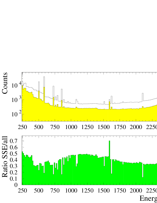
Figure 2: Expected result of PSA from the simulation of the ²²⁸Th- calibration spectrum. Upper panel: Simulated spectra of all events (open histogram) and SSE events only (shaded histogram). Lower panel: Simulated ratio of SSE’s in the spectrum as a function of energy. In the energy region of 0$\nu\beta\beta$-decay a reduction by a factor of $\sim$2.8 can be expected.

4 Digital Pulsform Analysis with Neural Networks

In order to perform PSA a sufficiently large library of known reference pulses has to be collected for the training process. A reliable source of the two different kinds of pulses is needed for this reason. It is well known that high energetic (E $>$ 500 keV) total absorption peaks consist mainly of Compton scattered events (see. [9]). The amount of MSE’s in these peaks in general is not less than 80%. In contrast to this, Double-Escape peaks (pair production followed by the annihilation of the e⁺ and the escape of both 511 keV $\gamma$’s) consist of SSE’s only, since the detected particle in this case is a single electron with energy

$$E_{DE}=(E_{0}-2\times 511~{}keV),$$ (7)

whose dissipation length again is smaller than the time resolution of the detector allows to resolve. Only the Compton background from higher energetic peaks in this area contributes to a contamination of MSE’s in the peak region of the Double-Escape line. Using a ²²⁸Th-calibration source, the Double-Escape line of the total absorption peak at 2614.53 keV with an energy of E_DE=1592.5 keV can be used for the SSE sample. To avoid systematic effects in the training process, a total absorption peak with a similar energy should be used for the MSE sample. The peak at 1621 keV from the ²²⁸Th-daughter nuclide ²¹²Bi seemed appropriate for this purpose.

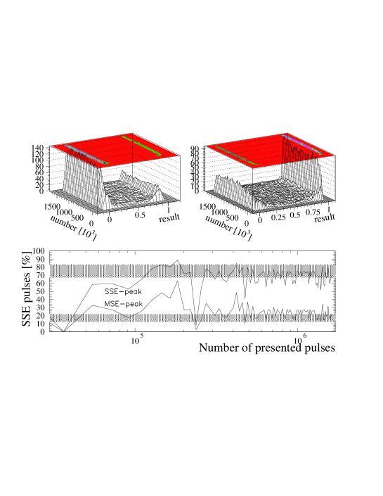
Figure 3: Evolution of the network during the training process. The result of the network after feeding it training pulses was monitored during the training process. Upper panel: The Events with the results from the network are shown as a function of the number of presented pulses. Left: Result from SSE-sample (1592 keV) Right: Same for MSE-sample (1621 keV). Lower panel: Fraction of identified SSE’s in a given sample of reference pulses as a function of number of presented pulses. The shaded areas correspond to the expectation (one sigma band) obtained from the simulation.

5 Simulation of PSA

To test the efficiency and the reliability of the new method we performed simulations of calibration measurements of the Heidelberg-Moscow-Experiment. It is especially important to check for a possible energy dependence of the method since the energy of the training pulses ($\sim$ 1.6 MeV) does not coincide with the energy region of the expected 0$\nu\beta\beta$-decay signature (2038.5 keV). For this purpose we used the GEANT3.21 Monte-Carlo code [10] extended for low energetic decays. The geometry of the experiment and the library of low energetic decays was programmed and successfully tested in earlier works [11, 12]. The code was further extended to distinguish between multiple and single interaction events [13]. In Fig. 2 the simulated spectra of a calibration measurement with a ²²⁸Th source with the whole setup of the Heidelberg-Moscow-Experiment and the resulting expected ratio of SSE’s in the spectrum are shown. In the energy region of the 0$\nu\beta\beta$-decay  between 2000 keV and 2080 keV a reduction factor of $\sim$2.8 is expected through the use of PSA.

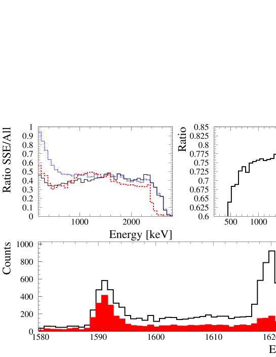
Figure 4: Upper Panel left: Fraction of SSE’s in the spectrum obtained using Neural Network (solid line), applying the one-parameter cut (densely dashed line) and the expectation from the simulation (losely dashed line). Upper panel right: Fraction of pulses identified identically by Neural Network and one-parameter cut. Lower panel: Measured spectrum in the energy region of the reference pulses (data independent of the training sample). The filled histogram corresponds to the identified SSE pulses. The open histogram shows the spectrum of all events.

6 Network results

We recorded $\sim$ 20.000 events of each kind (1592 keV Double-Escape line and 1621 keV total absorption peak) with every detector of the Heidelberg-Moscow-Experiment in the Gran Sasso Underground laboratory. After arranging these pulses in a library, they were used to train the networks. Since the Pulseshapes are dependent on detector parameters like size and form of the crystal, an own network had to be configured for every detector used in the PSA.

The Neural Networks used in this analysis consisted out of three layers: An input layer out of 180 neurons, a hidden layer with 90 neurons and an output layer with a single neuron.

To check the network also during the training process, we monitored the evolution of the network with time, i.e. with the number of presented pulses. This is shown in Fig. 3 for one of the enriched detectors: In the upper panel the output of the Network for the training peaks of the MSE and SSE lines are depicted separately as a function of time. It is evident that the network stabilizes after $\sim$ 400.000 presented pulses (i.e. each pulse has been passed to the network $\sim$ 10 times) and is able to distinguish between the two types of events. The fact that the network is able to identify the contamination of wrong pulses (from the admixture of SSE’s to the MSE sample and of MSE’s to the SSE sample) in the separate libraries gives us further confidence in the power of the method. This is shown in the lower panel. Here the fraction of identified SSE Pulses within the two samples of the training pulses is drawn as a function of presented pulses. The shaded areas give the one sigma region for the expectation obtained from simulations (see section 5). Note that the fraction of ’wrong pulses’ in the libraries is not an input parameter to the training process. This behaviour is obtained solely by the presentation of the reference pulses, i.e. the Neural Network itself recognizes the contamination without previous knowledge.

From Fig. 3 it is obvious that further training of the network is meaningless after a certain limit, the obtained separation into MSE and SSE is not stabilizing further after $\sim$ 400.000 presented pulses. The separation is fluctuating around its mean value from here on. This is probably due to the fact that a non negligible amount of wrong pulses is contained in the training samples. In principle it would be possible to remove a large amount of this contamination since the network identifies wrong pulses within the samples itself. However it seemed too dangerous to use this method for further training since this could give rise to sytematic effects.

Once the training process is finished, it is important to check the obtained results with independent data not used in the training process. We saved one thousand events of each kind for every detector to do this test. The result is seen in Fig. 5. As is evident, also for the independent data the separation works very well (for a quantitative analysis see section 7).

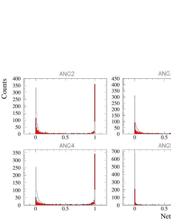
Figure 5: Result of the trained networks tested on independent data, i.e. on pulses which were not used for the training process. The blank histograms correspond to results of events from the SSE-library (expected result: 0), the filled histograms to events from the MSE-library (expected result: 1). Note that the network identifies the contamination with wrong pulses in the refernce libraries correctly.

In Fig. 5 it is visible that for a non-negligible fraction of the pulses an output $y_{o}$ between 0.1 and 0.9 is returned from the network, i.e. the pulses are not properly attributed to a definite type. The fraction of these pulses is $\sim$ 20% for all the detectors. This quantity can be identified as the efficiency of the separation. However, since we have further information from the simulation, we use this fact first to adjust the outcome of the networks to the expectations from the simulation. We define a cut value $\zeta$ so that all pulses with $y_{o}<\zeta$ are identified as SSE. To adjust the network to the expected result we vary $\zeta$ and perform a least square fit for the simulated and measured SSE ratios over the whole energy range above 500 keV. Having found the best fit, this cut is applied to the network result and thus the SSE-spectra are obtained. Note that separation between the two type of events has been obtained this way in Fig. 3. The result with this cut value $\zeta$ is then used to calculate the efficiencies $e_{s}$ and $e_{m}$ of the correct identification of SSE pulses and MSE pulses (see section 7).

In the lower panel of Fig. 4 the obtained result for the energy-region around the reference pulses is shown. Most events in the Double-Escape-line are recognized as SSE’s. Only a small fraction from the background contributes to a contamination of MSE’s. Also the 1621 keV peak is recognized correctly to consist mainly of MSE’s.

7 Comparison with the simulation and the old parameter cut

To compare the results of simulation and measurement directly, the measured and expected ratios of SSE’s in the spectrum as a function of energy are shown in Fig. 4 together with the result from the old one-parameter method. It is evident that the result from the neural netwok is satisfactory over the whole energy range above $\sim$ 500 keV. Only below $\sim$1000 keV there is a noticable difference between the neural network method and the old method. Here the old cut yields too many SSE pulses. Note that especially in the energy region interesting for 0$\nu\beta\beta$-decay  (2000 keV-2080 keV) the agreement of the two techniques is very good.

Detector	Ratio measured	Ratio simulated	Ratio measured	Ratio simulated
	Double-Escape Peak 1592 keV		1621 keV Peak
ANG2	70.9$\pm$2.7	71.7$\pm$7.7	28.3$\pm$1.7	18.0$\pm$4.8
ANG3	72.4$\pm$2.7	75.1$\pm$7.8	29.2$\pm$1.7	17.5$\pm$4.7
ANG4	72.2$\pm$2.7	74.8$\pm$7.3	29.9$\pm$1.7	18.5$\pm$3.4
ANG5	76.0$\pm$2.8	76.4$\pm$8.5	28.7$\pm$1.7	17.4$\pm$4.5

Table 1: Fraction of identified SSE events in the peak areas of the Double-Escape 1592 keV line and the total absorption 1621 keV peak and their expectations from the simulation.

In Tab. 1 the fraction of identified SSE’s in the Double-Escape peak is listed for the four detectors together with the expected results from the simulation. As evident, the measured results are in good agreement with the expectation for the Double-Escape peak. The situation for the measured SSE fraction in the 1621 keV peak is slightly different. Since the efficiency $e_{m}$ for correct identification of MSE’s is not 100%, the actual measured SSE fraction within this peak is somewhat higher than the expected fraction from the simulation. Once the real fraction of SSE’s in a certain energy region is known through e.g. a simulation, it is easy to calculate the efficiencies of the recognition:

$$e_{s}=\frac{1}{\gamma_{s}}+\left(1-\left(\frac{a}{s}\right)_{SSE}\right)\frac{\frac{1}{\gamma_{s}}-\frac{1}{\gamma_{m}}}{\left(\frac{a}{s}\right)_{SSE}-\left(\frac{a}{s}\right)_{MSE}}$$ (8)

and

$$e_{m}=1-\frac{\frac{1}{\gamma_{s}}-\frac{1}{\gamma_{m}}}{\left(\frac{a}{s}\right)_{SSE}-\left(\frac{a}{s}\right)_{MSE}}$$ (9)

where $\gamma_{m}=s_{MSE}$/S_MSE is the ratio of real SSE events in the 1621 keV peak to events identified as SSE’s by the network within the peak, $\gamma_{s}=s_{SSE}$/S_SSE is the according fraction for the Double-Escape-peak and $(\frac{a}{s})_{MSE}$ and $(\frac{a}{s})_{SSE}$ are the simulated ratios of all events to SSE events in the given energy region. The total efficiency $e_{tot}$ of the method is then given by the square root of the product of the two single efficiencies.

The obtained efficiencies for the four networks in the Heidelberg-Moscow-Experiment  are listed in Tab. 2.

Detector	$e_{s}$	$e_{m}$	$e_{tot}$
ANG2	0.93$\pm$0.27	0.86$\pm$0.25	0.90$\pm$0.38
ANG3	0.91$\pm$0.26	0.84$\pm$0.24	0.87$\pm$0.37
ANG4	0.91$\pm$0.19	0.84$\pm$0.17	0.87$\pm$0.27
ANG5	0.95$\pm$0.27	0.85$\pm$0.24	0.90$\pm$0.38

Table 2: Efficiencies for correct SSE and MSE identification for the detectors of the Heidelberg-Moscow-Experiment by neural network.

Obviously an efficient separation of MSE and SSE pulses can be accomplished with Neural Networks. In principle it is possible to correct the result of the network through the known efficiencies with the relation

$$s=\frac{S-(1-e_{m})A}{(e_{s}+e_{m}-1)}.$$ (10)

Here S is the number of SSE’s identified by the network, A is the total number of events and $s$ is the real amount of SSE in the sample A. In our case the correction yields a smaller SSE rate $s$ then actually obtained with the neural networks S, since the number of MSE’s identified as SSE’s is larger than the number of SSE’s identified as MSE’s.

$$(1-e_{m})(A-s)>(1-e_{s})s.$$ (11)

However, we decided not to make use of this correction. Since the obtained efficiencies are high, the correction would be only of the order of 30% in the case of a large ratio $\frac{a}{s}$, as realized for total absorption peaks. The correction would be of the order of $\sim$10% for the expected ratio in the 0$\nu\beta\beta$-decay energy range. The fact that we do not apply the correction makes the use of the new technique a conservative method.

From the ratio of identified SSE pulses in the energy region between 2000 keV and 2080 keV it is expected that the background in the calibration spectrum can be further reduced by a factor of 2.67$\pm$0.05 which is in good agreement with the results obtained from the simulation which yields a reduction factor of 2.78$\pm$0.01 and the one parameter-cut, which gives a reduction by a factor of 2.53$\pm$0.05 The slightly smaller value in the measurement is the effect of the efficiencies for the recognition. We expect a similar reduction for the Heidelberg-Moscow-Experiment.

To finally check the compatibility of the two methods, in the right diagram of Fig. 4 we show the fraction of pulses from the library which were attributed the same type from both methods as a function of energy. With the efficiencies given above and the efficiencies of the old method we expect a fraction of $\sim$ 70 % to be identified equaly. Indeed $\sim$75% of the events are classified equally.

8 Conclusion

We developed a new method to distinguish between multiple scattered and single interaction events in HPGe-detectors on the basis of Neural Networks. We showed that this technique is capable of distinguishing between the two types of events with a very high efficiency. The comparison with a simulation performed for this purpose confirms these results.

9 Aknowledgement

B. M. would like to thank Ch. Gund for help with the extension of the GEANT3.21 code. B. M. is supported by the Graduiertenkolleg of the University of Heidelberg.

References

- [1] Y. Fukuda et al., The SuperKamiokande Collaboration, Phys. Rev. Lett. 81(1998)1562 and Preprint hep-ex/9807003
- [2] H.V. Klapdor-Kleingrothaus, Int. J. Mod. Phys A 13(1998)3953 and H.V. Klapdor-Kleingrothaus in Lepton and Baryon Number Violation, Proceedings of the First International Symposium on Lepton and Baryon Number Violation, Trento, 20-25 April 1998, editors H.V. Klapdor-Kleingrothaus and I.V. Krivosheina, IoP Bristol, 1999, page 251
- [3] J. Valle in Proccedings of New Trends in Neutrino Physics, May 1998, Castle Ringberg, Tegernsee, Germany and Preprint, hep-ph/9809234
- [4] Heidelberg Moscow Collaboration, L. Baudis et al. Phys. Rev. Lett. 83(1999)41 and Preprint hep-ex/9902014
- [5] J. Hellmig, PhD thesis, Univerity of Heidelberg, 1996
- [6] Heidelberg Moscow Collaboration, L. Baudis et al., Physics Letters B 407(1997)219-224
- [7] K. Hornik, M. Stinchcombe, H. White, Neural Networks, 1989, 2(5),359-366, G. Cybenko, Mathematics of Control, Signals and Systems, 1989, 2(4), 303-314
- [8] B. Kröse and P. van der Smagt, University of Amsterdam, An Introduction to Neural Networks, 1996
- [9] J. Roth et al., IEEE Trans. Nucl. Sci., NS-31(1984)367
- [10] GEANT3.21, Detector description and simulation tool, CERN long-writeup, 1993
- [11] B. Maier, PhD thesis, University of Heidelberg, 1995
- [12] A. Dietz, diploma thesis, University of Heidelberg, 1999, unpublished
- [13] Ch. Gund, private communication