CERN–EP/99–139 xx Università ‘La Sapienza’ and Sezione INFN di Roma 1, Rome, Italy, and CERN, Geneva, Switzerland
Email: dagostini@roma1.infn.it
URL: http://www-zeus.roma1.infn.it/^∼agostini

This paper is meant as a contribution to the often debated subject of how to combine data which appear to be in mutual disagreement. As a practical example, the $\epsilon^{\prime}/\epsilon$ determinations have been considered.

(Submitted to Physical Review D)

1 Introduction

Every physicist knows the rule for combining several experimental results:

$$\mu = \frac{\sum_{i}d_{i}/s_{i}^{2}}{\sum_{i}1/s_{i}^{2}}$$ (1)

$$\sigma(\mu) = \left(\sum_{i}1/s_{i}^{2}\right)^{-\frac{1}{2}}\,,$$ (2)

where ‘$\mu$’ refers to the true value and $d_{i}\pm s_{i}$ stands for the individual data point (the use of $s_{i}$, instead of the usual $\sigma_{i}$, for the standard uncertainty reported by the experiments will become clear later; similarly, the meaning of ‘$\mu$’ and of $\sigma(\mu)$ have not been well defined for the moment, as they will be better defined later). The above rule, hereafter called standard combination rule, is based on some hypotheses which are worth recalling: i) all measurements refer to the same quantity; ii) the measurements are independent; iii) the probability distribution of $d_{i}$ around $\mu$ is described by a Gaussian distribution with standard deviation given by $\sigma_{i}=s_{i}$. If one, or several, of these hypotheses are not satisfied, the result of Eqs. (1)–(2) is questionable.

Now we are confronted with the problem that we are never absolutely sure if these hypotheses are true or not. If we were absolutely convinced that the hypotheses were correct, there would be no reason to hesitate to apply Eqs. (1)–(2), no matter how ‘apparently incompatible’ the data points might appear. But we know by experience that unrecognized sources of systematic errors might affect the results, or that the uncertainty associated with the recognized sources might be underestimated (but we also know that, often, this kind of uncertainty is prudently overstated…).

As is always the case in the domain of uncertainty, there is no ‘objective’ method for handling this problem; neither in deciding if the data are in mutual disagreement, nor in arriving at a universal solution for handling those cases which are judged to be troublesome. Only good sense gained by experience can provide some guidance. Therefore, all automatic ‘prescriptions’ should be considered cum grano salis. For example, the usual method for checking the hypothesis that ‘the data are compatible with each other’ is to make a $\chi^{2}$ test. The hypothesis is accepted if, generally speaking, the $\chi^{2}$ does not differ too much from the expected value. As a strict rule, the $\chi^{2}$ test is not really logically grounded (see e.g. Section 1.8 of Ref. [1]) although it does ‘often work’, due to implicit hypotheses which are external to the standard $\chi^{2}$ test scheme (see Section 8.7 of Ref. [1]), but which lead to mistaken conclusions when the unstated hypotheses are not reasonable (see e.g. Section 1.9 of Ref. [1]). Therefore, I shall not attempt here to quantify the degree of suspicion. I shall assume a situation in which experienced physicists, faced with a set of results, tend to be uneasy about the mutual consistency of the picture that those data offer.

As an example, let us consider the results of Table 1,

Table 1: Published results on Re($\epsilon^{\prime}/\epsilon$) (values in units of $10^{-4}$). Data points indicated by $\surd$ have been used for quantitative evaluations. Owing to correlations between the 1988 and 1993 uncertainties of NA31, only the combined value published in 1993 is used protect[6].

Experiment		Central value	$\pm\sigma_{\mbox{\it stat}}\pm\sigma_{\mbox{\it syst}}$	$\sigma_{\mbox{\it tot}}$
$\surd$	E731 (1988) [2]	32	$\pm 28\pm 12$	30
	NA31 (1988)[3]	33	$\pm 6.6\pm 8.3$	11
$\surd$	E731 (1993)[4]	7.4	$\pm 5.2\pm 2.9$	5.9
	NA31 (1993)[5]	20	$\pm 4.3\pm 5.0$	7
$\surd$	NA31 (1988+1993)[5, 6]	23.0	$\pm 4\pm 5$	6.5
$\surd$	KTeV (1999)[7]	28.0	$\pm 3.0\pm 2.8$	4.1
$\surd$	NA48 (1999)[8]	18.5	$\pm 4.5\pm 5.8$	7.3

which are also reported in a graphical form in Fig. 1. Figure 2 shows also the combined result obtained using Eqs. (1)–(2), as well as some combinations of subsamples of the results.

Figure 1: Results on Re($\epsilon^{\prime}/\epsilon$) obtained at CERN (solid line) and Fermilab (dashed line), where $e={\rm Re}(\epsilon^{\prime}/\epsilon)\times 10^{4}$.

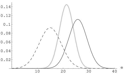
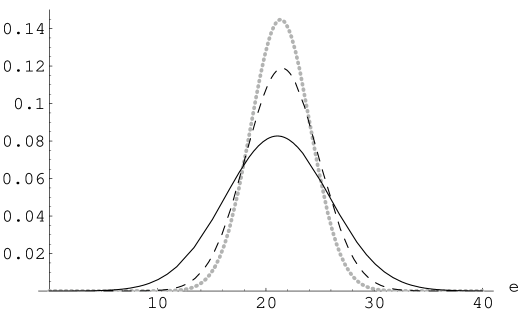
Figure 2: Some combinations of the experimental results obtained using the standard combination rule of Eqs. (1)–(2). Upper plot: old results (dashed line), 1999 results (solid line), overall combination (dotted grey line). Lower plot: CERN experiments (solid line), Fermilab experiments (dashed), overall combination (dotted grey line).

These results have not been chosen as the best example of disagreeing data, but because of the physics interest, and also because the situation is at the edge of where one starts worrying. The impression of uneasiness is not only because the mutual agreement among the experimental results is not at the level one would have wished, but also because the value of Re($\epsilon^{\prime}/\epsilon$) around which the experimental results cluster is somewhat far from the theoretical evaluations (see e.g. Refs. [9, 10, 11, 12, 13] and references therein). Now, it is clear that experimentalists should not be biased towards theoretical expectations, and the history of physics teaches us about wrong results published to please theory. But we are also aware of unexpected results (either claims of new physics, or simply a quantitative disagreement with respect to the global scenario offered by other results within the framework of the Standard Model) which finally turn out to be false alarms. In conclusion, given the present picture of theory versus experiments about $\epsilon^{\prime}/\epsilon$, there is plenty of room for doubt: Doubt about theory, about individual experiments, and about experiments as a whole.

In this situation, drawing conclusions based on a blind application of Eqs. (1)–(2) seems a bit naïve. For example, a straightforward conclusion of the standard combination rule leads to a probability that Re($\epsilon^{\prime}/\epsilon$) is smaller than zero of the order of $0.5~{}\times~{}10^{-14}$, and I don’t think that experienced physicists would share without hesitation beliefs of this order of magnitude.

This paper deals with modelling the beliefs of an experienced sceptical physicist confronted with results of this kind, continuing on from a recent work of Dose and von der Linden on outliers [14].

2 Hypotheses behind the simple combination rule

Equation (1) has been written, on purpose, in a way that might be misleading, although this is the way in which it often appears. In fact, taken literally, it says that $\mu$ is equal to the right-hand side of Eq. (1). Instead, as is well understood, this is just the value around which our beliefs are centred, usually referred to as the estimator. Given a Gaussian model, the estimator given by Eq. (1) corresponds to the value which we believe mostly (mode), and also to the barycentre of the probability distribution of $\mu$ (expected value) and to the value which defines two semi-open intervals in each of which we believe $\mu$ to lie with equal probability (median).

In order to obtain a combination rule different from Eqs. (1)–(2), it is important to remember where these formulae come from. Although this rule is usually taught in the framework of maximum likelihood, the most general way to get it is by using Bayesian inference, as we shall show now.

The simplest way to write Bayes’ theorem for continuous variables is:

$$f(\mu\,|\,\underline{d})\propto f(\underline{d}\,|\,\mu)\cdot f_{\circ}(\mu)\,,$$ (3)

where the set of data points $\{d_{1},d_{2},\ldots,d_{n}\}$ is indicated by $\underline{d}$; the function $f(\mu\,|\,\underline{d})$ is the final probability density function (p.d.f.) of $\mu$ in the light of the experimental results and of all other prior knowledge about measurement and measurand; $f(\underline{d}\,|\,\mu)$ represents the likelihood of observing the data set $\underline{d}$ under the hypothesis that the true value is exactly $\mu$; $f_{\circ}(\mu)$ is the prior p.d.f. of $\mu$. The proportionality factor is obtained by the normalization condition $\int\!f(\mu\,|\,\underline{d})\,\mbox{d}\mu=1$. The assumption that each of the observed values is normally distributed around $\mu$ with standard deviation $\sigma_{i}$ and that the measurements are independent leads to

$$f(\underline{d}\,|\,\mu)=\prod_{i}\frac{1}{\sqrt{2\,\pi}\,\sigma_{i}}\,\exp\left[-\frac{(d_{i}-\mu)^{2}}{2\,\sigma_{i}^{2}}\right]\,.$$ (4)

If the experimental resolution described by the likelihood is sufficiently high and $\mu$ is a quantity which can assume, in principle, values in a large interval (virtually any real values), a uniform prior distribution, i.e. $f_{\circ}(\mu)=k$, is a very reasonable assumption. In fact, any other mathematical function which models the vagueness of the prior knowledge (with respect to what the measurement is supposed to yield) acts in practice as a constant in the region of $\mu$ where the likelihood varies rapidly. Putting all the ingredients together and renormalizing the final p.d.f. we get

$$f(\mu\,|\,\underline{d},\mbox{indep. Gaussians},\underline{\sigma},f_{\circ}(\mu)=k)=\frac{1}{\sqrt{2\,\pi}\,\sigma(\mu)}\,\exp\left[-\frac{(\mu-\mbox{E}[\mu])^{2}}{2\,\sigma^{2}(\mu)}\right]\,,$$ (5)

where

$$\mbox{E}[\mu] = \frac{\sum_{i}d_{i}/s_{i}^{2}}{\sum_{i}1/s_{i}^{2}}$$ (6)

$$\sigma(\mu) = \left(\sum_{i}1/s_{i}^{2}\right)^{-\frac{1}{2}}\,,$$ (7)

obtained assuming that the $\sigma_{i}$ of Eq. (4) are exactly equal to the quoted stated uncertainties $s_{i}$. In Eq. (5) all conditions have been explicitly stated. This derivation shows that there is indeed a fourth important implicit assumption in order to arrive at Eqs. (1)–(2), namely a uniform prior on $\mu$. This is why the maximum belief coincides with the maximum of the likelihood, and why the best estimate of $\mu$ is the same as is obtainable from the maximum likelihood principle. Nevertheless, the route followed here is more general and more intuitive, as discussed extensively in Ref. [1]. In particular, one can speak consistently about probability of true values, a concept close to the natural reasoning of physicists [17].

3 Probabilistic modelling of scepticism

Once we have understood what is behind the simple combination rule, it is possible to change one of the hypotheses entering Eq. (5). Obviously, the problem has no unique solution. This depends to a great extent on the status of knowledge about the experiments which provided the results. For example, if one has formed a personal idea concerning the degree of reliability of the different experimental teams, one can attribute different weights to different results, or even disregard results considered unreliable or obsolete (for example their corrections for systematic effects could depend on theoretical inputs which are now considered to be obsolete). Wishing to arrive at a solution which, with all the imaginable limitations a general solution may have, is applicable to many situations without an inside, detailed knowledge of each individual experiment, we have to make some choices. First, we decide that our sceptic is democratic, i.e. ‘he’ has no a priori preference for a particular experiment. Second, the easiest way of modelling his scepticism, keeping the mathematics simple, is to consider the likelihood still Gaussian, but with a standard deviation which might differ from that quoted by the experimentalists by a factor $r_{i}$ which is not exactly known:

$$r_{i}=\frac{\sigma_{i}}{s_{i}}~{}.$$ (8)

The uncertainty about $r_{i}$ can be described by a p.d.f. $f(r_{i})$. This uncertainty changes each factor appearing in the likelihood (4), as can be evaluated by the probability rules:

$$f(d_{i}\,|\,\mu)=\int\!f(d_{i}\,|\,\mu,r_{i})\cdot f(r_{i})\,\mbox{d}r_{i}\,,$$ (9)

with

$$f(d_{i}\,|\,\mu,r_{i},s_{i})=\frac{1}{\sqrt{2\,\pi}\,r_{i}\,s_{i}}\,\exp\left[-\frac{(d_{i}-\mu)^{2}}{2\,r_{i}^{2}\,s_{i}^{2}}\right]\,.$$ (10)

If one believes that all $r_{i}$ are exactly one, i.e. $f(r_{i})=\delta(r_{i}-1)\ \forall\,i$, the standard combination rule is recovered. Because of our basic assumption of democracy, the mathematical expression of the p.d.f. of $r_{i}$ will not depend on $i$, therefore we shall talk hereafter, generically, about $r$ and $f(r)$.

A solution to the problem of finding a parametrization of $f(r)$ such that this p.d.f. is acceptable to experienced physicists, even though the integral (9) still has a closed form, has been proposed by Dose and von der Linden [14]; an improved version of it will be used in this paper [18]. Following Ref. [14], we choose initially the variable $\omega=1/r^{2}=s_{i}^{2}/\sigma_{i}^{2}$, and consider it to be described by a gamma distribution:

$$f(\omega)=\frac{\lambda^{\delta}\,\omega^{\delta-1}\,e^{-\lambda\,\omega}}{\Gamma(\delta)}\,,$$ (11)

where $\lambda$ and $\delta$ are the so-called scale and shape parameters, respectively. As a function of these two parameters, expected value and variance of $\omega$ are $\mbox{E}[\omega]=\delta/\lambda$ and $\mbox{Var}(\omega)=\delta/\lambda^{2}$. Using probability calculus we get the p.d.f of $r$:

$$f(r\,|\,\lambda,\delta)=\frac{2\,\lambda^{\delta}\,r^{-(2\,\delta+1)}\,e^{-\lambda/r^{2}}}{\Gamma(\delta)}\,,$$ (12)

where the parameters have been written explicitly as conditionands for the probability distribution. Expected value and variance of $r$ are:

$$\mbox{E}[r] = \frac{\sqrt{\lambda}\,\Gamma(\delta-1/2)}{\Gamma(\delta)}$$ (13)

$$\mbox{Var}(r) = \frac{\lambda}{\delta-1}-\frac{\lambda\,\Gamma^{2}(\delta-1/2)}{\Gamma^{2}(\delta)}\,,$$ (14)

existing simultaneously if $\lambda>0$ and $\delta>1$.

The individual likelihood, integrated over the possible values of $r$, is obtained by inserting Eqs. (10) and (12) in Eq. (9):

$$f(d_{i}\,|\,\mu,s_{i})=\frac{\lambda^{\delta}}{\sqrt{2\,\pi}s_{i}}\,\frac{\Gamma(\delta+1/2)}{\Gamma(\delta)}\,\left(\lambda+\frac{(d_{i}-\mu)^{2}}{2\,s_{i}^{2}}\right)^{-(\delta+1/2)}\,.$$ (15)

Using a uniform prior distribution for $\mu$, and remembering that we are dealing with independent results, we have finally:

$$f(\mu\,|\,\underline{d},\underline{s})\propto f(\underline{d}\,|\,\underline{s},\mu)\propto\prod_{i}\left(\lambda+\frac{(d_{i}-\mu)^{2}}{2\,s_{i}^{2}}\right)^{-(\delta+1/2)}\,,$$ (16)

where $\underline{s}=\{s_{1},s_{2},\ldots,s_{n}\}$. The normalization factor can be determined numerically. Equation (16) should be written, more properly, as $f(\mu\,|\,\underline{d},\underline{s},\lambda,\delta)$, to remind us that the solution depends on the choice of $\lambda$ and $\delta$, and teaches us how to get a solution which takes into account all reasonable choices of the parameters:

$$f(\mu\,|\,\underline{d},\underline{s})=\int\!f(\mu\,|\,\underline{d},\underline{s},\lambda,\delta)\cdot f(\lambda,\delta)\,\mbox{d}\lambda\mbox{d}\delta\,,$$ (17)

where $f(\lambda,\delta)$ quantifies the confidence on each possible pair of parameters.

A natural constraint on the values of the parameters comes from the request $\mbox{E}[r]=1$, modelling the assumption that the $\sigma$’s agree, on average, with the stated

uncertainties. The standard deviation of the distribution gives another constraint. Conservative considerations suggest $\sigma(r)/\mbox{E}[r]\approx{\cal O}(1)$. The condition $\mbox{E}[r]=\sigma(r)$ = 1 is obtained for $\lambda\approx 0.6$ and $\delta\approx 1.3$. The resulting p.d.f. of $r$ is shown as the continuous line of Fig. 3.

Figure 3: Distribution of the rescaling factor $r=\sigma_{\mbox{true}}/\sigma_{\mbox{est}}$ using the parametrizations of Eq. (12) for several values of the set of parameters $(\lambda,\delta)$; the solid line corresponds to what will be taken as the reference distribution in this paper, yielding $\mbox{E}[r]=\sigma(r)=1$, and it is obtained for $\lambda\approx 0.6$ and $\delta\approx 1.3$. Dotted and dashed lines show the p.d.f. of $r$ yielding $\sigma(r)=0.5$ and 1.5, respectively.

One can see that the parametrization of $f(r)$ corresponds qualitatively to intuition: the barycentre of the distribution is 1; values below $r\approx 1/2$ are considered practically impossible; on the other hand, very large values of $r$ are conceivable, although with very small probability, indicating that large overlooked systematic errors might occur. Anyway, we feel that, besides general arguments and considerations about the shape of $f(r)$ (to which we are not used), what matters is how reasonable the results look. Therefore, the method has been tested with simulated data, shown in the left plots of Fig. 4.

Individual results	Eq. (16), $\mathbf{\lambda=0.6}$ and $\mathbf{\delta=1.3}$
	$[\mathbf{\sigma(r)=1}]$

                       $2\,\times$

Figure 4: Examples of sceptical combination of results. The plots on the left-hand side show the individual results (in the upper plot the two results coincide). The plots on the right-hand side show the combined result obtained using Eq. (16) with the constraint $\mbox{E}[r]=\sigma(r)=1$ (continuous lines), compared with the standard combination (dashed lines).

Eq. (16), $\lambda=1.4$ and $\delta=2.1$	Eq. (16), $\lambda=0.4$ and $\delta=1.1$
$[\sigma(r)=0.5]$	$[\sigma(r)=1.5]$

Figure 5: Combination of results obtained by varying the parameters of the sceptical combination.

Figure 6: Sceptical perception of a single measurement having a standard deviation equivalent to the standard combination of the top of Fig. 4. Note how the result differs from the combination of the individual results.

For simplicity, all individual results are taken to have the same standard deviation (note that the upper left plot of Fig. 4 shows the situation of two identical results). The solid curve of the right-hand plots shows the combined result obtained using Eq. (16) with $\lambda=0.6$ and $\delta=1.3$, yielding $\mbox{E}[r]=\sigma(r)=1$. For comparison, the dashed lines show also the result obtained by the standard combination. The method described in this paper, with parameters chosen by general considerations, tends to behave in qualitative agreement with the expected point of view of a sceptical experienced physicist. As soon as the individual results start to disagree, the combined distribution gets broader than the standard combination, and might become multi-modal if the results cluster in several places. However, if the agreement is somehow ‘too good’ (first and last case of Fig. 4) the combined distribution becomes narrower than the standard result.

In order to get a feeling about the sensitivity of the results from the choice of the parameters, two other sets of parameters have been tried, keeping the requirement $\mbox{E}[r]=1$, but varying $\sigma(r)$ by $\pm$50 %: $\sigma(r)$ = 0.5 is obtained for $\lambda\approx$ 1.4 and $\delta\approx$ 2.1; $\sigma(r)=1.5$ is obtained for $\lambda\approx$ 0.4 and $\delta\approx$ 1.1. The resulting p.d.f.’s of $r$ are shown in Fig. 3. The results obtained using these two sets of parameters on the simulated data of Fig. 4 are shown in Fig. 5. We see that, indeed, the choice $\mbox{E}[r]=\sigma(r)=1$ seems to be an optimum, and the $\pm 50\%$ variations of $\sigma(r)$ give results which are at the edge of what one would consider to be acceptable. Therefore, we shall take the parameters providing $\mbox{E}[r]=\sigma(r)=1$ as the reference ones.

Another interesting feature of Eq. (16) is its behaviour for a single experimental result, as shown in Fig. 6. For comparison, we have taken a result having a stated standard deviation equal to $1/\sqrt{2}$ of each of those of Fig. 4. Figure 6 has to be compared with the upper right plots of Fig. 4. The sceptical combination takes much more seriously two independent experiments, each reporting in an uncertainty $\sigma$, than a single experiment performing $\sigma/\sqrt{2}$. On the contrary, the two situations are absolutely equivalent in the standard combination rule. In particular, the tails of the p.d.f. obtained by the sceptical combination vanish more slowly than in the Gaussian case, while the belief in the central value is higher. The result models the qualitative attitude of sceptical physicists, according to whom a single experiment is never enough to establish a value, no matter how precise the result may be, although the true value might have more chance to be within one standard deviation than the probability level calculated from a Gaussian distribution.

4 Application to $\epsilon^{\prime}/\epsilon$

The combination rule based on Eq. (16) has been applied to the results about Re($\epsilon^{\prime}/\epsilon$) shown in Table 1. As discussed above, our reference parameters are $\lambda=0.6$ and $\delta=1.3$, corresponding to $\mbox{E}[r]\approx\sigma(r)\approx 1$. The resulting p.d.f. for $e$ = Re($\epsilon^{\prime}/\epsilon)\times 10^{4}$ is shown as the thick continuous line of Fig. 7, together with the individual results (dotted lines). For comparison, we also give the result obtained using the combination rules commonly applied in particle physics. The grey-dashed line of Fig. 7 is obtained with the standard combination rule [Eqs. (1) and (2)]. The thin continuous line has been evaluated using the Particle Data Group (PDG) ‘prescription’ [19]. According to this rule, the standard deviation (2) is enlarged by a factor given by $\sqrt{\chi^{2}/(N-1)}$, where $\chi^{2}$ is the chi-2 of the data with respect to the average (1) and $N$ is the number of independent results.

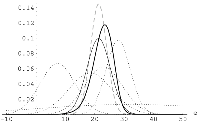
Figure 7: Individual results compared with the standard combination (grey dashed), the PDG-rescaled combination (solid thin) and the sceptical combination as described in this paper (solid thick).

Table 2: Comparison of the different methods of combining the results.

Combination	Mean ($\sigma$)	Median	Mode	99% range	$P[{\rm Re}(\epsilon^{\prime}/\epsilon<0)]$
			$\pm\,34\%$ range
Standard	$21.4\,(2.7)$	21.4	$21.4\pm 2.7$	$[14.3,28.5]$	$5\times 10^{-15}$
PDG rule [19]	$21.4\,(4.0)$	21.4	$21.4\pm 4.0$	$[11.0,31.7]$	$5\times 10^{-8}$
Sceptical	22.7 (3.5)	23.0	$23.5\pm 3.4$	$[11.6,30.5]$	$1.5\times 10^{-6}$

We see that although the PDG rule gives a distribution wider than that obtained by the standard rule, the barycentres of the distributions coincide, thus not taking into account that one of the results is quite far from where the others seem to cluster. Moreover, the p.d.f. is assumed to be Gaussian, independently of the configuration of experimental points. Instead, the sceptical combination takes into account better the configuration of the data points. The peak of the distribution is essentially determined by the three results which appear more consistent with each other. Nevertheless, there is a more pronounced tail for small values of Re($\epsilon^{\prime}/\epsilon$), to take into account that there is indeed a result providing evidence in that region, and that cannot be ignored.

A quantitative comparison of the different methods is given in Table 2, where the most relevant statistical summaries are provided (average, mode, median, standard deviation), together with some probability intervals. It is worth recalling that each of these summaries gives some information about the distribution, but, when the uncertainty of this result has to be finally propagated into other results (together with other uncertainties), it is the average and standard deviation which matter. An interesting comparison is given by the probability that Re($\epsilon^{\prime}/\epsilon$) is negative. The sceptical combination gives the largest value, but still at the level of one part per million, indicating that, even in this conservative analysis, a positive value of the direct CP violation parameter seems ‘practically’ established.

The sensitivity of the result on the parameters of the combination formula can be inferred from Fig. 8, where the results obtained changing $\sigma(r)$ by $\pm 50\%$ are shown. The combined result is quite stable. This is particularly true if one remembers that these extreme values of parameters are quite at the edge of what one would accept as reasonable, as can be seen in Fig. 5. Note that if one would like to combine the results taking also into account the uncertainty about the parameters, one would apply Eq. (17). It is reasonable to think that, since the variations of the p.d.f. from that obtained for the reference value of the parameters are not very large, the p.d.f. obtained as weighted average over all the possibilities will not be much different from the reference one.

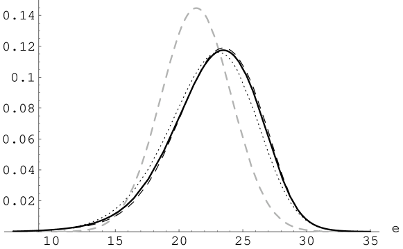
Figure 8: Dependence of the sceptical combination on the choice of the parameters. Continuous, dotted and dashed lines are, in order: $\lambda=0.6$ and $\delta=1.3$ $[\sigma(r)=1)]$; $\lambda=0.4$ and $\delta=1.1$ $[\sigma(r)=0.5)]$; $\lambda=1.4$ and $\delta=2.1$ $[\sigma(r)=0.5)]$. The grey-dashed line gives, for comparison, the result of the standard combination.

Figure 9 and Table 3 give the results subdivided into CERN and Fermilab. In these cases the difference between the standard combination and the sceptical combination becomes larger, and, again, the outcome of the sceptical combination follows qualitatively the intuitive one of experienced physicists. The sceptical combination of the CERN results alone is better than that given by the standard one, thus reproducing formally the

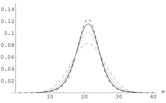
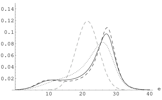
Figure 9: Sceptical combination of CERN and Fermilab results (upper and lower plot, respectively). The continuous line shows the result obtained by Eq. (16) and reference parameters. The dashed and dotted lines are the results obtained by varying the standard deviation of $r=\sigma/s$ by $+50\%$ and $-50\%$, respectively. The grey-dashed line shows the results obtained by the standard combination rule.

Table 3: Comparison of the different methods of combining partial results. The symbol * means that the distribution has less than 34.1% probability on the right side of the mode.

Combination		Mean ($\sigma$)	Median	Mode	99% p. range	$P[\mbox{Re}(\epsilon^{\prime}/\epsilon)<0]$
				$\pm 34\%$ p. range
Stand.	$\left\{\begin{array}[]{l}\mbox{CERN}\\ \mbox{Fermilab}\end{array}\right.$	$\begin{array}[]{l}21.1\,(4.8)\\ 21.4\,(2.7)\end{array}$	$\begin{array}[]{l}21.1\\ 21.4\end{array}$	$\begin{array}[]{l}21.1\pm 4.8\\ 21.4\pm 2.7\end{array}$	$\begin{array}[]{c}\mbox{[8.6, 33.4]}\\ \mbox{[12.9, 30.1]}\end{array}$	$\begin{array}[]{l}6\times 10^{-6}\\ 8\times 10^{-11}\end{array}$
Scept.	$\left\{\begin{array}[]{l}\mbox{CERN}\\ \mbox{Fermilab}\end{array}\right.$	$\begin{array}[]{l}21.0\,(3.9)\\ 23.0\,(7.1)\end{array}$	$\begin{array}[]{l}21.0\\ 25.2\end{array}$	$\begin{array}[]{l}21.1\pm 3.6\\ 27.1^{+\,*}_{-4.9}\end{array}$	$\begin{array}[]{c}\mbox{[9.2, 32.5]}\\ \mbox{[2.7, 36.2]}\end{array}$	$\begin{array}[]{l}2.5\times 10^{-4}\\ 1.5\times 10^{-3}\end{array}$

instinctive suspicion that the uncertainties could have been overestimated. For the Fermilab ones the situation is reversed. In any case, both partial combinations tend to establish strongly the picture of a positive and sizeable Re($\epsilon^{\prime}/\epsilon$) value. Finally, note that the $\pm 50$% variations in $\sigma(r)$ produce in the partial combinations a larger effect (although not relevant for the conclusions) than in the overall combination. This is due to the fact that the variations produce opposite effects on the two subsets of data in the region of Re($\epsilon^{\prime}/\epsilon$) around $20\times 10^{-4}$.

5 Posterior evaluation of $\sigma_{i}$

An interesting by-product of the method illustrated above is the posterior evaluation of the various $\sigma_{i}$, or, equivalently, of the various $r_{i}$. Again, we can make use of Bayes’ theorem, obtaining

$$f(\underline{r}\,|\,\underline{d},\underline{s},\mu)=\frac{f(\underline{d}\,|\,\underline{r},\underline{s},\mu)\cdot f_{\circ}(\underline{r}\,|\,\underline{s},\mu)}{\int\!f(\underline{d}\,|\,\underline{r},\underline{s},\mu)\cdot f_{\circ}(\underline{r}\,|\,\underline{s},\mu)\,\mbox{d}\underline{r}}~{},$$ (18)

where $\underline{r}=\{r_{1},r_{2},\ldots,r_{n}\}$. Since the initial status of knowledge is such that values of $r_{i}$ are independent of each other, and they are independent of $\mu$ and $\underline{s}$, we obtain

$$f_{\circ}(\underline{r}\,|\,\underline{s},\mu)=f_{\circ}(\underline{r})=\prod_{i}f_{\circ}(r_{i})\equiv\prod_{i}f(r_{i}\,|\,\lambda,\delta)=\prod_{i}\frac{2\,\lambda^{\delta}\,r_{i}^{-(2\,\delta+1)}\,e^{-\lambda/r_{i}^{2}}}{\Gamma(\delta)}~{},$$ (19)

having used Eq. (12). As a shorthand for Eq. (19), we shall write in the following simply $f_{\circ}(\underline{r})=\prod_{i}f_{\circ}(r_{i})$.

Since the experimental results are also considered independent, we can rewrite Eq. (18) as

$$f(\underline{r}\,|\,\underline{d},\underline{s},\mu) = \frac{\prod_{i}f(d_{i}\,|\,r_{i},s_{i},\mu)\cdot f_{\circ}(r_{i})}{\int\!\prod_{i}f(d_{i}\,|\,r_{i},s_{i},\mu)\cdot f_{\circ}(r_{i})\,\mbox{d}\underline{r}}$$ (20)

$$= \frac{\prod_{i}f(d_{i}\,|\,r_{i},s_{i},\mu)\cdot f_{\circ}(r_{i})}{\prod_{i}\int\!f(d_{i}\,|\,r_{i},s_{i},\mu)\cdot f_{\circ}(r_{i})\,\mbox{d}r_{i}}\,~{}.$$

The marginal distribution of each $r_{i}$, still conditioned by $\mu$ (and, obviously, by the experimental values), is obtained by integrating $f(\underline{r}\,|\,\underline{d},\underline{s},\mu)$ over all $r_{j}$, with $j\neq i$. As a result, we obtain

$$f(r_{i}\,|\,\underline{d},\underline{s},\mu) = \frac{f(d_{i}\,|\,r_{i},s_{i},\mu)\cdot f_{\circ}(r_{i})}{\int\!f(d_{i}\,|\,r_{i},s_{i},\mu)\cdot f_{\circ}(r_{i})\,\mbox{d}r_{i}}\,~{}.$$ (21)

Making use of Eqs. (10), (12) and (15) we get:

$$f(r_{i}\,|\,\underline{d},\underline{s},\mu) = \frac{\frac{1}{\sqrt{2\,\pi}\,r_{i}\,s_{i}}\,\exp\left[-\frac{(d_{i}-\mu)^{2}}{2\,r_{i}^{2}\,s_{i}^{2}}\right]\cdot\frac{2\,\lambda^{\delta}\,r_{i}^{-(2\,\delta+1)}\,e^{-\lambda/r_{i}^{2}}}{\Gamma(\delta)}}{\frac{\lambda^{\delta}}{\sqrt{2\,\pi}s_{i}}\,\frac{\Gamma(\delta+1/2)}{\Gamma(\delta)}\,\left(\lambda+\frac{(d_{i}-\mu)^{2}}{2\,s_{i}^{2}}\right)^{-(\delta+1/2)}}\,.$$ (22)

The final result is obtained by eliminating, in the usual way, the condition $\mu$, i.e.

$$f(r_{i}\,|\,\underline{d},\underline{s})=\int\!f(r_{i}\,|\,\underline{d},\underline{s},\mu)\cdot f(\mu\,|\,\underline{d},\underline{s})\,\mbox{d}\mu\,~{}.$$ (23)

Making use of Eq. (16), and neglecting in Eq. (22) all factors not depending on $r_{i}$ and $\mu$, we get the unnormalized result

$$f(r_{i}\,|\,\underline{d},\underline{s})\propto r_{i}^{-(2\,\delta+2)}\,e^{-\lambda/r_{i}^{2}}\int\!\exp\left[-\frac{(d_{i}-\mu)^{2}}{2\,r_{i}^{2}\,s_{i}^{2}}\right]\,\prod_{j\neq i}\left(\lambda+\frac{(d_{j}-\mu)^{2}}{2\,s_{j}^{2}}\right)^{-(\delta+1/2)}\,\mbox{d}\mu\,~{}.$$ (24)

This formula is clearly valid for $n\geq 2$. If this is not the case, the product over $j\neq i$ is replaced by unity, and the integral is proportional to $r_{i}$. Equation (24) becomes then $f(r_{1}\,|\,d_{1},s_{1})\propto r_{1}^{-(2\,\delta+1)}\,e^{-\lambda/r_{1}^{2}}$, i.e. we have recovered the initial distribution (12). In fact, if we have only one data point, there is no reason to change our beliefs about $r$. Only the comparison with other results can induce us to change our opinion.

Once we have got $f(r_{i}\,|\,\underline{d},\underline{s})$ we can give posterior estimates of $r_{i}$ in terms of average and standard deviations, and they can be compared with the prior assumption $\mbox{E}[r]=\sigma(r)=1$, to understand which uncertainties have been implicitly rescaled by the sceptical combination. Convenient formulae to evaluate numerically first and second moments of the posterior distribution of $r_{i}$ are given by

$$\mbox{E}[r_{i}] = \frac{\Gamma(\delta)}{\Gamma(\delta+1/2)}\cdot\frac{\int\!\left(\lambda+\frac{(d_{i}-\mu)^{2}}{2\,s_{i}^{2}}\right)^{1/2}\prod_{j}\left(\lambda+\frac{(d_{j}-\mu)^{2}}{2\,s_{j}^{2}}\right)^{-(\delta+1/2)}\,\mbox{d}\mu}{\int\!\prod_{j}\left(\lambda+\frac{(d_{j}-\mu)^{2}}{2\,s_{j}^{2}}\right)^{-(\delta+1/2)}\,\mbox{d}\mu}$$ (25)

$$\mbox{E}[r_{i}^{2}] = \frac{\Gamma(\delta-1/2)}{\Gamma(\delta+1/2)}\cdot\frac{\int\!\left(\lambda+\frac{(d_{i}-\mu)^{2}}{2\,s_{i}^{2}}\right)\prod_{j}\left(\lambda+\frac{(d_{j}-\mu)^{2}}{2\,s_{j}^{2}}\right)^{-(\delta+1/2)}\,\mbox{d}\mu}{\int\!\prod_{j}\left(\lambda+\frac{(d_{j}-\mu)^{2}}{2\,s_{j}^{2}}\right)^{-(\delta+1/2)}\,\mbox{d}\mu}\,~{}.$$ (26)

At this point it is important to anticipate the objection of those who think that it is incorrect to infer $n+1$ quantities ($\mu$ and $\underline{r}$) starting from $n$ data points. Indeed, there is nothing wrong in doing so. But, obviously, the results are correlated, and they depend also on the prior distribution of $r_{i}$, which acts as a constraint. In fact we have seen above that for $n=1$ the result on $r$ is trivial.

Figure 10 gives the final distributions of $r_{i}=\sigma_{i}/s_{i}$ for the four most precise determinations of Re($\epsilon^{\prime}/\epsilon$) (the 1988 E731 result has not been plotted because it is very similar to the NA31 one, as one can understand from Table 4), compared with the reference initial distribution having $\sigma(r)=1$ (grey line in the plot). The distributions relative to the CERN results are shown with continuous lines, the Fermilab ones by dots. In particular, the one that has a substantial probability mass above 1 is the 1993 E731 result. Average

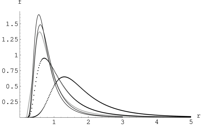
Figure 10: Final distributions of $r$ corresponding to the four most precise results on Re($\epsilon^{\prime}/\epsilon$), compared with the reference prior one (grey line), i.e. having $\mbox{E}[r_{i}]=\sigma(r_{i})=1$ $\forall i$. The continuous lines refer to the CERN results, dotted lines to the Fermilab ones.

and standard deviations of the distributions are given in Table 4, also showing the values that one would obtain with the other sets of parameters that we have considered to be edge ones.

Once more, the results are in qualitative agreement with intuition: The CERN curves are slightly squeezed below $r=1$, as the uncertainty evaluation seems to be a bit conservative. The Fermilab ones show instead some drift towards large $r$. In particular, figure and table make one suspect that some contribution to the error has been overlooked in the E731 data. Note that in this case the average value of the rescaling factor is smaller than one could expect from alternative procedures which require the overall $\chi^{2}$ to equal the number of degrees of freedom. The reason is the shape of the initial distribution of $r$, which protects us against unexpectedly large values of the rescaling factors.

Table 4: Posterior estimation of $r=\sigma_{i}/s_{i}$ starting from identical priors having $\mbox{E}_{\circ}[r]=1$ and $\sigma_{\circ}(r)=0.5$, 1.0 and 1.5. The individual results are given by $d_{i}\pm s_{i}$ to be consistent with the notation used throughout this paper.

Experiment	$d_{i}$	$s_{i}$	Posterior $\mbox{E}[r_{i}]$ $(\sigma(r_{i}))$
			$\sigma_{\circ}(r)=0.5$	$\mathbf{\sigma_{\circ}(r)=1}$	$\sigma_{\circ}(r)=1.5$
E731 (1988) [2]	32	30	0.9 (0.4)	0.8 (0.5)	0.7 (0.5)
E731 (1993)[4]	7.4	5.9	1.6 (0.7)	1.9 (1.2)	2.1 (1.5)
NA31 (1988+1993)[5, 6]	23.0	6.5	0.9 (0.4)	0.8 (0.5)	0.8 (0.6)
KTeV (1999)[7]	28.0	4.1	1.2 (0.6)	1.2 (0.9)	1.2 (1.0)
NA48 (1999)[8]	18.5	7.3	0.9 (0.4)	0.9 (0.5)	0.9 (0.6)

6 Discussion and conclusions

The problem of combining data which appear in mutual disagreement has been analysed from a probabilistic perspective. We have started from the usual hypotheses on which the well-known combination rule is based and we have seen that a possible solution can be based on a suitable modelling of the uncertainty on the standard deviation which describes the Gaussian likelihood. The complete status of uncertainty on the true value resulting from the various pieces of information is quantified by a p.d.f. $f(\mu)$ which, in our approach, does not have an a priori defined shape. This property allows one to obtain results which never conflict with the intuitive judgement of experienced physicists. The method described here also allows one to infer the ratio between the ‘true’ standard deviation and the stated one, as a result of the mutual agreement of the data.

The application of this method to CP violation results from K${}^{0}\rightarrow 2\pi$ shows that the picture of a positive and sizeable value of Re($\epsilon^{\prime}/\epsilon$) survives a sceptical analysis. This conclusion also holds if one considers separately CERN and Fermilab results. As far as a number to summarize the result is concerned, the mass of probability is concentrated around $23.5\times 10^{-4}$, with a $\pm 3.4\times 10^{-4}$ interval having a 68% probability of containing the true value. However the p.d.f. has a negative skewness that cannot be ignored. As a consequence, the expected value is slightly below the mode, at $22.7\times 10^{-4}$. We would like to re-state that what matters for uncertainty propagation is the expected value, together with the standard deviation ($3.5\times 10^{-4}$), and not the mode, or the median, and the $\pm 34\%$ probability interval around either of them.

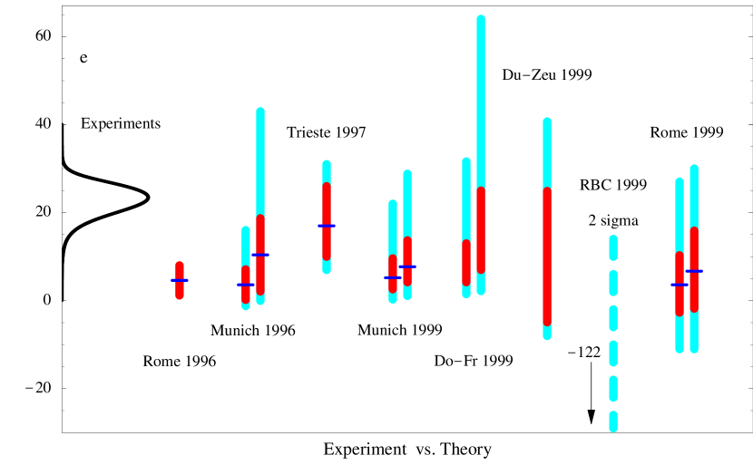
Figure 11: Combined result on Re($\epsilon^{\prime}/\epsilon$) compared with recent and very new theoretical calculations (see text).

                            [20]        [21]        [22]        [23]        [24]        [25]           [26]    [12]

The 1999 experimental results on Re($\epsilon^{\prime}/\epsilon$) have indeed renewed the interest of theorists in the subject. The comparison of the combined result with recent [20, 21, 22] and very new [23, 24, 25, 26, 12] theoretical evaluations  is given in Fig. 11, an extension of the updated version [27] of Fig. 2 of Ref. [11]. The vertical bands quantify somehow the uncertainty stated by the theoretical teams. The dark-grey bars should have the meaning of 68% central probability bands, although sometimes they are given as standard deviation of a non-Gaussian distribution. The grey bars are obtained using a procedure that the theorists call ‘scanning’ (see original papers), but which has no well-defined probabilistic meaning. Since scanning produces very pessimistic uncertainty intervals, covering values of Re($\epsilon^{\prime}/\epsilon$) which the authors hardly believe, one should be careful about concluding from Fig. 11 that the experimental value of Re($\epsilon^{\prime}/\epsilon$) is well compatible with all the approaches used to evaluate it. For example, Fig. 12,

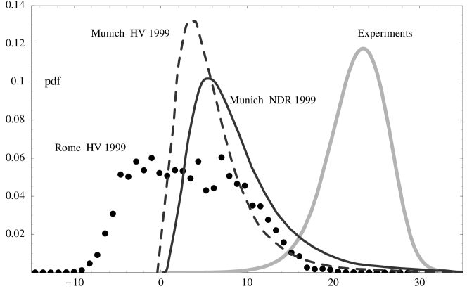
Figure 12: Probability density functions resulting from the combined experimental information about Re($\epsilon^{\prime}/\epsilon$) compared with 1999 theoretical evaluations by the Munich [23] and the Rome [12] groups (the Rome NDR evaluation is very similar to the HV one).

                                                                                                    e

which shows the p.d.f.’s of the Munich and Rome teams, alongside that obtained from the combined analysis of the experimental results, gives a better idea of the mutual compatibility, and of how to interpret the grey bars of Fig. 11 (note, in particular the positive skewness of the theory curves and negative skewness of the experiment curve). The grey-dashed bar shows the upper 2 $\sigma$ tail of the result of a recent evaluation [26] which gives a very large negative value, having also a large uncertainty.

In conclusion, it seems that, given the well-known difficulties both in the experimental determination and in the theoretical evaluation, the overall picture is not dramatically worrying (and therefore invoking new phenomenology seems premature). What it is practically certain is that direct CP violation in the neutral-kaon system is established. We are all looking forward to an accurate theoretical explanation of the effect.

References

- [1] G. D’Agostini, Report CERN 99–03, July 1999.
- [2] M. Woods et al. Phys. Rev. Lett. 60 (1988) 1695.
- [3] H. Burkhardt et al. Phys. Lett. B206 (1988) 169.
- [4] L.K. Gibbons et al. Phys. Rev. Lett. 70 (1993) 1203.
- [5] G. Barr et al. , Phys. Lett. B317 (1993) 233.
- [6] H. Wahl, private communication (for the separation in statistical and systematic contribution of the combined result).
- [7] A. Alavi-Harati et al., EFI-99-25, May 1999, hep-ex/9905060.
- [8] NA48 Collaboration, V. Fanti et al., CERN–EP99–114, August 1999, hep-ex/9909022.
- [9] H. Quinn and J. Hewett, Physics World, 12 no 5, May 1999, pp. 37–42.
- [10] A.J. Buras, TUM–HEP–355/99, August 1999, hep-ph/9908395.
- [11] M. Fabbrichesi, hep-ph/9909224, September 1999.
- [12] M. Ciuchini, E. Franco, L. Giusti, V. Lubicz and G. Martinelli, BUHEP–99–24, RM3–TH/99–9 and ROME 99/1267, October 1999, hep-ph/9910236.
- [13] U. Nierste, FERMILAB-Conf-99/288-T, October 1999, hep-ph/9910257.
- [14] V. Dose and W. von der Linden, Proc. of the XVIII International Workshop on Maximum Entropy and Bayesian Methods, Garching (Germany), July 1998, eds. V. Dose, W. von der Linden, R. Fischer, and R. Preuss, (Kluwer Academic Publishers, Dordrecht, 1999), pp. 47–56; preprint in http://www.ipp.mpg.de/OP/Datenanalyse/Publications/Papers/dose99a.ps.
- [15] G. D’Agostini, physics/9908014, August 1999, to be published in the American Journal of Physics.
- [16] C.F. Gauss, Theoria motus corporum coelestium in sectionibus conicis solem ambientium, Hamburg 1809, n.i 172–179; reprinted in Werke, Vol. 7, Herausgegeben von der Königlichen Gesellschaft der Wissenschaften zu Göttingen, (Gotha, Göttingen, 1871), pp. 225–234.
- [17] G. D’Agostini, Proc. of the XVIII International Workshop on Maximum Entropy and Bayesian Methods, Garching (Germany), July 1998, V. Dose, W. von der Linden, R. Fischer, and R. Preuss, eds. (Kluwer Academic Publishers, Dordrecht, 1999), pp. 157–170, physics/9811046.
- [18] V. Dose, private communication.
- [19] Data Particle Group, C. Caso et al., Eur. Phys. J. C3 (1998) 1.
- [20] M. Ciuchini, Nucl. Phys. B Proc. Suppl. 59 (1997) 149, and references therein.
- [21] A. Buras, M. Jamin and M.E. Lautenbacher, Phys. Lett. B389 (1996) 749.
- [22] S. Bertolini, J.O. Eeg, M. Fabbrichesi and E.I. Lashin, Nucl. Phys. B514 (1998) 93.
- [23] A.J. Buras, M. Gorbahn, S. Jäger, M. Jamin, M.E. Lautenbacher and L. Silvestrini, TUM-HEP-347/99, hep-ph/9904408.
- [24] T. Hambye, G.O. Kohler, E.A. Paschos and P.H. Soldanet, DO–TH–99–10, LNF–99/016(P), June 1999, hep-ph/9906434.
- [25] A.A. Bel’kov, G. Bohm, A.V. Lanyov and A.A. Moshkin, JINR E2–99–236, July 1999, hep-ph/99007335.
- [26] T. Blum et al. (RIKEN-BNL-Columbia Collaboration), BNL-66731, CU–TP–947, August 1999, hep-lat/9908025.
- [27] M. Fabbrichesi, private communication.