Hadronic Shower Development in Tile Iron-Scintillator Calorimetry

Abstract

The lateral and longitudinal profiles of hadronic showers detected by a prototype of the ATLAS Iron-Scintillator Tile Hadron Calorimeter have been investigated. This calorimeter uses a unique longitudinal configuration of scintillator tiles. Using a fine-grained pion beam scan at 100 GeV, a detailed picture of transverse shower behavior is obtained. The underlying radial energy densities for four depth segments and for the entire calorimeter have been reconstructed. A three-dimensional hadronic shower parametrization has been developed. The results presented here are useful for understanding the performance of iron-scintillator calorimeters, for developing fast simulations of hadronic showers, for many calorimetry problems requiring the integration of a shower energy deposition in a volume and for future calorimeter design.

1 The Calorimeter

We report on an experimental study of hadronic shower profiles detected by the prototype of the ATLAS Barrel Tile Hadron Calorimeter (Tile calorimeter) [1]. The innovative design of this calorimeter, using longitudinal segmentation of active and passive layers provides an interesting system for the measurement of hadronic shower profiles. Specifically, we have studied the transverse development of hadronic showers using 100 GeV pion beams and longitudinal development of hadronic showers using 20 – 300 GeV pion beams.

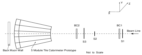
Figure 1: Schematic layout of the experimental setup (side view).

The prototype Tile Calorimeter used for this study is composed of five modules stacked in the $Y$ direction, as shown in Fig. 1. Each module spans $2\pi/64$ in the azimuthal angle, 100 cm in the $Z$ direction, 180 cm in the $X$ direction (about 9 interaction lengths, $\lambda_{I}$, or about 80 effective radiation lengths, $X_{0}$), and has a front face of 100 $\times$ 20 cm² [2]. The iron to scintillator ratio is $4.67:1$ by volume. The modules are divided into five segments along $Z$ and they are also longitudinally segmented (along $X$) into four depth segments. The readout cells have a lateral dimensions of 200 mm along $Z$, and longitudinal dimensions of 300, 400, 500, 600 mm for depth segments 1 – 4. The calorimeter was placed on a scanning table that allowed movement in any direction. Upstream of the calorimeter, a trigger counter telescope (S1, S2, S3) was installed, defining a beam spot approximately 20 mm in diameter. Two delay-line wire chambers (BC1 and BC2), each with $(Z,Y)$ readout, allowed the impact point of beam particles on the calorimeter face to be reconstructed to better than $\pm 1$ mm [3]. “Muon walls” were placed behind (800$\times$800 mm²), shown in Fig. 1 as “Back Muon Wall”, and on the positive $Z$ side (400$\times$1150 mm²), not seen in Fig. 1, of the calorimeter modules to measure longitudinal and lateral hadronic shower leakage. The data used for the study of lateral profiles were collected in 1995 during a special $Z$-scan run at the CERN SPS test beam. The calorimeter was exposed to 100 GeV negative pions at a $10^{\circ}$ angle with varying impact points in the $Z$-range from $-360$ to $200$ mm. A total of $>$ 300,000 events have been analysed. The uniformity of the calorimeter’s response for this $Z$-scan is estimated to be $1\%$ [4]. The data used for the study of longitudinal profiles were obtained using 20 – 300 GeV negative pions at a $20^{\circ}$ angle and were also taken in 1995 during the same test beam run.

2 Extracting the Underlying Radial Energy Density

There are several methods for extracting the radial density $\Phi(r)$ from the measured distributions of energy depositions. One method was used in the analysis of the data from the lead-scintillating fiber calorimeter [5]. Another method for extracting the radial density is to use the marginal density function $f(z)$ which is related to the radial density $\Phi(r)$ [6],

$$\Phi(r)=-\frac{1}{\pi}\ \frac{d}{dr^{2}}\int_{r^{2}}^{\infty}\frac{f(z)\ dz^{2}}{\sqrt{z^{2}-r^{2}}}.$$ (1)

We used the sum of three exponential functions to parameterize $f(z)$ as

$$f(z)=\frac{E_{0}}{2B}\ \sum_{i=1}^{3}\ a_{i}\ e^{-\frac{|z|}{{\lambda}_{i}}},$$ (2)

where $z$ is the transverse coordinate, $E_{0},\ a_{i},\ \lambda_{i}$ are free parameters, $B=\sum_{i=1}^{3}a_{i}\lambda_{i}$, $\sum_{i=1}^{3}a_{i}=1$ and $\int_{-\infty}^{+\infty}f(z)dz=E_{0}$. The radial density function, obtained by integration and differentiation of equation (1), is

$$\Phi(r)=\frac{E_{0}}{2\pi B}\ \sum_{i=1}^{3}\ \frac{a_{i}}{\lambda_{i}}\ K_{0}(r/\lambda_{i}),$$ (3)

where $K_{0}$ is the modified Bessel function. We define a column of five cells in a depth segment as a tower. Using the parametrization shown in equation (2), we can show that the energy deposition in a tower can be written as

$$E(z)= E_{0}-\frac{E_{0}}{B}\ \sum_{i=1}^{3}\ a_{i}{\lambda}_{i}\ \cosh(\frac{|z|}{{\lambda}_{i}})\ e^{-\frac{h}{2{\lambda}_{i}}}, for\ |z|\leq\frac{h}{2},$$ (4)

$$E(z)= \frac{E_{0}}{B}\ \sum_{i=1}^{3}\ a_{i}{\lambda}_{i}\ \sinh(\frac{h}{2\lambda_{i}})\ e^{-\frac{|z|}{{\lambda}_{i}}}, for\ |z|>\frac{h}{2},$$ (5)

where $h$ is the size of the front face of the tower along the $z$ axis.

3 Transverse Behaviour of Hadronic Showers

Figure 2: Energy depositions of 100 GeV pions in towers of depth segments 1 – 4 as a function of the $z$ coordinate: top left is for depth segment 1, top right is for depth segment 2, middle left is for depth segment 3, middle right is for depth segment 4, bottom left is for over all calorimeter. Only statistical errors are shown.

Figure 2 shows the energy depositions in towers for depth segments 1 – 4 as a function of the $z$ coordinate of the center of the tower and for entire calorimeter. Here the coordinate system is linked to the incident particle direction where $z=0$ is the coordinate of the beam impact points at the calorimeter front face. With fine parallel displacements of the beam between $-360$ mm and $200$ mm we expand the tower coordinate range from $-760$ mm to $600$ mm. To avoid edge effects, we present tower energy depositions in the range from $-650$ mm to $500$ mm. The tower energy depositions shown in Figures 2 span a range of about three orders of magnitude. The plateau for $|z|<100$ mm ($h/2$) and the fall-off at large $|z|$ are apparent. We used the distributions in Figs. 2 to extract the underlying marginal densities function for four depth segments of the calorimeter and for the entire calorimeter. The solid curves in these figures are the results of the fit with equations (4) and (5). The fits typically differ from the experimental distribution by less than $5\%$.

Table 1: The parameters $a_{i}$ and $\lambda_{i}$ obtained by fitting the transverse shower profiles for four depth segments and the entire calorimeter at 100 GeV.

$x$($\lambda_{\pi}^{Fe}$)	$a_{1}$	$\lambda_{1}$(mm)	$a_{2}$	$\lambda_{2}$(mm)	$a_{3}$	$\lambda_{3}$(mm)
0.6	$0.88\pm 0.07$	$17\pm 2$	$0.12\pm 0.07$	$48\pm 14$	$0.004\pm 0.002$	$430\pm 240$
2.0	$0.79\pm 0.06$	$25\pm 2$	$0.20\pm 0.06$	$52\pm 6$	$0.014\pm 0.006$	$220\pm 40$
3.8	$0.69\pm 0.03$	$32\pm 8$	$0.28\pm 0.03$	$71\pm 13$	$0.029\pm 0.005$	$280\pm 30$
6.0	$0.41\pm 0.05$	$51\pm 10$	$0.52\pm 0.06$	$73\pm 18$	$0.07\pm 0.03$	$380\pm 140$
all	$0.78\pm 0.08$	$23\pm 1$	$0.20\pm 0.08$	$58\pm 4$	$0.015\pm 0.004$	$290\pm 40$

The parameters $a_{i}$ and $\lambda_{i}$, obtained by fitting, are listed in Table 1. The $a_{i}$ and $\lambda_{i}$ parameters demonstrate linear behaviour as a function of $x$: $a_{i}(x)=\alpha_{i}+\beta_{i}x$ and $\lambda_{i}(x)=\gamma_{i}+\delta_{i}x$. The values of the parameters $\alpha_{i}$, $\beta_{i}$, $\gamma_{i}$ and $\delta_{i}$ are presented in Table 2.

Table 2: The values of the parameters $\alpha_{i}$, $\beta_{i}$, $\gamma_{i}$ and $\delta_{i}$.

	$\alpha_{i}$	$\beta_{i}$ ($1/\lambda_{\pi}$)		$\gamma_{i}$ (mm)	$\delta_{i}$ ($\mathrm{mm}/\lambda_{\pi}$)
$a_{1}$	$0.99\pm 0.06$	$-0.088\pm 0.015$	$\lambda_{1}$	$13\pm 2$	$6\pm 1$
$a_{2}$	$0.04\pm 0.06$	$0.071\pm 0.015$	$\lambda_{2}$	$42\pm 10$	$6\pm 4$
$a_{3}$	$-0.001\pm 0.002$	$0.008\pm 0.002$	$\lambda_{3}$	$170\pm 80$	$29\pm 23$

4 Radial Hadronic Shower Energy Density

Using formula (3) and the values of the parameters $a_{i}$, $\lambda_{i}$, given in Table 1, we have determined the underlying radial hadronic shower energy density functions, $\Phi(r)$. The results are shown in Figure 3 for depth segments 1 – 4 and for the entire calorimeter. The contributions of the three terms of $\Phi(r)$ are also shown.

Figure 3: Radial energy density, $\Phi(r)$, as a function of $r$ for Tile calorimeter for depth segments 1 – 4: top left is for depth segment 1, top right is for depth segment 2, middle left is for depth segment 3, middle right is for depth segment 4, bottom left is for entire calorimeter. The solid lines are the energy densities $\Phi(r)$, the dashed lines are the contribution from the first term from, the dash-dotted lines are the contribution from the second term, the dotted lines are the contribution from the third term. Bottom right: Comparison of the radial energy densities as a function of $r$ (in units of $\lambda_{\pi}^{eff}$) for Tile calorimeter (the solid line) and lead-scintillating fiber calorimeter (the dash-dotted line).

The function $\Phi(r)$ for the entire calorimeter has been compared with the one for the lead-scintillating fiber calorimeter of Ref. [5], that has about the same effective nuclear interaction length for pions [6]. The two radial density functions are rather similar as seen in Fig. 3 (bottom right). The lead-scintillating fiber calorimeter density function $\Phi(r)$ was obtained from a 80 GeV $\pi^{-}$ grid scan at an angle of $2^{\circ}$ with respect to the fiber direction. For the sake of comparing the radial density functions of the two calorimeters, the distribution from [5] was normalised to the $\Phi(r)$ of the Tile calorimeter. Precise agreement between these functions should not be expected because of the effect of the different absorber materials used in the two detectors, the values of $e/h$ are different, as is hadronic activity of showers because fewer neutrons are produced in iron than in lead.

5 Radial Containment

The parametrization of the radial density function, $\Phi(r)$, was integrated to yield the shower containment as a function of the radius $I(r)=E_{0}-\frac{E_{0}r}{B}\ \sum_{i=1}^{3}\ a_{i}\ K_{1}(r/{\lambda}_{i})$, where $K_{1}$ is the modified Bessel function. The approximation of the data for the radii of cylinders for given shower containment ($90\%$, $95\%$ and $99\%$) as a function of depth with linear fits are $r(90\%)=(85\pm 6)+(37\pm 3)x$, $r(95\%)=(134\pm 9)+(45\pm 3)x$, $r(99\%)=(349\pm 7)+(22\pm 2)x$ (mm). The centers of depth segments, $x$, are given in units of $\lambda_{\pi}^{Fe}$.

6 Longitudinal Profile

Figure 4: Top: The longitudinal profile (circles) of the hadronic shower at 100 GeV as a function of the longitudinal coordinate $x$ in units of $\lambda_{\pi}^{Fe}$. Open triangles are data from the calorimeter of Ref.⁷ diamonds are the Monte Carlo (GEANT-FLUKA) predictions. The dash-dotted line is the fit by function (6), the solid line is calculated with function (7) with parameters from Ref.⁷ the dashed line is calculated with function (7) with parameters from Ref.⁸ The electromagnetic and hadronic components of the shower (crosses and squares), together with their fits using (6), are discussed in Section 8. Bottom: Longitudinal profiles of the hadronic showers from 20 GeV (open stars), 50 GeV (open squares) and 100 GeV (open circles) pions as a function of the longitudinal coordinate $x$ in units of $\lambda_{I}$ for a conventional iron-scintillator calorimeter ⁷ and of 20 GeV (black stars), 50 GeV (black squares), 100 GeV (black circles), 150 GeV (black up triangles), 200 GeV (asterisks), 300 GeV (black down triangles) for pions at $20^{\circ}$ and of 100 GeV (black circles) for pions at $10^{\circ}$ for Tile iron-scintillator calorimeter. The solid lines are calculated with function (7) with parameters from Ref.⁷ and the dashed lines are with parameters from Ref.⁸

Our values of $\Delta E/\Delta x$ together with the data of [7] and Monte Carlo predictions (GEANT-FLUKA + MICAP) [9] are shown in Fig. 4 (top). The longitudinal energy deposition for our calorimeter is in good agreement with that of a conventional iron-scintillator calorimeter. The longitudinal profile may be approximated using two parametrizations. The first form is

$$\frac{dE(x)}{dx}=\frac{E_{f}\ \beta^{\alpha+1}}{\Gamma(\alpha+1)}\ x^{\alpha}\ e^{-\beta x}$$ (6)

where $E_{f}=E_{beam}$, and $\alpha$ and $\beta$ are free parameters. Our data at 100 GeV and those of Ref. [7] at 100 GeV were jointly fit to this expression; the fit is shown in Fig. 4 (top). The second form is the analytical representation of the longitudinal shower profile from the front of the calorimeter

$$\frac{dE(x)}{dx} = N\ \Biggl{\{}\frac{w\ X_{0}}{a}\ \biggl{(}\frac{x}{X_{0}}\biggr{)}^{a}\ e^{-b\frac{x}{X_{0}}}\ {}_{1}F_{1}\biggl{(}1,\ a+1,\ \biggl{(}b-\frac{X_{0}}{\lambda_{I}}\biggr{)}\ \frac{x}{X_{0}}\biggr{)}$$ (7)

$$+\ \frac{(1-w)\ \lambda_{I}}{a}\ \biggl{(}\frac{x}{\lambda_{I}}\biggr{)}^{a}\ e^{-d\frac{x}{\lambda_{I}}}\ {}_{1}F_{1}\biggl{(}1,\ a+1,\ \bigl{(}d-1\bigr{)}\ \frac{x}{\lambda_{I}}\biggr{)}\Biggr{\}},$$

where $a,\ b,\ d,\ w$ are parameters, ${}_{1}F_{1}$ is the confluent hypergeometric function. Here the depth variable, $x$, is the depth in equivalent $Fe$, $X_{0}$ is the radiation length in $Fe$ and in this case $\lambda_{I}$ is $\lambda_{\pi}^{Fe}$. The normalisation factor $N=E_{beam}/\lambda_{I}\ \Gamma(a)\ (w\ X_{0}\ b^{-a}+(1-w)\ \lambda_{I}\ d^{-a})$. This form was suggested in [10] and derived by integration over the shower vertex positions of the longitudinal shower development from the shower origin. For the parametrization of longitudinal shower development from the shower origin, the well known parametrization suggested by Bock et al. [8] has been used. We compare the form (7) to the experimental points at 100 GeV using the parameters calculated in Refs. [8] and [7]. Note that now we are not performing a fit but checking how well the general form (7) together with two sets of parameters for iron-scintillator calorimeters describe our data. As shown in Fig. 4 (top), both sets of parameters work rather well in describing the 100 GeV data. Turning next to the longitudinal shower development at different energies, in Fig. 4 (bottom) our values of $\Delta E/\Delta x$ for 20 – 300 GeV together with the data from [7] are shown. The solid and dashed lines are calculations with function (7) using parameters from [7] and [8], respectively. Again, we observe reasonable agreement between our data and the corresponding data for conventional iron-scintillator calorimeter on one hand, and between data and the parametrizations described above. Note that the fit in [7] has been performed in the energy range from 10 to 140 GeV; hence the curves for 200 and 300 GeV should be considered as extrapolations. It is not too surprising that at these energies the agreement is significantly worse, particularly at 300 GeV. In contrast, the parameters of [8] were derived from data spanning the range 15 – 400 GeV, and are in much closer agreement with our data.

7 The parametrization of Hadronic Showers

The three-dimensional parametrization for spatial hadronic shower development is

$$\Psi(x,r)=\frac{dE(x)}{dx}\cdot\frac{\sum_{i=1}^{3}\ \frac{a_{i}(x)}{\lambda_{i}(x)}\ K_{0}\bigl{(}\frac{r}{\lambda_{i}(x)}\bigr{)}}{2\pi\ \sum_{i=1}^{3}a_{i}(x)\lambda_{i}(x)}\ ,$$

where $dE(x)/dx$, defined by equation (7), is the longitudinal energy deposition.

8 Electromagnetic Fraction of Hadronic Showers

Figure 5: The fraction $f_{\pi^{0}}$ in hadronic showers versus the beam energy. The star is our data, the solid curve is the Groom parametrization, the dashed curve is the Wigmans parametrization, squares are the GEANT-CALOR predictions, circles are the GEANT-GHEISHA predictions and crosses are the CALOR predictions.

Following [5], we assume that the electromagnetic part of a hadronic shower is the prominent central core, which in our case is the first term in the expression (3) for the radial energy density function, $\Phi(r)$. Integrating $f_{\pi^{0}}$ over $r$ we get $f_{\pi^{0}}=a_{1}\lambda_{1}/\sum_{i=1}^{3}a_{i}\lambda_{i}$. For the entire Tile calorimeter this value is $(53\pm 3)\%$ at 100 GeV. The observed $\pi^{0}$ fraction, $f_{\pi^{0}}$, is related to the intrinsic actual fraction, $f^{\prime}_{\pi^{0}}$, by the equation $f_{\pi^{0}}(E)=\frac{e\ E^{\prime}_{em}}{e\ E^{\prime}_{em}+h\ E^{\prime}_{h}}=\frac{e/h\cdot f^{\prime}_{\pi^{0}}(E)}{(e/h-1)\cdot f^{\prime}_{\pi^{0}}(E)+1}$, where $E^{\prime}_{em}$ and $E^{\prime}_{h}$ are the intrinsic electromagnetic and hadronic parts of shower energy, $e$ and $h$ are the coefficients of conversion of intrinsic electromagnetic and hadronic energies into observable signals, $f^{\prime}_{\pi^{0}}=E^{\prime}_{em}/(E^{\prime}_{em}+E^{\prime}_{h})$. There are two analytic forms for the intrinsic $\pi^{0}$ fraction suggested by Groom [11] $f^{\prime}_{\pi^{0}}(E)=1-(E/E_{0}^{\prime})^{m-1}$ and Wigmans [12] $f^{\prime}_{\pi^{0}}(E)=k\cdot ln{(E/E_{0}^{\prime})}$, where $E_{0}^{\prime}=1$ GeV, $m=0.85$ and $k=0.11$. We calculated $f_{\pi^{0}}$ using the value $e/h=1.34\pm 0.03$ for our calorimeter [13] and obtained the curves shown in Fig. 5. Our result at 100 GeV is compared to the modified Groom and Wigmans parametrizations and to results from the Monte Carlo codes CALOR [14], GEANT-GEISHA and GEANT-CALOR (the latter code is an implementation of CALOR89 differing from GEANT-FLUKA only for hadronic interactions below 10 GeV). As can be seen from Fig. 5, our calculated value of $f_{\pi^{0}}$ is about one standard deviation lower than two of the Monte Carlo results and the Groom and Wigmans parametrizations. The fractions $f_{\pi^{0}}(r)$ for the entire calorimeter and for depth segments 1 – 3 amount to about $90\%$ as $r\rightarrow 0$ and decrease to about $1\%$ as $r\rightarrow\lambda_{\pi}^{eff}$. However for depth segment 4 the value of $f_{\pi^{0}}(r)$ amounts to only $50\%$ as $r\rightarrow 0$ and decreases slowly to about $10\%$ as $r\rightarrow\lambda_{\pi}^{eff}$. The values of $f_{\pi^{0}}(x)$ as a function of $x$ are fitted by $f_{\pi^{0}}(x)=(75\pm 2)-(8.4\pm 0.4)x$ ($\%$). Using the values of $f_{\pi^{0}}(x)$ and energy depositions for various depth segments, we obtained the contributions from the electromagnetic and hadronic parts of hadronic showers in Fig. 4 (top). The curves represent a fit to the electromagnetic and hadronic components of the shower using equation (6). $E_{f}$ is set equal to $f_{\pi^{0}}E_{beam}$ for the electromagnetic fraction and $(1-f_{\pi^{0}})E_{beam}$ for the hadronic fraction. The electromagnetic component of a hadronic shower rise and decrease more rapidly than the hadronic one ($\alpha_{em}=1.4\pm 0.1$, $\alpha_{h}=1.1\pm 0.1$, $\beta_{em}=1.12\pm 0.04$, $\beta_{h}=0.65\pm 0.05$). The shower maximum position ($x_{max}=(\alpha/\beta)\ \lambda_{\pi}^{Fe}$) occurs at a shorter distance from the calorimeter front face ($x_{max}^{em}=1.23\ \lambda_{\pi}^{Fe}$, $x_{max}^{h}=1.85\ \lambda_{\pi}^{Fe}$). At depth segments greater than $4\ \lambda_{\pi}^{Fe}$, the hadronic fraction of the shower begins to dominate. This is natural since the energy of the secondary hadrons is too low to permit significant pion production.

9 Summary and Conclusions

We have investigated the lateral development of hadronic showers using 100 GeV pion beam data at an incidence angle of $\Theta=10^{\circ}$ for impact points $z$ in the range from $-360$ to $200$ mm and the longitudinal development of hadronic showers using 20 – 300 GeV pion beams at an incidence angle of $\Theta=20^{\circ}$. We have obtained for four depth segments and for the entire calorimeter: energy depositions in towers; underlying radial energy densities; the radii of cylinders for a given shower containment fraction; the fractions of the electromagnetic and hadronic parts of a shower; differential longitudinal energy deposition. The three-dimensional parametrization of hadronic showers that we obtained allows direct use in any application that requires volume integration of shower energy depositions and position reconstruction.

10 Acknowledgements

This paper is the result of the efforts of many people from the ATLAS Collaboration. The authors are greatly indebted to the entire Collaboration for their test beam setup and data taking. We are grateful to the staff of the SPS, and in particular to Konrad Elsener, for the excellent beam conditions and assistance provided during our tests.

References

• [1] ATLAS Tile Calorimeter Technical Design Report, CERN/LHCC/96-42.
• [2] E.Β Berger $et\ al.$, CERN/LHCC 95-44, CERN, Geneva, Switzerland, 1995.
• [3] F.Β Ariztizabal $et\ al.$, NIM A349 (1994) 384.
• [4] J.A.Β Budagov, Y.A.Β Kulchitsky $et\ al.$, JINR, E1-96-180, Dubna, 1996.
• [5] D.Β Acosta $et\ al.$, NIM A316 (1992) 184.
• [6] J.A.Β Budagov, Y.A.Β Kulchitsky $et\ al.$, JINR, E1-97-318, Dubna, 1997.
• [7] E.Β Hughes, Proc.Β of the I Int.Β Conf.Β on Calor.Β in HEP, p.525, USA, 1990.
• [8] R.K.Β Bock $et\ al.$, NIM 186 (1981) 533.
• [9] A.Β Juste, ATLAS Note, TILECAL-No-69, CERN, 1995.
• [10] Y.A.Β Kulchitsky, V.B.Β Vinogradov, NIM A413 (1998) 484.
• [11] D.Β Groom, Proc., Cal.Β for the Supercollider, USA, 1990.
• [12] R.Β Wigmans, NIM A265 (1988) 273.
• [13] J.A.Β Budagov, Y.A.Β Kulchitsky $et\ al.$, JINR, E1-95-513, Dubna, 1995.
• [14] T.A.Β Gabriel $et\ al.$, NIM A338 (1994) 336.