Current Performance of the SLD VXD3

Abstract

During 1996, the SLD collaboration completed construction and began operation of a new charge-coupled device (CCD) vertex detector (VXD3). Since then, its performance has been studied in detail and a new topological vertexing technique has been developed. In this paper, we discuss the design of VXD3, procedures for aligning it, and the tracking and vertexing improvements that have led to its world-record performance.

Presented at 8th International Workshop on Vertex Detectors (VERTEX 99),
The Netherlands, 20-25 June 1999.

1 Introduction

A technique of charge-coupled device (CCD) detectors for high energy experiments was established by the NA32 fixed-target experiment at CERN in mid 80s [1]. They used a CCD-based vertex detector for the identification of charmed particles. Their results showed excellent vertexing performance for short-lived particles. It was realized that these devices offered the possibility of excellent physics performance in the $e^{+}e^{-}$ linear collider environment. The SLD experiment at the SLAC Linear Collider (SLC) is the first experiment which uses CCDs as a vertex detector in a colliding beam experiment. After tests with a prototype detector VXD1, the 120M pixel detector VXD2 [2, 3] was installed for physics runs starting in January 1992. During the SLD runs with VXD2, we developed a topological vertex finding algorithm [4] to tag heavy-quark jets. The very small ($\mu\mathrm{m}$ size) and stable SLC interaction point (IP) and cleanly and precisely measured space points ($\sim 5.4\mu\mathrm{m}$) in VXD2 permit efficient identification of secondary and even tertiary vertices. With VXD2 and this technique, we enjoyed an advantage in both $b$- and $c$-jet tagging [5] over other collider experiments.

Rapid advances in CCD technology over the past 10 years made it possible to replace VXD2 with a much more powerful vertex detector. The upgraded vertex detector is called VXD3 [6] and was installed in December 1995. VXD3 provides much better impact parameter resolution, larger solid angle coverage, and virtually error-free track linking. All these features enhance the SLD heavy-quark measurements. One of the most exciting possibilities is the search for $B^{0}_{s}$ mixing, leading to the measurement of the oscillation frequency, $\Delta m_{s}$, and an improved determination of the CKM matrix element, $V_{td}$. The initial performance of VXD3 can be found in Refs. [6, 7, 8]. Since then, significant improvements in alignment and tracking algorithms have led to remarkable performance results.

In this paper, we report the current performance of the SLD VXD3. The features of CCD vertex detectors and VXD3 are described in Section 2. Section 3 discusses the alignment correction for precise space point determination and current achieved spatial resolution. In Section 4, we present the VXD3-aided track finder which improves the solid angle coverage of track reconstruction at SLD. Section 5 describes the track-fitter improvement and a new topological vertexing technique. Our latest impact parameter resolution and topological vertexing performances are also shown in this section. Finally a summary is given in Section 6.

2 The SLD VXD3

CCD-based vertex detectors are well matched to $e^{+}e^{-}$ linear colliders, providing nearly ideal experimental conditions for heavy flavor physics, for the following reasons:

1. Very small beam spots ($\mu\mathrm{m}$ size), hence a well defined primary vertex for every event.

2. Highly segmented pixel structure, which provides natural 3-dimensional space points and would comfortably absorb high background per bunch crossing, likely to be found in a linear collider.

3. Precise space-point resolution, resulting to date in a measurement precision of $<4\mu\mathrm{m}$ in space points.

4. Very thin detectors and small beam pipe radius, hence degradation of impact parameter resolution due to multiple scattering could be greatly reduced.

5. Long interval between bunch crossings. While this is not sufficient for complete readout, the average integrated background during readout was only $\sim 10$ bunch crossings.

The SLD experiment is the only collider experiment which satisfies the above conditions. The detailed description of VXD3 is found in Ref. [6]. Using advances in CCD technology, in particular increasing the device active area, VXD3 has the following features:

1. Extended polar angle coverage, to benefit from the large polarized asymmetry in physics processes in the most valuable regions of high $|\cos\theta|$.

2. Full azimuthal coverage in each of three barrels, to achieve redundancy and self-tracking capability independent of the Central Drift Chamber (CDC), and consequently improved overall tracking efficiency.

3. Optimized geometry with stretched radial lever arm and reduced material in each layer, for significantly improved impact parameter resolution.

VXD3 consists of 96 CCDs [9] arranged on 3 cylindrical layers of beryllium supporting ladders around the interaction point (IP). Only 2 CCDs cover the entire length of the 159mm ladder with an overlap of about 1mm in the region near $z=0$, see Fig. 1a. Ladders in the same layer are placed in a ‘shingled’ layout with a small cant angle of $9-10^{\circ}$. The layout provides azimuthal coverage overlap in the range of $300\mu\mathrm{m}$ to 1mm, depending on layer and CCD location, see Fig. 1b. The overlaps allow an internal detector alignment by using the tracks passing through the overlap regions, discussed in Section 3. With a beam pipe inner radius of 23.5mm and the layer-1 radius of 28.0mm, the layer-3 radius of 48.3mm achieves complete azimuthal coverage out to $|\cos\theta|<0.85$ for $\geq 3$ VXD hits and provides enough lever arm for an accurate measurement of track angles. If 2 VXD hits are permitted, the layer-2 radius of 38.2mm allows an extend coverage of $|\cos\theta|<0.90$ (see Section 4).

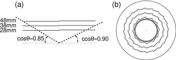
Figure 1: Layout of the CCDs in VXD3, (a) in views along the beam direction and (b) transverse.

The CCDs are n-buried channel devices fabricated on p-type epitaxial layer and having a p+ substrate. The transverse pixel sizes are $20\mu\mathrm{m}\times 20\mu\mathrm{m}$, and the epitaxial layer is 20 $\mu\mathrm{m}$ thick. They have an active area of $80\mathrm{mm}\times 16\mathrm{mm}$. Each CCD contains $4000\times 800=3.2\mathrm{M}$ pixels, so there are $3.2\mathrm{M}\times 96=307\mathrm{M}$ pixels in VXD3. They are operated in a full-frame readout mode. The readout register operates on two-phase clocking and the imaging area on three-phase. There are 4 readout nodes, one on each corner of each CCD device, and the pixel readout rate is 5 MHz. With beryllium motherboard stiffeners and the CCDs thinned to $150\mu\mathrm{m}$, a VXD3 ladder is $0.4\mathrm{\%}$ radiation lengths thick. Extended layer to layer distance arms and reduced detector material improves impact parameter resolution significantly compared to VXD2, as discussed in Section 5.

3 Alignment and spatial resolution

We expected VXD3 to give an excellent intrinsic hit resolution of $\sim 4\mu\mathrm{m}$. However, without a detailed internal alignment of the detector as installed in SLD, the average position resolution was about 4 times worse ($>16\mu\mathrm{m}$), based on an initial optical survey of VXD3 performed during its assembly. This indicates that a precise calibration is needed to achieve the full physics potential of the device. The effective single hit resolution is the product of the intrinsic resolution and the systematic uncertainties in the spatial locations and orientations of the CCDs themselves. The aim of the internal alignment is to remove the latter contribution. In order to remove the uncertainty due to the orientations of the CCDs, we use the charged track data itself. This section describes the techniques used to align the CCDs and obtain design performance [10].

In order to correct the alignment systematics, we introduce 6 parameters per CCD as a first order correction. The parameters consist of three translations and three rotations. There are a total of $6\times 96$ corrections for these degrees of freedom. In addition, a pair of parameters are introduced for the deviation of the interaction point from the nominal.

During the assembly of VXD3, the relative positions of the CCDs within each barrel of VXD3 were measured with typically a few 10s of $\mu\mathrm{m}$ precision in a room-temperature optical survey. This survey geometry forms the starting point with which the first data was reconstructed. The alignment procedure assumed that each CCD was approximately flat, with small shape corrections as measured in the optical survey.

Misalignments of CCDs cause a measured hit on a CCD to be displaced from a true track trajectory by a residual $\delta$. Even though we correct the translations, the rotations and the initial CCD shape, higher order systematics exist in the track residual distributions. We ascribe these systematics to CCD shape changes after the installation, cooling and/or imperfections in the original optical survey. These deviations can be approximated by a 4th-order polynomial along the $z$ direction. Fixing the deviations at the CCD edges to be 0, we introduce 3 additional alignment parameters per CCD to correct these higher order systematics. The alignment parameters significantly correct the radial position of a hit point on the CCD which is particularly important at large $|\cos\theta|$. Now we have 9 alignment parameters per CCD and there are $9\times 96+2=866$ alignment parameters in total.

Since the true track trajectory is unknown it is necessary to identify hits on at least three CCDs associated with a track reconstructed in CDC. We use only the measured momentum from the CDC track to constrain the track extrapolation inside VXD3. Good quality tracks are selected with a momentum of at least 1 GeV. In general the track is constrained to pass through two of the CCD hits and the corresponding residual measured the third, reference, CCD. According to combinations of three of CCDs, we classify groups of residuals, shingles, doublets, triplets, pairs and so on [12]. The small curvature effect of the charged track in the SLD magnetic field is taken into account in the $r\phi$ plane.

For each type of residual and each unique combination of CCDs data files are accumulated containing the deviations $\delta$ in $r\phi$ and $rz$ as a function of $\tan\lambda$ and $\phi$, where $\tan\lambda$ is a dip angle. These data files are fitted to the function forms such as Eq. 1, to determine the parameters of the deviations ($C_{1}$, $C_{2}$, $\ldots$) and the error matrix of these parameters.

$$\delta=C_{1}+C_{2}\tan\lambda+C_{3}\tan^{2}\lambda\ldots$$ (1)

These fits are done using MINUIT [11] with an automated procedure to loop over the large number (${\sim}1500$) of residual type/CCD combinations involved.

By inspection it is now possible for each residual type to build matrices of the form A x = c where x is a column matrix of the degrees of freedom, c is a column matrix of parameters from the functional forms of the deviations and A is a weight matrix determined by the nominal geometry. Clearly the vector x must be common to all classes, since this is simply the corrections to the CCD positions needed to optimize the geometry, so that the matrices from the different classes can be combined as illustrated in Fig. 2. The values of alignment parameters can simply be obtained by inverting the matrix A [13],

$$\mathbf{x}=\mathbf{A}^{-1}\mathbf{c}.$$ (2)

Figure 2: Schematic of the alignment matrix equation.

Fig. 3 shows an example of the detector resolution obtained with the final geometry using all events recorded in the $1997-98$ data. From these results, we obtain a consistent one-hit resolution of $\sim 3.8\mu\mathrm{m}$.

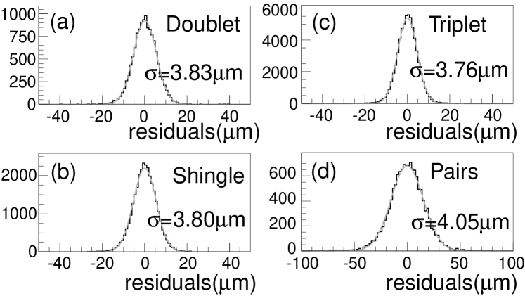
Figure 3: Residual distributions for (a) doublet, (b) shingle, (c) triplet and (d) pairs. The definition of these can be found in Ref. [12]. Fitting a Gaussian curve to each of these figures yields a width of $5.42\mu\mathrm{m}$ ,$5.37\mu\mathrm{m}$, $4.61\mu\mathrm{m}$ and $15.27\mu\mathrm{m}$ for doublets, shingles, triplets and pairs, respectively, corresponding to spatial resolutions of $3.83\mu\mathrm{m}$, $3.80\mu\mathrm{m}$, $3.76\mu\mathrm{m}$ and $4.05\mu\mathrm{m}$. One hit resolution is consistently $\sim 3.8\mu\mathrm{m}$.

It should be noted that this procedure does not need to be iterated. This is expected given the relatively minor nature of the approximations made in the analysis and is confirmed to be correct for the VXD3 geometry during 1996 data taking where a second iteration of the procedure produce no significant change to the geometry.

4 Improved solid angle coverage

Many of the SLD physics analyses (particularly the $b$ mixing and fermion asymmetry measurements) can benefit from an extended polar angle coverage, due to the large analyzing power at high $|\cos\theta|$.

The tracking strategy adopted for VXD2 was to reconstruct the CDC track first, extrapolate it to the VXD and then search for the best VXD-hit combination to form the complete track. However, Monte Carlo studies indicate that around 5% of the prompt tracks in a hadronic $Z^{0}$ decay within the CDC active volume are either not tracked by CDC or fail linking to the VXD, mainly due to contamination of wrong CDC hits distorting the extrapolation. This is a consequence of track merging in a dense hadronic jet environment, compounded by the relatively small CDC outer radius and a rather moderate solenoid field of 0.6 Tesla. This problem becomes progressively worse once the track $|\cos\theta|$ increases beyond 0.7, when the available tracking length is shortened. Actually the linking efficiency with $\geq$2 VXD hits begins to decrease at $|\cos\theta|=0.7$ and falls to $50\mathrm{\%}$ at $|\cos\theta|=0.75$. VXD2 could not offer independent assistance to relieve these pattern recognition deficiencies.

VXD3 was designed to have a full 3 layer coverage as sketched in Fig 1, allowing a self tracking within VXD3 alone. For the majority of VXD3 tracks with $\geq 3$ hits, a VXD-hit vector is relatively easy to reconstruct stand alone, while fake combinations only amount to less than $10\mathrm{\%}$ of all vectors before any matching with CDC tracks. The VXD-hit vectors have the following nice features:

1. High precision vectors: The very fine granularity of the CCD pixels is ideal for resolving the otherwise difficult merging track cases and discrimination of tracks which are case together. These high precision VXD-hit vectors in 3-D are powerful additions to the global tracking pattern recognition capability.

2. Wide acceptance: A full azimuthal and extended polar angle coverage of VXD3 guarantees to form VXD-hit vectors widely with high and flat reconstruction efficiency. For $\geq$3-VXD-hit vectors, they can be reconstruct out to $\cos\theta=0.85$, beyond the VXD2 acceptance of $|\cos\theta|<0.75$.

The VXD-hit vectors are hence quite useful in improving the tracking performance in the forward region.

The new tracking strategy adopted for VXD3 uses vertex-detector-hit vectors at the earliest stage of the track finding algorithm. The global tracking pattern recognition combines both VXD- and CDC-hit vectors into a set of tracks. Due to the 3 dimensional nature and fine segmentation of CCD pixel device, the real combinations of VXD- and CDC-hit vectors stand out clearly and fakes are easily rejected with a $\chi^{2}$ test. To form complete tracks, a joint fit the selected vectors is performed as described in Section 5. Some track are lost in the above procedure because of a kink at the boundary between VXD3 and CDC. In order to recover these tracks, CDC-alone tracks are also reconstructed and extrapolated to the VXD3 to search for the best remaining VXD-hit combination.

Since the new tracking algorithm works well with 3-VXD-hit vectors, we extend it to a more aggressive prospect, 2-VXD-hit vectors. Using the 2-VXD-hit vectors, we get an angular range of $0.85<|\cos\theta|<0.9$, beyond the coverage of 3-VXD-hit vectors. However the purity of 2-VXD-hit vectors ($=\mbox{number of signal vectors}/\mbox{number of total vectors}$) is not so high, and depends on a beam condition. In 1997 run, the purity of 2-VXD-hit vectors is typically $35\mathrm{\%}$, while that for 3-VXD-hit vectors is $93\mathrm{\%}$. The low purity results in a rather low purity of reconstructed tracks and increased CPU time.

In order to improve the purity, we look at the pulse height information of clusters in 2-VXD-hit vectors. We assume that the pulse heights depend on the path length of the charged particle in the CCD:

$$\mbox{Pulse Height}\propto\frac{\mbox{Thickness of CCD}}{\sin\theta}.$$ (3)

Fig. 4 illustrates the pulse height distributions versus $\cos\theta$ for VXD clusters associated with tracks and for all VXD clusters. According to the results of Fig. 4, we require the pulse height of VXD cluster to be greater than $14/\sin\theta$. The cut removes half of the fake 2-VXD-hit vectors. Once the purity is improved, 2-VXD-hit vectors significantly improve the forward tracking. The detailed internal alignment and the high spatial resolution allow the 2-VXD-hit vectors to determine the track direction and $z$ position accurately. In the region of $0.85<|\cos\theta|<0.9$, CDC has too few hits to determine these quantities reliably. Therefore it is very difficult to reconstruct high quality tracks in the forward region without 2-VXD-hit vectors.

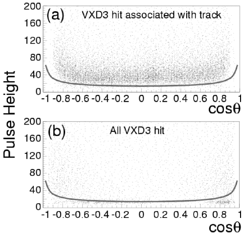
Figure 4: Pulse height distributions as a function of $\cos\theta$ for (a) VXD3 clusters associated with tracks and (b) all VXD3 clusters. The lines indicate pulse height cut requiring $>14/\sin\theta$. Signal pulse heights are above the line, while noise ones bunch below the line.

Detailed Monte Carlo simulations are used to test the tracking performance. Fig. 5a shows tracking efficiencies with $\geq 2$ VXD hits using the new track reconstruction algorithm with VXD3 and original reconstruction with VXD2, in hadron events. Significant improvement can be seen in the region of $|\cos\theta|>0.7$ and the efficiency is flat to $|\cos\theta|=0.85$ and reasonably well to near 0.9. The track purity curve is shown in Fig. 5b. The curve is uniformly high out to $|\cos\theta|=0.9$.

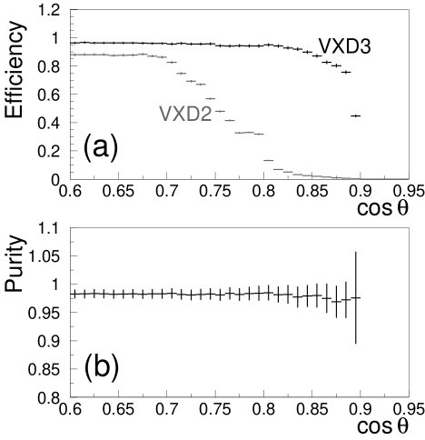
Figure 5: (a) The tracking efficiency curves as a function of $|\cos\theta|$ requiring $\geq$ 2 VXD hits. Black point indicates new track reconstruction algorithm with VXD3 and grey one original track reconstruction with VXD2. (b) The track purity curve versus $|\cos\theta|$ with new track reconstruction algorithm and VXD3.

5 Track fitter improvement and new topological vertexing technique

Track fitting procedures have also been modified. We introduce a new track extrapolation program to give more precise track reconstruction and a Kalman filter algorithm [14, 15, 16] for CDC+VXD fit $\chi^{2}$ calculation taking into account the effect of multiple scattering in detector material more accurately than before. During this process, we also discovered, and corrected, that the VXD3 cluster errors were not correctly assigned in the tracking code. Fig. 6 shows $\mu$-pair miss distance distributions in $r\phi$ and $rz$ projections. Fitting a Gaussian curve to each figure yields a width of $11.0\mu\mathrm{m}$ and $13.7\mu\mathrm{m}$ for $r\phi$ and $rz$ projections respectively. These numbers are divided by the geometric factor $\sqrt{2}$ and obtain the impact parameter resolutions of

$$\begin{array}[]{lll}\sigma_{r\phi}=7.8\mu\mathrm{m}&\sigma_{rz}=9.7\mu\mathrm{m}&\mbox{ (new track fitter with VXD3)}\\ \sigma_{r\phi}=10.7\mu\mathrm{m}&\sigma_{rz}=23.5\mu\mathrm{m}&\mbox{(original track fitter with VXD3)}\\ \sigma_{r\phi}=11\mu\mathrm{m}&\sigma_{rz}=38\mu\mathrm{m}&\mbox{(original track fitter with VXD2)}.\\ \end{array}$$

Here impact parameter resolutions by original track fitter with VXD3 and with VXD2 are also shown. With the detailed internal alignment, significant improvement can be seen, in particular $rz$ projections because we put more weight on VXD3 than CDC which has worse position resolution in $z$ direction, in the track fitter. Current impact parameter resolutions as a function of momentum and angle with VXD3 are:

$$\sigma_{r\phi}=7.8\oplus\frac{33}{p\sin^{3/2}\theta}\;\mu\mathrm{m}$$ (4)

$$\sigma_{rz}=9.7\oplus\frac{33}{p\sin^{3/2}\theta}\;\mu\mathrm{m}.$$ (5)

Our impact parameter resolution is outstanding compared with the other collider experiments.

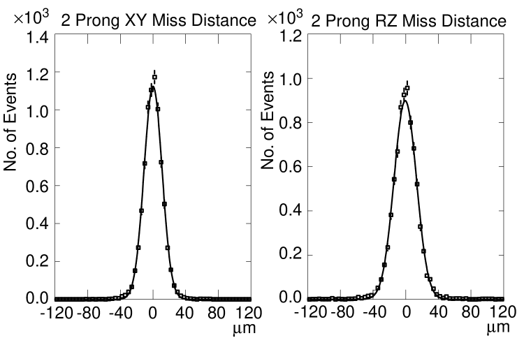
Figure 6: $\mu$-pair miss distances in $r\phi$ and $rz$ projections. The fitted $\sigma$’s correspond to impact parameter resolutions of $7.8\mu\mathrm{m}$ and $9.7\mu\mathrm{m}$. Comparing the old impact parameter resolutions of $10.7\mu\mathrm{m}$ ($23.5\mu\mathrm{m}$) in $r\phi$ ($rz$), significant improvement is seen in $\sigma_{rz}$.

Taking advantage of this significant improvement, we have developed a new algorithm to reconstruct $B$ decay. The new algorithm relies on the long $B$ and $D$ lifetimes and the kinematic fact that the large boost of the $B$ decay system carries the cascade charm decay downstream from the $B$ decay vertex. Monte Carlo studies show that in $B$ decays producing a single $D$ meson the cascade $D$ decays on average $4200\mu\mathrm{m}$ from the IP, while the intermediate $B$ vertex is displaced on average only $46\mu\mathrm{m}$ transversely from the line joining the IP to the $D$ decay vertex. This kinematic stretching of the $B$ decay chain into an approximately straight line is exploited by what is called the ghost track algorithm [17]. This new algorithm has two stages and operates on a given set of selected tracks in a jet or hemisphere. Firstly, the best estimate of the straight line from the IP directed along the $B$ decay chain is found. This line is promoted to the status of a track by assigning it a finite width. This new track, regarded as the resurrected image of the decayed $B$ hadron, is called the ‘ghost’ track. Secondly, the selected tracks are vertexed with the ‘ghost’ track and the IP to build up the decay chain along the ghost direction. Both stages are now described in more detail.

A new track G is created with a set of tracks in a given hadronic jet or hemisphere. Initially the track G is identical to the jet or thrust axis and has a constant resolution width in both $r\phi$ and $rz$. For each track $i$, a vertex is formed with the track G and the vertex location $\vec{r}_{i}$, fit $\chi^{2}_{i}$ and $L_{i}$ are determined ($L_{i}$ is the longitudinal displacement from the IP to $\vec{r}_{i}$ projected onto the direction of track G). This is calculated for each of the tracks and the summed $\chi^{2}_{S}$ is formed to construct, such that when the direction of G is varied the minimum of $\chi^{2}_{S}$ provides the best estimate of the $B$ decay direction. After finding the minimum of $\chi^{2}_{S}$, the width of track G is set such that the maximum $\chi^{2}_{i}=1.0$ for all potential $B$ decay candidate tracks (L${}_{i}>0$). The obtained track G is now called the ‘ghost’ track. Fig. 7 shows difference between a true $B$ direction and a ‘ghost’ track/thrust axis. The ‘ghost’ track gives a better $B$ direction estimate than the thrust axis because of the excellent impact parameter resolution.

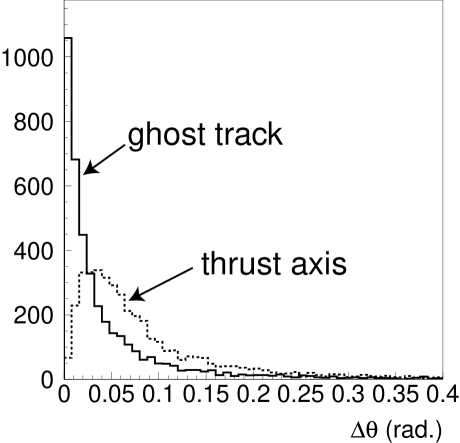
Figure 7: Residual distributions between a true $B$ direction and a ‘ghost’ track/thrust axis. Open histogram indicates the distribution for a ‘ghost’ track and hashed one for a thrust axis. The ‘ghost’ track gives a better $B$ direction estimate than the thrust axis.

The second stage of the algorithm begins by defining a fit probability for a set of tracks to form a vertex with each other and with the ‘ghost’ track (or IP). This probability then measures the likelihood of the set of tracks both belonging to a common vertex and being consistent with the ‘ghost’ track (or IP) and hence forming a part of the $B$ decay chain. These probabilities are determined from the fit $\chi^{2}$ which is in turn determined algebraically from the parameters of the selected tracks and the ‘ghost’ track (or the IP). Fake vertices peak at probability close to 0.

The aim is now to find the most probable track-vertex associations to divide the set of tracks and IP into subsets of reconstructed vertices. Candidate vertices are groups of 1 or more tracks (or IP) considered as the reconstruction develops. For a set of N tracks, there are initially N+1 candidate vertices (N 1-prong secondary vertices and a bare IP). Fit probabilities for all pairs of candidate vertices are calculated together with the ‘ghost’ track. The probabilities of each track associated with the IP are calculated too. The pair of candidate vertices which have the highest probability for fitting in a vertex together is found, and then combined to form a new candidate vertex. This modifies the set of all candidate vertices, and the procedure then repeats with the new set. At each iteration, the number of candidate vertices decreases by one. The iterations continue until the maximum probability is less than 1%. At this point the tracks and IP have been divided into unique subsets by the associations thereby defining topological vertices.

The performance of the ghost track algorithm is quite remarkable. Fig. 8 shows $B$ reconstruction efficiency curves as a function of the $B$ decay length. The ghost track algorithm improves the efficiency along with entire $B$ decay length, particularly at short decay length. The $B$ reconstruction at the short decay length is very important because many $B$ hadrons decay in that region (statistical advantage) and because proper time resolution (essential for $B_{s}$-mixing analysis) is best at short decay lengths.

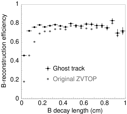
Figure 8: $B$ reconstruction efficiency curves as a function of the $B$ decay length. Black points indicate ghost track algorithm and grey points original topological vertexing algorithm. The ghost track algorithm improves the efficiency along with entire $B$ decay length, in particular short decay length.

The ghost track algorithm improves the $B$ vertex reconstruction purity, too. Here we show the performance of $B_{s}$-charge-dipole-tag purity as an example. Jets or hemispheres in which three vertices are found – the primary (which includes by definition the IP), a secondary and a tertiary – are used for the charge-dipole analysis. The secondary vertex is identified as the $B$ decay vertex and the tertiary as the cascade charm decay, and the charge dipole ($\delta q$) is defined as follows:

$$\delta q=d_{BD}\cdot\mathrm{sign}\left(Q_{D}-Q_{B}\right).$$ (6)

where $d_{BD}$ is the distance between charm and $B$ decay vertices, $Q_{D}$ is the charge of $D$ vertex and $Q_{B}$ the charge of $B$ vertex. Fig. 9 shows the charge-dipole-tag purity versus $B_{s}$ decay length. The ghost track algorithm improves the purity in the entire region, again particularly at the short decay length. The better purity implies that $B-D$ separation is improved, i.e. track attachment for the vertex is improved. It should be mentioned that improving the purity and efficiency of $B$ reconstruction (by requiring the vertices be consistent with a single line of flight), the ghost track algorithm has the additional advantage of allowing the direct reconstruction of 1-prong vertices, including the topology consisting of 1-prong $B$ decay and $D$ decays.

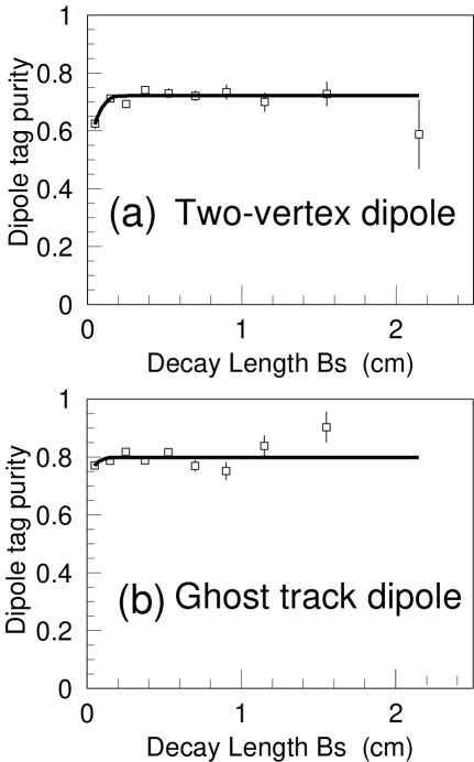
Figure 9: $B_{s}$-charge-dipole-tag purities dependent on the $B$ decay length for (a) original topological vertexing algorithm and (b) the ghost track algorithm. The ghost track algorithm increase purity for the entire region, in particular short decay length.

As the last topic of this section, we show $B$ decay length resolution as evidence of how well the improved track fitter plus the ghost track algorithm work. Fig. 10 illustrates that $B_{s}$-decay-length residual for an earlier dipole algorithm and the improved fitter with the new ghost track algorithm. The improved fitter and the ghost track algorithm reduce the core decay length resolution by $\sim 50\mathrm{\%}$ obtaining a resolution of $107\mu\mathrm{m}$. Even better resolutions are obtained in other analyses. The best one is obtained by the reconstruction of $B_{s}\to D_{s}+X;D_{s}\to\phi+\pi$ mode. In this case, the core resolution is $46\mu\mathrm{m}$. This performance is also unsurpassed by the other experiments.

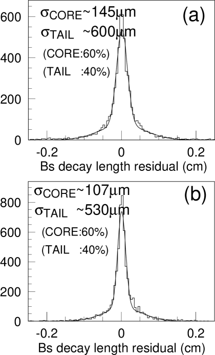
Figure 10: Residual distributions of $B_{s}$ decay length for charge-dipole-tag method. (a) original track fitter plus original topological vertexing algorithm and (b) new track fitter plus the ghost track algorithm. The improved fitter and ghost track algorithm reduces the decay length resolution by $\sim 50\mathrm{\%}$ and obtained resolution of $107\mu\mathrm{m}$.

6 Summary

In this paper, we discussed refinements in alignment, pattern recognition, and track fitting that have significantly improved combined CDC/VXD3 tracking performance. The upgraded tracking performance has resulted in world-record performance. With improvements in topological vertexing technique, it should lead to important physics results including greatly improved sensitivity for $B_{s}$ mixing. The outstanding performance of VXD3 encourages us to aim toward even higher performance goals for vertex detectors at future linear collider detectors [18].

References

- [1] C.J. Damerell, R.L. English, A.R. Gillman, A.L. Lintern, F.J. Wickens and S.J. Watts, IEEE Trans. Nucl. Sci. 33, 51 (1986).
- [2] C.J. Damerell et al., Nucl. Instrum. Meth. A288, 236 (1990).
- [3] C.J. Damerell et al., In *Dallas 1992, Proceedings, High energy physics, vol. 2* 1862-1866.
- [4] D.J. Jackson, Nucl. Instrum. Meth. A388, 247 (1997).
- [5] K. Abe et al. [SLD Collaboration], Phys. Rev. Lett. 80, 660 (1998) hep-ex/9708015.
- [6] K. Abe et al., Nucl. Instrum. Meth. A400, 287 (1997).
- [7] N.B. Sinev et al. [SLD Collaboration], IEEE Trans. Nucl. Sci. 44, 587 (1997).
- [8] J.E. Brau [SLD Collaboration], Nucl. Instrum. Meth. A418, 52 (1998).
- [9] The CCDs were manufactured by the EEV Company, Chelmsford, Essex, UK.
- [10] D.J. Jackson et al., to be submitted to Nucl. Inst. and Meth. A.
- [11] F. James and M. Roos, Comput. Phys. Commun. 10, 343 (1975).
-
[12]
The residual types in Fig. 3
are defined as follows:
-
1.
Doublets: tracks through the overlapping region () of two CCDs on the same ladder. The vectors is fixed at one of the doublet hits and at the furthest-away hit on a different layer. The residual of the second doublet hit to this fixed vector is called the doublet residual.
-
2.
Shingles: tracks through the overlapping shingle region () of two ladders in the same layer. The vector is fixed at the hit on one of the shingle ladders and at the furthest away hit on a different layer. The residual of the hit from the second shingle ladder to the fixed vector is called shingle residual.
-
3.
Triplets: tracks with hits in all three layers. The vector is fixed at the Layer 1 and Layer 3 hits, and the Layer 2 hit residual is called the triplet residual.
-
4.
Pairs: a pair of back-to-back particles. Each vector is given by hits in layers 1 and 3 (layer 2 is ignored for pairs). The residual of the closest approach point between two vectors is called pairs residual.
-
1.
- [13] We use Singular Value Decomposition (SVD) technique in order to solve the equation. A fuller discussion of the mathematical details can be found in G. Golub and C. van Loan, Matrix Computations, (1983) John Hopkins University Press.
- [14] M. Regler and R. Fruhwirth, In *St. Croix 1988, Proceedings, Techniques and concepts of high-energy physics* 407-499. .
- [15] R. Fruhwirth, D. Liko, W. Mitaroff and M. Regler, Presented at 5th Int. Conf. on Instrumentation for Colliding Beam Physics, Novosibirsk, USSR, Mar 15-21, 1990.
- [16] P. Billoir, Nucl. Instr. Meth. A225, 352 (1984).
- [17] D.J. Jackson, reported at the International Europhysics Conference on High Energy Physics, Tampere, Finland, July 15-21, 1999. More detailed discussion can be found in SLAC-PUB-8225.
- [18] P.N. Burrows [LCFI Collaboration], these proceedings hep-ex/9908004.