Partial Wave Analysis of $J/\psi\to\gamma(\pi^{+}\pi^{-}\pi^{+}\pi^{-})$

Abstract

BES data on $J/\psi\to\gamma(\pi^{+}\pi^{-}\pi^{+}\pi^{-})$ have been analyzed into partial waves. We fit with resonances having $J^{PC}=2^{++}$ at 1275 MeV, $0^{++}$ at 1500 MeV, $2^{++}$ at 1565 MeV, $0^{++}$ at 1740 MeV, $2^{++}$ at 1940 MeV and $0^{++}$ at 2104 MeV, plus a broad $0^{-}$ component. The $0^{++}$ resonances decay dominantly to $\sigma\sigma$, while $2^{++}$ resonances in the high mass region decay mainly to $f_{2}(1270)\sigma$ and $\sigma\sigma$; $2^{++}$ resonances from the low mass region decay dominantly to $\rho\rho$.

MARK III and DM2 reported their data on $J/\psi\to\gamma(\pi^{+}\pi^{-}\pi^{+}\pi^{-})$ in 1986 and 1989 respectively [2, 3]. They found that the dominant component of the spectrum below 2 GeV was due to $J/\psi\to\gamma\rho\rho$ with spin-parity $0^{-}$ in the $\rho\rho$ system, where the two $\rho$ appear in a relative P-wave. MARK III claimed a pseudoscalar resonance at $1.55$ GeV/c². This was supported by DM2, and in addition they claimed that structures at $1.80$ and $2.10$ GeV/c² were also $J^{PC}=0^{-+}$.

Later, E760 found three structures in $\eta\eta$ [4] with masses and widths very similar to those observed in $J/\psi\to\gamma\pi^{+}\pi^{-}\pi^{+}\pi^{-}$. However, the quantum numbers $0^{-+}$ are forbidden to $\eta\eta$. Both MARK III and DM2 analyzed their data in terms of $J/\psi\to\gamma\rho\rho\to\gamma\pi^{+}\pi^{-}\pi^{+}\pi^{-}$, but they did not consider $J/\psi\to\gamma\sigma\sigma\to\gamma\pi^{+}\pi^{-}\pi^{+}\pi^{-}$. Here $\sigma$ means the full $\pi-\pi$ S-wave amplitude [5], parametrized up to 1800 MeV. In 1995, Bugg et al. reanalyzed MARK III data [6] and added the $\sigma\sigma$ decay mode to $\rho\rho$. Inclusion of this decay identified two of the peaks as $I=0$ scalar resonances decaying exclusively via $\sigma\sigma$. Those states have masses in the region $M=1500$ and $2100$ MeV/c². An additional scalar state was required at $M=1750$ MeV/c², decaying dominantly to $\sigma\sigma$, but also with significant decays via $\rho\rho$.

We present here an analysis of BES data on $J/\psi\to\gamma\pi^{+}\pi^{-}\pi^{+}\pi^{-}$ into partial waves. In this analysis, the full Monte Carlo simulation of the BES detector is used. This improves on the analysis of Bugg et al., which used only a simplified Monte Carlo simulation, since the full Monte Carlo simulation of the Mark III detector was then no longer available. The full Monte Carlo simulation allows an improved study of the main background channel $J/\psi\to\pi^{0}\pi^{+}\pi^{-}\pi^{+}\pi^{-}$. Results are similar to those of Ref. [6], but with the significant addition that a $2^{+}$ amplitude is required in the high mass region around 2 GeV.

The Beijing Spectrometer(BES) has collected $7.8\times 10^{6}~{}J/\psi$ triggers, used here. Details of the detector are given in Ref. [7]. We describe briefly those detector elements playing a crucial role in the present measurement. Tracking is provided by a 10 superlayer main drift chamber (MDC). Each superlayer contains four layers of sense wires measuring both the position and the ionization energy loss ($d$E$/dx$) of charged particles. The momentum resolution is $\sigma_{P}/P=1.7\%\sqrt{1+P^{2}}$, where $P$ is the momentum of charged particles in GeV/$c$. The resolution of the $d$E$/dx$ measurement is $\sim\pm 9\%$, providing good $\pi/K$ separation and proton identification for momenta up to 600 MeV/c. An array of 48 scintillation counters surrounding the MDC measures the time-of-flight (TOF) of charged particles with a resolution of 330$ps$ for hadrons. Outside the TOF system is an electromagnetic calorimeter made of lead sheets and streamer tubes and having a $z$ positional resolution of 4 cm. The energy resolution scales as $\sigma_{E}/E=22\%/\sqrt{E}$, where $E$ is the energy in GeV. Outside the shower counter is a solenoidal magnet producing a 0.4 Tesla magnetic field.

Candidates for the decay $J/\psi\to\gamma\pi^{+}\pi^{-}\pi^{+}\pi^{-}$ are selected by requiring exactly four charged tracks. Every track must have a good helix fit in the polar angle range $-0.8<\cos\theta<0.8$ and a transverse momentum $>60$ MeV/c. A vertex is required within an interaction region $\pm 20$ cm longitudinally and 2 cm radially. The number of neutral clusters may be up to five, but only one reconstructed $\gamma$ is required in the barrel shower counter. A minimum energy cut of 50 MeV is imposed on the photons. Showers that can be associated with charged tracks are not considered. Four-constraint kinematic fits are performed to the final states $\gamma\gamma 4\pi$, $\gamma 4\pi$ and $4\pi$. The value of $\chi^{2}(\gamma 4\pi)$ is required to be the smallest one. The probability of $\chi^{2}(\gamma 4\pi)$ is required to be larger than $5$%, in order to achieve good resolution and to select a good photon.

Further cuts are as follows. To remove the main background, $J/\psi\to\pi^{0}\pi^{+}\pi^{-}\pi^{+}\pi^{-}$, we required the probability $Prob(\chi^{2}(\gamma 4\pi))$ to be larger than $Prob(\chi^{2}(\gamma\gamma_{miss}4\pi))$, where $\gamma_{miss}$ means this photon is missing. If the two photons in $J/\psi\to\gamma\gamma_{miss}\pi^{+}\pi^{-}\pi^{+}\pi^{-}$ are from a $\pi^{0}$ decay, $Prob(\chi^{2}(\gamma\gamma_{miss}4\pi))$ is required to be $<1$%. Next, $\mid{U_{miss}}\mid=\mid E_{miss}-P_{miss}\mid<0.12$ GeV/c² is required in order to reject events containing more than one photon or containing charged kaons; here, $E_{miss}$ and $P_{miss}$ are, respectively, the missing energy and missing momentum of all charged particles, which are taken to be $\pi^{+}\pi^{-}\pi^{+}\pi^{-}$. The transverse momentum of the $4\pi$ system $P_{t\gamma}^{2}=4\mid{P_{miss}}\mid{{}^{2}}~{}\sin^{2}(\theta_{m\gamma}/2)$ is required to be $<0.005$ (GeV/c)², in order to remove the background $J/\psi\to\pi^{0}\pi^{+}\pi^{-}\pi^{+}\pi^{-}$; here $\theta_{m\gamma}$ is the angle between the missing momentum and the photon direction. Background $J/\psi\to\omega\pi^{+}\pi^{-}$ events are eliminated by the cut $\mid M_{\pi^{+}\pi^{-}\pi^{0}}-M_{\omega}\mid>25$ MeV, in the $\pi^{0}\pi^{+}\pi^{-}\pi^{+}\pi^{-}$ hypothesis with only one photon detected and the $\pi^{0}$ associated to the missing momentum. To remove the small background due to $J/\psi\to\gamma K_{s}^{0}K_{s}^{0}$ events, a double cut on the two $\pi^{+}\pi^{-}$ invariant masses is performed, $\mid M_{\pi^{+}\pi^{-}}-M_{K_{s}^{0}}\mid>25$ MeV. The BES data show a small signal due to $f_{1}(1285)$; this is not important for our conclusion and not of concern in this analysis, so, in order to remove it, an additional cut is applied to discard events within the mass region between $1.24$ and $1.32$ GeV/c².

The effects of the various selection cuts on the data is simulated with a full Monte Carlo of the BES detector; 200,000 Monte Carlo events are successfully fitted to $J/\psi\to\gamma(\pi^{+}\pi^{-}\pi^{+}\pi^{-})$ with $4\pi$ mass below 2.4 GeV; all background reactions are similarly fitted to this channel. The estimated background is 31%, purely from $J/\psi\to\pi^{0}(\pi^{+}\pi^{-}\pi^{+}\pi^{-})$. We have included this background in the amplitude analysis; it lies very close to phase space of $J/\psi\to\gamma(\pi^{+}\pi^{-}\pi^{+}\pi^{-})$ and has only a small effect on the fit. It includes a small signal (visible in Fig. 3(c) and (d) below) for $a_{2}(1320)\to\rho\pi$, originating from $J/\psi\to a_{2}\rho$. When this $a_{2}(1320)$ signal is combined with a fourth pion, it does not correlate with any peak in the $4\pi$ mass spectrum. Otherwise, the $4\pi$ and $3\pi$ mass distributions in the background lie very close to phase space and are parametrised by phase space distributions.

Fig. 1 shows the $2\pi$ invariant mass distribution after acceptance cuts. The acceptance from the Monte Carlo simulation is included into the maximum likelihood fit. Signals are seen due to $\rho$ (or $\sigma$) and $f_{2}(1270)$. The $\sigma$ contains two components, one very broad and the other with a peak near the $\rho$ and somewhat wider than the $\rho$. It cannot be reliably separated from the $\rho$ as a peak. The two are distinguished by their quite different angular dependence. They are quite easy to distinguish in the fit, but this is not easily displayed graphically, because of the two combinations. The lowest peak of Fig. 1(b) is due to conversion electrons, and has been cut out in the fit. The $4\pi$ invariant mass distribution for $J/\psi\to\gamma\pi^{+}\pi^{-}\pi^{+}\pi^{-}$ is shown with error bars in Fig. 2; the amplitude analysis resolves structures from $1.50$ to $2.30$ GeV/c². The dark dashed histogram of Fig. 2 shows the $4\pi$ mass spectrum of $J/\psi\to\gamma f_{2}(1270)\sigma$, which rises strongly above 1750 MeV. For our final fit, we use 1988 events below a $4\pi$ mass of 2.4 GeV.

We have carried out a partial wave analysis using amplitudes constructed from Lorentz-invariant combinations of the 4-vectors and the photon polarization for $J/\psi$ initial states with helicity $\pm 1$. Cross sections are summed over photon polarizations. The relative magnitudes and phases of the amplitudes are determined by a maximum likelihood fit. We use $\ell$ to denote the orbital angular momentum between the photon from $J/\psi$ decay and the resonance in the production process; we use $L$ to denote the orbital angular momentum in the decay of the resonance to final states $\rho\rho$, $\sigma\sigma$ and $f_{2}(1270)\sigma$, with $L$ restricted $\leq 2$. Because production is via an electromagnetic transition, the same phase is used for amplitudes with different $\ell$ but otherwise the same final state.

We now discuss resonances and possible decay modes which have been included in the fit. Spin-parity assignments up to $J=4$ have been tried. We have tried to include $\pi-\pi(1300)$ or $\pi-a_{1}(1260)$ decay modes for $0^{+}$ resonance. There are two decay modes of $\pi(1300)$ and $a_{1}(1260)$: $\rho\pi$ and $\sigma\pi$. From the PDG [8], $\pi(1300)$ and $a_{1}(1260)$ decay mainly to $\rho\pi$. When putting this constraint into the fit, we found the contributions of the $\pi-\pi(1300)$ and $\pi-a_{1}(1260)$ decay modes are negligible. The resonances and decay modes which make significant improvements in log likelihood are listed in Table I. Amplitudes are constructed in terms of the combined spin $S$ of the decay photon and the $J/\psi$ system.

The dominant component in the fit is $0^{-}$. We find that this may be parametrized in two alternative ways. The one used for the fit reported here is a simple Breit-Wigner amplitude of mass 1440 MeV and width 225 MeV. It is much wider than $\eta(1440)$ and is therefore not to be identified with that state. The rapidly increasing phase space for decays to $\rho\rho$ with $L=1$ results in a very broad $0^{-}$ signal, illustrated below in Fig. 4(a). An alternative more complicated parametrization is given in a recent coupled channel analysis of many $J/\psi$ decay modes [9]; it gives results almost indistinguishable from those presented here.

The width of $f_{2}(1270)$ cannot be fitted with any precision. Statistics of data in the $f_{2}(1270)$ mass region are very low because the $f_{1}(1285)$ has been removed by a cut in this mass region. Hence the mass and width of the $f_{2}(1270)$ are constrained to the PDG value [8]. Some $2^{+}$ component is definitely required in the mass range 1500–1700 MeV, as is illustrated below in Fig. 4(c). This may be attributed to $f_{2}(1565)$, which sits at the $\rho\rho$ and $\omega\omega$ threshold and can decay into $4\pi$. In the final fit, the mass of $f_{2}(1565)$ has been fixed at 1565 MeV, which is well determined by data from other sources [10] [11] [12]. The possible cause of our optimum mass for $f_{2}(1565)$ lying at 1505 MeV may be crosstalk between the two neighboring resonances ($f_{0}(1500)$ and $f_{2}(1565)$). Once the masses and widths are fixed, both contributions are well determined.

Comparisons with data are shown in Fig. 3 summed from $M(4\pi)=1.0$ to 2.4 GeV for $M_{\pi^{+}\pi^{-}\pi^{+}\pi^{-}}$, $M_{\pi^{+}\pi^{-}}$, $M_{3\pi}$, $M_{\rho\pi}$, $\cos\theta_{\pi^{+}}$; here $\theta_{\pi^{+}}$ is the angle of $\pi^{+}$ with respect to the $\pi^{+}\pi^{-}$ pair in their rest frame, and $\chi$ is the azimuthal angle between the planes of $\pi^{+}\pi^{-}$ pairs in the rest frame of the resonance X. The contributions of the various components in this fit are shown in Fig. 4 and Fig. 5; crosses are data and histograms the fit.

From Fig. 5, it can be seen that $2^{+}$ resonances in the high mass region decay mainly via $f_{2}(1270)\sigma$ and $\sigma\sigma$; the $2^{+}$ resonances in the low mass region decay mainly via $\rho\rho$. The peak of $f_{2}(1565)$ appears at $\sim 1580$ MeV because of the rapidly increasing phase space for its $4\pi$ decay. The $2^{+}$ signals at about 1580 MeV with L=0 and L=2 are both larger than the combined signals in Figure 4; the reason for this is destructive interference between L=0 and L=2.

Branching fractions are given in Table II. The branching fraction for $M_{4\pi}<3.0$ GeV/c² is $Br(J/\psi\to\gamma\pi^{+}\pi^{-}\pi^{+}\pi^{-})=(3.8\pm 0.3\pm 1.3)\times 10^{-3}.$ The first error is statistical and the second systematic.

In order to check whether the final full fit is the best solution for BES data, four tests are performed.

The first test is to check the significance level of each resonance. The $0^{-}$ contribution of Fig. 4 is definitely required; without it, log likelihood gets worse by 293.1. Table III summarizes the changes in log likelihood when each resonance of the fit is dropped and remaining contributions are re-optimized. It indicates that the $f_{2}(1270)$, $f_{0}(1500)$, $f_{2}(1565)$, $f_{0}(1740)$, $f_{2}(1950)$ and $f_{0}(2100)$ should be included.

The second test is to check the $J^{P}$ assignment of each resonance. Table IV shows the effect of substituting alternative $J^{P}$ assignments for each resonance. It can be seen that making an alternative $J^{P}$ assignment for each resonance is rejected clearly.

The third test is to scan for an additional structure. Scanning an additional structure in $0^{-}$, $0^{+}$, $2^{+}$, or $4^{+}$ with 2, 4, 6 and 4 more free parameters respectively indicates no further distinctive structures. The BES data on $J/\psi\to\gamma K^{+}K^{-}$ [13] show two possible resonance in the 1.7 GeV region: a scalar with mass 1781 MeV, a tensor 1696 MeV. We have therefore tried adding to the fit a tensor resonance in this mass region. We have found no significant production of spin 2 is observed in the $\gamma\pi^{+}\pi^{-}\pi^{+}\pi^{-}$ channel.

The fourth test is to fit the data in slices of mass. The data are fitted in each of 10 mass bins 100 MeV wide from 1350 to 2350 MeV. The comparisons of the full fit and the slice fit are plotted in Fig. 6. The solid line presents the full fit results, while the dot stands for the slice analysis results. They are in fair agreement with each other. The slice analysis confirms strongly the presence of a tensor component in the mass region around 2000 MeV.

The results are summarized as follows: The $0^{++}$ resonances decay dominantly to $\sigma\sigma$, while the $2^{++}$ resonances in the low mass region decay dominantly to $\rho\rho$, and those in the high mass region decay to $f_{2}(1270)\sigma$, $\sigma\sigma$.

The $f_{0}(1500)$ and $f_{0}(1740)$ are produced significantly in $J/\psi\to\gamma\pi^{+}\pi^{-}\pi^{+}\pi^{-}$; according to the criteria of determining the gluonic content of resonance in radiative $J/\psi$ decays proposed by Close et al.[14], they may therefore contain significant glueball components.

The BES results are approximately consistent with the results from the earlier re-analysis of MARK III data [4]. But the BES data favour more $2^{+}$ in the high mass region. A possible cause of this difference is that a better background function for BES data is available and a full Monte Carlo simulation is employed in BES analysis. An important conclusion is that a broad $2^{+}$ resonance $f_{2}(1950)$ is needed around 2 GeV. This is where the $2^{+}$ glueball may be expected, and $J/\psi$ radiative decays are supposed to be one of the best places to search for it. The $f_{2}(1950)$ was first observed by the WA91 group [15] and subsequently confirmed by the WA102 group in their $4\pi$ mass spectrum [16]; this agrees with our observation.

The BES group thanks the staff of IHEP for technical support in running the experiment. This work is supported in part by China Postdoctoral Science Foundation and National Natural Science Foundation of China under contract Nos. 19991480, 19825116 and 19605007; and by the Chinese Academy of Sciences under contract No. KJ 95T–03(IHEP). We also acknowledge financial support from the Royal Society for collaboration between Chinese and UK groups.

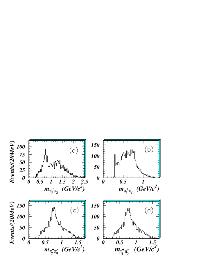
FIG. 1.: The $2\pi$ mass spectrum of $J/\psi\to\gamma\pi^{+}\pi^{-}\pi^{+}\pi^{-}$, taking $P(\pi_{1}^{+})>P(\pi_{3}^{+})$ and $P(\pi_{2}^{-})>P(\pi_{4}^{-})$.

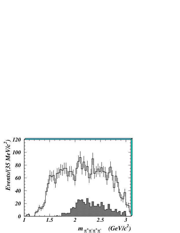
FIG. 2.: The $4\pi$ mass spectrum of $J/\psi\to\gamma\pi^{+}\pi^{-}\pi^{+}\pi^{-}$; the dark shaded histogram is the $4\pi$ mass spectrum of $J/\psi\to\gamma f_{2}(1270)\sigma$

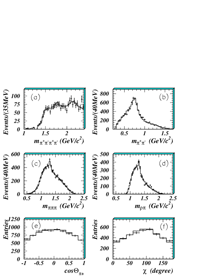
FIG. 3.: The comparison between data and final full fit.

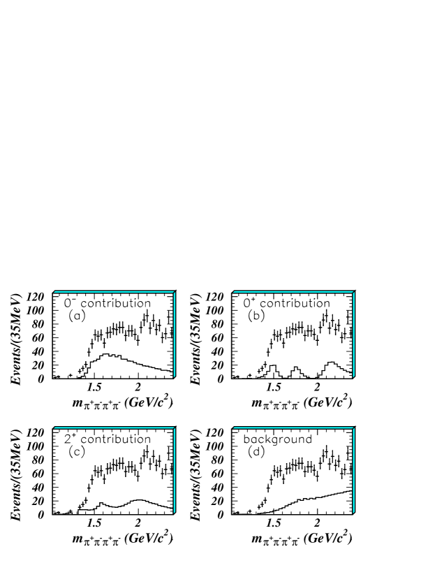
FIG. 4.: component contribution.

FIG. 5.: tensor component contribution.

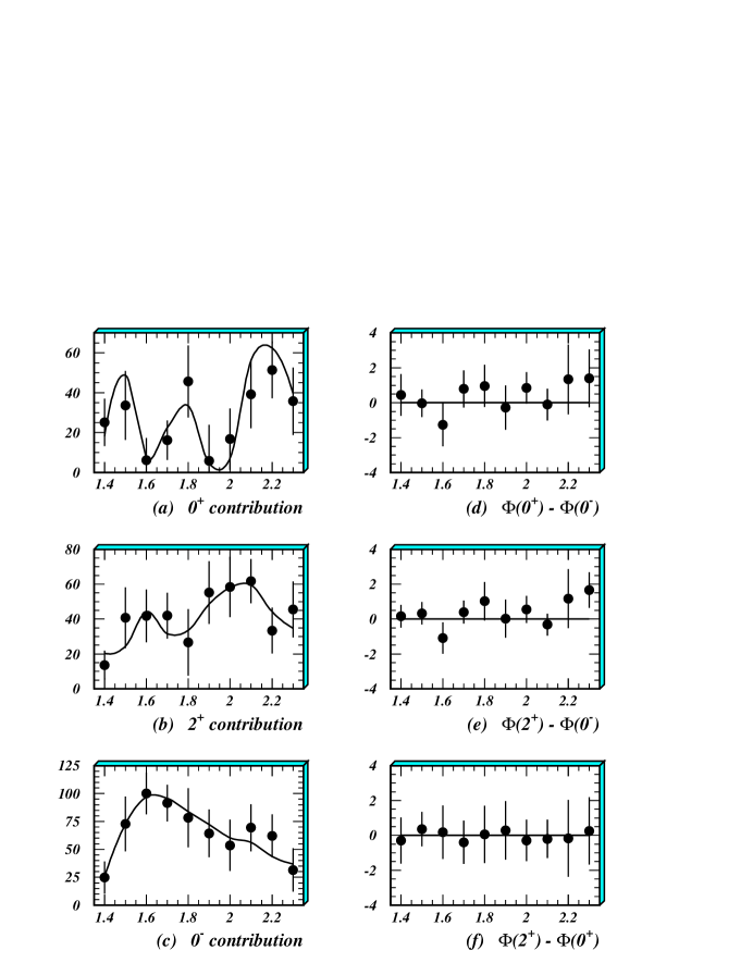
FIG. 6.: Numbers of events in 100 MeV slices of $M(4\pi)$ (data point) from (a) $0^{+}$, (b) $2^{+}$ and (c) $0^{-}$ and the full fit (curves); the discrepancy in phase difference (d) $\phi(0^{+})-\phi(0^{-})$, (e) $\phi(2^{+})-\phi(0^{-})$ and (f) $\phi(2^{+})-\phi(0^{+})$ between the data and fit(radians); the value plotted is that for each slice minus the value from the fit.

TABLE I.: Resonances fitted to the BES data and decay modes used in the final fit.

		Measured		Used in final fit		decays	$\ell$ or ${}^{2S+1}\ell_{2}~{}$
$J^{P}$	Resonance	Mass	$\Gamma$	Mass	$\Gamma$
		(MeV)	(MeV)	(MeV)	(MeV)
$2^{+}$	$f_{2}(1270)$	$1280^{+35}_{-20}$		1275	185	$\rho\rho$	${}^{1}D_{2}~{}^{3}D_{2}$
$0^{-}$		$1440^{+20}_{-20}$	$225^{+25}_{-20}$	1440	225	$\rho\rho$	$\ell=1~{}~{}~{}~{}~{}~{}~{}~{}~{}~{}$
$0^{+}$	$f_{0}(1500)$	$1505^{+15}_{-20}$	$140^{+40}_{-30}$	1500	112	$\sigma\sigma$	$\ell=0~{}~{}~{}~{}~{}~{}~{}~{}~{}~{}$
$2^{+}$	$f_{2}(1565)$	$1505^{+60}_{-20}$	$135^{+30}_{-25}$	1565	131	$\rho\rho$	${}^{5}S_{2}~{}~{}~{}~{}~{}~{}~{}~{}~{}~{}~{}~{}$
$0^{+}$	$f_{0}(1740)$	$1740^{+30}_{-25}$	$120^{+50}_{-40}$	1740	120	$\sigma\sigma$	$\ell=0~{}~{}~{}~{}~{}~{}~{}~{}~{}~{}$
$2^{+}$	$f_{2}(1950)$	$1940^{+50}_{-50}$	$380^{+120}_{-~{}90}$	1940	380	$f_{2}(1270)\sigma$	${}^{5}S_{2}~{}~{}~{}~{}~{}~{}~{}~{}~{}~{}~{}~{}$
						$\sigma\sigma$	${}^{1}D_{2}~{}^{3}D_{2}$
$0^{+}$	$f_{0}(2100)$	$2090^{+30}_{-30}$	$330^{+100}_{-100}$	2104	215	$\sigma\sigma$	$\ell=0~{}~{}~{}~{}~{}~{}~{}~{}~{}~{}$

TABLE II.: Branching ratios for various final states in $J/\psi$ decays, integrated up to $M(4\pi)=2400$ MeV. The first error is statistical and the second systematic.

Process	Branching ratios
$Br(J/\psi\to\gamma f_{2}(1270))\times Br(f_{2}(1270)\to\pi^{+}\pi^{-}\pi^{+}\pi^{-})$	$(1.8\pm 0.2\pm 0.6)\times 10^{-4}$
$Br(J/\psi\to\gamma 0^{-})~{}~{}~{}~{}~{}~{}~{}~{}\times Br(0^{-}\to\pi^{+}\pi^{-}\pi^{+}\pi^{-})$	$(1.2\pm 0.1\pm 0.4)\times 10^{-3}$
$Br(J/\psi\to\gamma f_{0}(1500))\times Br(f_{0}(1500)\to\pi^{+}\pi^{-}\pi^{+}\pi^{-})$	$(3.1\pm 0.2\pm 1.1)\times 10^{-4}$
$Br(J/\psi\to\gamma f_{2}(1565))\times Br(f_{2}(1565)\to\pi^{+}\pi^{-}\pi^{+}\pi^{-})$	$(3.2\pm 0.2\pm 1.1)\times 10^{-4}$
$Br(J/\psi\to\gamma f_{0}(1740))\times Br(f_{0}(1740)\to\pi^{+}\pi^{-}\pi^{+}\pi^{-})$	$(3.1\pm 0.2\pm 1.1)\times 10^{-4}$
$Br(J/\psi\to\gamma f_{2}(1950))\times Br(f_{2}(1950)\to\pi^{+}\pi^{-}\pi^{+}\pi^{-})$	$(5.5\pm 0.3\pm 1.9)\times 10^{-4}$
$Br(J/\psi\to\gamma f_{0}(2100))\times Br(f_{0}(2100)\to\pi^{+}\pi^{-}\pi^{+}\pi^{-})$	$(5.1\pm 0.3\pm 1.8)\times 10^{-4}$

TABLE III.: Changes $\Delta S$ in log likelihood function S when various components of the fit are dropped and remaining contributions are re-optimized.

$J^{P}$	Resonance	$\Delta S$	Freedom	Significance level
$2^{+}$	$f_{2}(1270)$	+18.67	5	5.0$\sigma$
$0^{+}$	$f_{0}(1500)$	+21.79	4	$>$6.0$\sigma$
$2^{+}$	$f_{2}(1565)$	+16.32	4	4.8$\sigma$
$0^{+}$	$f_{0}(1740)$	+17.73	4	5.1$\sigma$
$2^{+}$	$f_{2}(1950)$	+37.30	7	$>$6.0$\sigma$
$0^{+}$	$f_{0}(2100)$	+23.58	4	$>$6.0$\sigma$

TABLE IV.: Changes $\Delta S$ in log likelihood function when various components are assigned a different $J^{P}$ and all contributions are re-optimized.

$J^{P}$	Resonance	$0^{-}$	$0^{+}$	$2^{+}$	$4^{+}$
$2^{+}$	$f_{2}(1270)$	+15.1	+13.2		+16.5
$0^{+}$	$f_{0}(1500)$	+18.0		+9.6	+17.2
$2^{+}$	$f_{2}(1565)$	+15.5	+16.0		+11.0
$0^{+}$	$f_{0}(1740)$	+16.8		+11.6	+15.7
$2^{+}$	$f_{2}(1950)$	+36.4	+28.2		+31.6
$0^{+}$	$f_{0}(2100)$	+13.2		+10.0	+18.1

REFERENCES

- [1] Data analyzed were taken prior to the participation of U.S. members of the BES Collaboration.
- [2] R.M. Baltrusaitis et al., Phys. Rev. D 33 (1986) 1222.
- [3] D. Bisello et al., Phys. Rev. D 39 (1989) 701.
- [4] T.A. Armstrong et al., Phys. Lett. B 307 (1993) 394.
- [5] B.S. Zou and D.V. Bugg, Phys. Rev. D 48 (1993) 3948.
- [6] D.V. Bugg et al., Phys. Lett. B 353 (1995) 378.
- [7] BES Collaboration, Nucl. Instr. Methods, A 344 (1994) 319.
- [8] Particle Data Group, Euro. Phys. J. C 3 (1998) 1.
- [9] D.V. Bugg, L.Y. Dong and B.S. Zou, Phys. Lett. B 458 (1999) 511.
- [10] B. May et al., Phys. Lett. B 225 (1989) 450.
- [11] A. Abele et al., Nucl. Phys. A 609 (1996) 562.
- [12] C.A. Baker et al., Phys. Lett. B (to be published).
- [13] J.Z. Bai et al., Phys. Rev. Lett., 77 (1996) 3959.
- [14] F.E. Close et al., Phys. Rev. D 55 (1997) 5749.
- [15] F. Antinori et al., Phys. Lett. B 353 (1995) 589.
- [16] D. Barberis et al., Phys. Lett. B 397 (1997) 339.