$\psi(2S)\rightarrow\pi^{+}\pi^{-}J/\psi$ Decay Distributions [2]

Abstract

Using a sample of 3.8 M $\psi(2S)$ events accumulated with the BES detector, the process $\psi(2S)\rightarrow\pi^{+}\pi^{-}J/\psi$ is studied. The angular distributions are compared with the general decay amplitude analysis of Cahn. We find that the dipion system requires some D-wave, as well as S-wave. On the other hand, the $J/\psi$ - $(\pi^{+}\pi^{-})$ relative angular momentum is consistent with being pure S-wave. The decay distributions have been fit to heavy quarkonium models, including the Novikov-Shifman model. This model, which is written in terms of the parameter $\kappa$, predicts that D-wave should be present. We determine $\kappa=0.183\pm 0.002\pm 0.003$ based on the joint $m_{\pi\pi}$ - $\cos\theta_{\pi}^{*}$ distribution. The fraction of D-wave as a function of $m_{\pi\pi}$ is found to decrease with increasing $m_{\pi\pi}$, in agreement with the model. We have also fit the Mannel-Yan model, which is another model that allows D-wave.

I Introduction

Transitions between bound $c\bar{c}$ states as well as between $b\bar{b}$ states provide an excellent laboratory for studying heavy quark-antiquark dynamics at short distances. Here we study the process $\psi(2S)\rightarrow\pi^{+}\pi^{-}J/\psi$, which is the largest decay mode of the $\psi(2S)$ [3]. The dynamics of this process can be investigated using very clean exclusive $\psi(2S)\rightarrow\pi^{+}\pi^{-}J/\psi$, $J/\psi\rightarrow l^{+}l^{-}$ events, where $l$ signifies either $e$ or $\mu$.

Early investigation of this decay by Mark I [4] found that the $\pi^{+}\pi^{-}$ mass distribution was strongly peaked towards higher mass values, in contrast to what was expected from phase space. Further, angular distributions strongly favored S-wave production of $\pi\pi J/\psi$, as well as an S-wave decay of the dipion system.

The challenge of describing the mass spectrum attracted considerable theoretical interest. Brown and Cahn [5] and Voloshin [6] used chiral symmetry arguments and partially conserved axial currents (PCAC) to derive a matrix element. Assuming chiral symmetry breaking to be small, Brown and Cahn showed the decay amplitude for this process involves three parameters, which are the coefficients of three different momentum dependent terms. If two of the parameters vanish, then the remaining term would give a peak at high invariant mass along with the isotropic S-wave behavior. In a more general analysis, Cahn [7] calculated the angular distributions in terms of partial wave amplitudes diagonal in orbital and spin angular momentum.

These transitions are thought to occur in a two step process by the emission of two gluons followed by hadronization to pion pairs, as indicated in Fig. 1. Because of the small mass difference involved, the gluons are soft and can not be handled by perturbative QCD. However, Gottfried [8] suggested that the gluon emission can be described by a multipole expansion with the gluon fields being expanded in a multipole series similar to electromagnetic transitions. Including the leading chromo-electric $E1$$E1$ transition, T. M. Yan [9] determined that one of the terms that Brown and Cahn took to be zero should have a small but nonzero value. Voloshin and Zakharov [10] and later, in a revised analysis, Novikov and Shifman [11] worked out the second step, the pion hadronization matrix element using current algebra, PCAC, and gauge invariance. They were able to derive an amplitude for this process from “first principles.” Interestingly, Ref. [11] predicts that while the decay should be predominantly S-wave, a small amount of D-wave should be present in the dipion system.

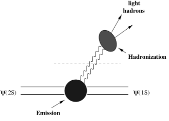
FIG. 1.: Diagram of $\psi(2S)\rightarrow\pi^{+}\pi^{-}J/\psi$ decay process, showing it as a two step process with the emission of two gluons followed by hadronization to pion pairs.

All models predict the spectrum to peak at high mass as it does in $\psi(2S)\rightarrow\pi^{+}\pi^{-}J/\psi$ and $\Upsilon(2S)\rightarrow\pi\pi\Upsilon(1S)$. However, $\Upsilon(3S)\rightarrow\pi^{+}\pi^{-}\Upsilon(1S)$ [12] has a peak at low mass, as well as a peak at high mass, that disagrees with these predictions. See Ref. [12] for a list of theory papers that attempt to deal with this problem.

In this paper, we will study the decay distributions of the $\psi(2S)\rightarrow\pi^{+}\pi^{-}J/\psi$ process and use them to test models. The events come from a data sample of $3.8\times 10^{6}$ $\psi(2S)$ decays taken with the BES detector.

II The BES detector

The Beijing Spectrometer, BES, is a conventional cylindrical magnetic detector that is coaxial with the BEPC colliding $e^{+}e^{-}$ beams. It is described in detail in Ref. [13]. A four-layer central drift chamber (CDC) surrounding the beampipe provides trigger information. Outside the CDC, the forty-layer main drift chamber (MDC) provides tracking and energy-loss ($dE/dx$) information on charged tracks over $85\%$ of the total solid angle. The momentum resolution is $\sigma_{p}/p=1.7\%\sqrt{1+p^{2}}$ ($p$ in GeV/c), and the $dE/dx$ resolution for hadron tracks for this data sample is $\sim 9\%$. An array of 48 scintillation counters surrounding the MDC provides measurements of the time-of-flight (TOF) of charged tracks with a resolution of $\sim 450$ ps for hadrons. Outside the TOF system, a 12 radiation length lead-gas barrel shower counter (BSC), operating in self-quenching streamer mode, measures the energies of electrons and photons over 80% of the total solid angle. The energy resolution is $\sigma_{E}/E=22\%/\sqrt{E}$ ($E$ in GeV). Surrounding the BSC is a solenoidal magnet that provides a 0.4 Tesla magnetic field in the central tracking region of the detector. Three double layers of proportional chambers instrument the magnet flux return (MUID) and are used to identify muons of momentum greater than 0.5 GeV/c.

III Event Selection

In order to study the process $\psi(2S)\rightarrow\pi^{+}\pi^{-}J/\psi$, we use the very clean $\psi(2S)\rightarrow\pi^{+}\pi^{-}J/\psi$, $J/\psi\rightarrow l^{+}l^{-}$ sample. The initial event selection is the same as in Ref. [14]. We require four tracks total with the sum of the charge equal zero.

A Pion Selection

We require a pair of oppositely charged candidate pion tracks with good helix fits that satisfy:

1. $|\cos\theta_{\pi}|<0.75$. Here $\theta_{\pi}$ is the polar angle of the $\pi$ in the laboratory system.

2. $p_{\pi}<0.5$ GeV/c, where $p_{\pi}$ is the pion momentum.

3. $pxy_{\pi}>0.1$ GeV/c, where $pxy_{\pi}$ is the momentum of the pion transverse to the beam direction. This removes tracks that circle in the Main Drift Chamber.

4. $\cos\theta_{\pi\pi}<0.9,$ where $\theta_{\pi\pi}$ is the laboratory angle between the $\pi^{+}$ and $\pi^{-}$. This cut is used to eliminate contamination from misidentified $e^{+}e^{-}$ pairs from $\gamma$ conversions.

5. $3.0<m_{recoil}<3.2$ GeV/c², where $m_{recoil}$ is the mass recoiling against the dipion system.

6. $|\chi^{dE/dx}_{\pi}|<3.0$. $\chi^{dE/dx}_{\pi}=\frac{(dE/dx)_{meas}-(dE/dx)_{exp}}{\sigma}$ where $(dE/dx)_{meas}$ and $(dE/dx)_{exp}$ are the measured and expected $dE/dx$ energy losses for pions, respectively, and $\sigma$ is the experimental $dE/dx$ resolution.

B Lepton Selection

The lepton tracks must satisfy:

1. $0.5<p_{l}<2.5$ GeV/c. Here $p_{l}$ is the three-momentum of the candidate lepton track.

2. $|\cos\theta_{e}|<0.75$, $|\cos\theta_{\mu}|<0.60$. Here $\theta_{e}$ and $\theta_{\mu}$ are the laboratory polar angles of the electron and muon, respectively. This cut ensures that electrons are contained in the $BSC$ and muons in the MUID system.

3. $\cos\theta_{l^{+}l^{-}}^{cm}<-0.975$. This is the cosine of the angle between the two leptons in the $J/\psi$ CM, where the leptons are nearly back-to-back.

4. $p_{l^{+}}$ or $p_{l^{-}}>1.3$ GeV/c or $p_{l^{+}}+p_{l^{-}}>2.4$ GeV/c. This cut selects events consistent with $J/\psi$ decay, while rejecting background.

5. For $e^{+}e^{-}$ candidate pairs: $SCE_{+}$ and $SCE_{-}>0.6$ GeV/c, where $SCE$ is the energy deposited in the BSC, or, if one of the tracks goes through a BSC rib or has $P_{l}<0.8$ GeV/c, the $dE/dx$ information of both tracks in the MDC must be consistent with that expected for electrons. The rib region of the BSC is not used because the Monte Carlo does not model the energy deposition well in this region.

6. For $\mu^{+}\mu^{-}$ pair candidates at least one track must have $N^{hit}>1$, where $N^{hit}$ is the number of MUID layers with matched hits and ranges from 0 to 3. If only one track is identified in this fashion, then the invariant mass of the $\mu\mu$ pair must also be within 250 MeV/c² of the $J/\psi$ mass.

C Additional Criteria

Fig. 2a shows the $m_{recoil}$ distribution using the cuts defined above. The shoulder above the $J/\psi$ peak is caused by low energy pions that undergo $\pi\rightarrow\mu\nu$ decay. We impose additional selection criteria in order to reduce the amount of mismeasured events from these and from other events where the $J/\psi$ undergoes final state radiation or where electrons radiate much of their energy. These cuts are necessary for comparisons with theoretical models.

1. The $\pi$’s must be consistent with coming from the interaction point.

2. $3.07<m_{recoil}<3.12$ GeV/c².

3. $|m_{l^{+}l^{-}}-m_{J/\psi}|<0.25$ GeV/c², where $m_{l^{+}l^{-}}$ is the invariant mass of the two leptons.

Fig. 2b shows the $m_{recoil}$ distribution using all cuts except the additional $m_{recoil}$ cut (additional cut number 2). A total of 22.8 K events remains after all cuts, and the background remaining is estimated to be less than 0.3 %.

FIG. 2.: (a) Number of events versus $m_{recoil}$, the mass recoiling against the two $\pi$’s, for $\psi(2S)\rightarrow\pi^{+}\pi^{-}J/\psi,J/\psi\rightarrow l^{+}l^{-}$ events where only the initial selection criteria (see text) are used. (b) Number of events versus $m_{recoil}$ where all criteria are used except for the final $m_{recoil}$ cut.

IV Monte Carlo

The process is considered to take place via sequential 2-body decays: $\psi(2S)\rightarrow X+J/\psi$, $X\rightarrow\pi^{+}\pi^{-}$, and $J/\psi\rightarrow l^{+}l^{-}$. The Monte Carlo program assumes:

1. The mass of the dipion system is empirically given by:

   $\displaystyle\frac{d\sigma}{dm_{\pi\pi}}\propto({\rm phase}\,{\rm space})\times(m_{\pi\pi}^{2}-4m_{\pi}^{2})^{2}$

2. The orbital angular momentum between the dipion system and the $J/\psi$ and between the $\pi$’s in the $\pi^{+}\pi^{-}$ system is 0.

3. The X and the $J/\psi$ are uniformly distributed in $\cos\theta$ in the incoming $e^{+}e^{-}$ rest frame, which is the same as the laboratory frame.

4. The $\pi$’s are uniformly distributed in $\cos\theta_{\pi}^{*}$, where $\theta_{\pi}^{*}$ is the angle between the $J/\psi$ direction and the $\pi^{+}$ in the X rest frame.

5. Leptons have a $1+\cos^{2}\theta_{l}^{*}$ distribution, where $\theta_{l}^{*}$ is the angle between the beam direction and the positive lepton in the $J/\psi$ rest frame.

6. The $J/\psi$ decay has an order $\alpha^{3}$ final state radiative correction in the rest frame of the $J/\psi$.

A total of 570,000 Monte Carlo events are generated each for the $\psi(2S)\rightarrow\pi^{+}\pi^{-}J/\psi$, $J/\psi\rightarrow e^{+}e^{-}$ and $\psi(2S)\rightarrow\pi^{+}\pi^{-}J/\psi$, $J/\psi\rightarrow\mu^{+}\mu^{-}$ samples.

In order to compare with theoretical models, the experimental distributions must be corrected for detection efficiency. To determine this correction, Monte Carlo data is run through the same analysis program as the data. A bin-by-bin efficiency correction is then determined for each distribution of interest using the generated and detected Monte Carlo data. This efficiency is then used to correct each bin of the data distributions [15].

A comparison of some distributions with the Monte Carlo distributions is shown in Fig. 3. Fig. 3a indicates that the $m_{\pi\pi}$ distribution agrees qualitatively with the assumed empirical distribution [16]. Fig. 3b indicates agreement with the assumed $1+\cos^{2}\theta_{l}^{*}$ distribution for leptons in $\psi(2S)\rightarrow\pi^{+}\pi^{-}J/\psi$, $J/\psi\rightarrow l^{+}l^{-}$ events. The flat distribution in Fig. 3c is related to the assumption that the relative angular momentum between the dipion system and the $J/\psi$ is zero. However, in Fig. 3d, which is the $\cos\theta_{\pi^{+}}^{*}$ distribution, we find a disagreement with the Monte Carlo data, indicating that the relative angular momentum of the two $\pi$’s is inconsistent with being pure S-wave.

FIG. 3.: Various distributions (corrected for detection efficiency) for $\psi(2S)\rightarrow\pi^{+}\pi^{-}J/\psi$, $J/\psi\rightarrow l^{+}l^{-}$ decays. (a) $m_{\pi^{+}\pi^{-}}$ distribution. The distribution is in reasonable agreement with the assumed empirical distribution. (b) $\cos\theta_{l}^{*}$ distribution. The assumed distribution is a $1+\cos^{2}\theta_{l}^{*}$ distribution. This angle is the angle between the beam direction and the $l^{+}$ in the rest frame of the $J/\psi$. (c) $\cos\theta_{X}$ distribution. This is the cosine of the angle of the dipion system with respect to the $e^{+}e^{-}$ direction in the incoming $e^{+}e^{-}$ CM system. The distribution for Monte Carlo data is flat because of the S-wave assumption for the relative angular momentum of the dipion system and the $J/\psi$. (d) $\cos\theta_{\pi^{+}}^{*}$ distribution. This is the cosine of the angle of the $\pi^{+}$ with respect to the $J/\psi$ direction in the dipion rest frame. The Monte Carlo distribution is flat because of the assumption that the relative angular momentum of the $\pi$’s is S-wave. The data agree well with the Monte Carlo except in (d).

Fig. 4 shows the $\phi$ angle distributions for the $l^{+}$ in the lab; the $J/\psi$ in the lab; the $\pi^{+}$ in the rest frame of the dipion system, $\phi_{\pi^{+}}$; and the angle between the normals to the $\mu\mu$ plane and the $\pi\pi$ plane.

$\displaystyle\phi_{\pi^{+}}=\arctan\left[\frac{(\widehat{(\widehat{\hat{X}\times\hat{z})}\times\hat{X})}\cdot\widehat{p_{\pi^{+}}}}{\widehat{(\hat{X}\times\hat{z})}\cdot\widehat{p_{\pi^{+}}}}\right]$All distributions are uniform in angle, consistent with the Monte Carlo distributions.

Since Fig. 3d indicates an inadequacy with the Monte Carlo, it is necessary to correct our bin-by-bin efficiency determination in our following studies. We use the Novikov-Shifman model (discussed below), which gives a reasonable approximation to the data, to determine a weighting for Monte Carlo events so that the proper efficiency is determined as a function of $\cos\theta_{\pi}^{*}$ and $m_{\pi\pi}$.

FIG. 4.: Azimuthal angle distributions (corrected for detection efficiency) for $\psi(2S)\rightarrow\pi^{+}\pi^{-}J/\psi$, $J/\psi\rightarrow l^{+}l^{-}$ decays. (a) The $\phi$ angle distribution for the $l^{+}$ in the lab. (b) The $\phi$ angle distribution for $X$ in the lab. (c) The $\phi$ angle distribution for the $\pi^{+}$ in the dipion rest frame. (d) The distribution of the angle between the normals to the $\mu\mu$ plane and the $\pi\pi$ plane.

V Angular Distributions and Partial Wave Analysis

In this section, we fit our angular distributions using the general decay amplitude analysis of Cahn [7]. The $\psi(2S)$ and $J/\psi$ have $J^{P}=1^{-}$ and $I^{GC}=0^{--}$, while the dipion system has $I^{GC}=0^{++}$. At an $e^{+}e^{-}$ machine, the $\psi(2S)$ is produced with polarization transverse to the beam. The decay of $\psi(2S)$ can be described by the quantum numbers:

  $\vec{l}$

$~{}-~{}\pi\pi$ angular momentum

  $\vec{L}$

$~{}-~{}J/\psi$ X angular momentum

  $\vec{s}$

$~{}-~{}$ spin of the $J/\psi$

  $\vec{s}{~{}^{\prime}}$

$~{}-~{}$ spin of the $\psi(2S)$

Defining $\vec{S}=\vec{s}+\vec{l}$, called the channel spin, then $\vec{s}^{~{}^{\prime}}=\vec{S}+\vec{L}=\vec{s}+\vec{l}+\vec{L}$. An eigenstate of $J^{2}=s^{{}^{\prime}2}$, $L^{2}$, $S^{2}$, and $J_{z}$ may be constructed. Parity conservation and charge conjugation invariance require both $L$ and $l$ to be even.

The decay can be described in terms of partial wave amplitudes, $M_{l,L,S}$, and the partial waves can be truncated after a few terms. Considering only $M_{001}$, $M_{201}$, and $M_{021}$ [17]:

$$\frac{d\Gamma}{d\Omega_{J/\psi}}\propto[|M_{001}|^{2}+|M_{201}|^{2}+\frac{1}{4}|M_{021}|^{2}(5-3\cos^{2}\theta_{J/\psi}^{*})+\frac{1}{\sqrt{2}}\Re\{M_{021}M_{001}^{*}\}(3\cos^{2}\theta_{J/\psi}^{*}-1)]$$ (1)

$$\frac{d\Gamma}{d\Omega_{\pi}}\propto[|M_{001}|^{2}+\frac{1}{4}|M_{201}|^{2}(5-3\cos^{2}\theta_{\pi}^{*})+|M_{021}|^{2}+\frac{1}{\sqrt{2}}\Re\{M_{201}M_{001}^{*}\}(3\cos^{2}\theta_{\pi}^{*}-1)]$$ (2)

$$\frac{d\Gamma}{d\Omega_{\mu}}\propto[|M_{001}|^{2}(1+\cos^{2}\theta_{\mu}^{*})+\frac{1}{10}(|M_{201}|^{2}+|M_{021}|^{2})(13+\cos^{2}\theta_{\mu}^{*})]$$ (3)

The $d\Omega$’s are measured in their respective rest frames. It is understood that the $M_{l,L,S}$ are functions of $m_{\pi\pi}$. The combined $\theta_{\pi}-\theta_{J/\psi}$ distribution is given by:

$$\frac{d\Gamma}{d\Omega_{\pi}d\Omega_{J/\psi}} \propto |M_{001}|^{2}+|M_{201}|^{2}\left(\frac{5}{4}-\frac{3}{4}\cos^{2}\theta_{\pi}^{*}\right)+|M_{021}|^{2}\left(\frac{5}{4}-\frac{3}{4}\cos^{2}\theta_{J/\psi}^{*}\right)$$ (9)

$$+2\Re\{M_{201}M_{001}^{*}\}\left[\frac{1}{\sqrt{2}}\left(\frac{3}{2}\cos^{2}\theta_{\pi}^{*}-\frac{1}{2}\right)\right]$$

$$+2\Re\{M_{021}M_{001}^{*}\}\left[\frac{1}{\sqrt{2}}\left(\frac{3}{2}\cos^{2}\theta_{J/\psi}^{*}-\frac{1}{2}\right)\right]$$

$$+2\Re\{M_{201}M_{021}^{*}\}\left[\frac{9}{8}\sin^{2}\theta_{\pi}^{*}\sin^{2}\theta_{J/\psi}^{*}\cos 2(\phi_{\pi}^{*}-\phi_{J/\psi}^{*})\right.$$

$$+\frac{9}{16}\sin 2\theta_{\pi}^{*}\sin 2\theta_{J/\psi}^{*}\cos(\phi_{\pi}^{*}-\phi_{J/\psi}^{*})$$

$$+\left.\frac{1}{2}\left(\frac{3}{2}\cos^{2}\theta_{\pi}^{*}-\frac{1}{2}\right)\left(\frac{3}{2}\cos^{2}\theta_{J/\psi}^{*}-\frac{1}{2}\right)\right]$$

A Fits to 1D Angular Distributions

There are three complex numbers to be obtained. According to Cahn, if the $\psi(2S)$ and $J/\psi$ are regarded as inert, then the usual final state argument gives $M_{l,L,S}=e^{i\delta^{0}_{l}(m_{\pi\pi})}|M_{l,L,S}|$, where $\delta^{0}_{l}(m_{\pi\pi})$ is the isoscalar phase shift for quantum number $l$. The phase angles are functions of $m_{\pi\pi}$. If we interpolate the S wave, isoscalar phase shift data found in Ref. [18], we find $\delta^{0}_{0}\approx 45^{\circ}$. Also $\delta^{0}_{2}$ is supposed to be $\approx 0$. Using these values as input, we obtain the combined fit to Eqns. 1-3, shown in Fig. 5 [19], and the results given in Table I. Also given in Table I are the ratios $|M_{201}|/|M_{001}|$ and $|M_{021}|/|M_{001}|$. The fit yields a nonzero result for $|M_{201}|$, indicating that the dipion system contains some D-wave. The amplitude $|M_{021}|$ is very small, indicating that the $J/\psi X$ angular momentum is consistent with zero.

Cahn points out that one of the advantages of the process $\psi(2S)\rightarrow\pi^{+}\pi^{-}J/\psi$ is that it may allow us to obtain $\delta^{0}_{0}$, which is not well measured in this mass range. However we are unable to obtain a good fit allowing $\delta^{0}_{0}$ as an additional parameter.

FIG. 5.: Simultaneous fits ($\chi^{2}$) to three 1-D histograms of (a) $\cos\theta_{\mu}^{*}$, (b) $\cos\theta_{X}^{*}$, and (c) $\cos\theta_{\pi}^{*}$ using Eqns. 3, 1, and 2, respectively. The phase shifts used are $\delta^{0}_{0}=45^{\circ}$ and $\delta^{0}_{2}=0^{\circ}$.

TABLE I.: Results of simultaneous $\chi^{2}$ fits to the three 1-D distributions of $\cos\theta_{\mu}^{*}$, $\cos\theta_{X}^{*}$, and $\cos\theta_{\pi}^{*}$ shown in Fig. 5. The phase shifts used are $\delta^{0}_{0}=45^{\circ}$ and $\delta^{0}_{2}=0^{\circ}$. The amplitude normalizations are arbitrary. Two other fit parameters (not shown) are the normalizations of the second and third distributions relative to the first.

$|M_{001}|$	$41.6\pm 0.4\pm 0.9$
$|M_{201}|$	$7.5\pm 1.4\pm 1.9$
$|M_{021}|$	$-0.56\pm 0.60\pm 0.64$
$|M_{201}|/|M_{001}|$	$0.18\pm 0.03\pm 0.05$
$|M_{021}|/|M_{001}|$	$-0.013\pm 0.014\pm 0.015$
$\chi^{2}/DOF$	89/111

B Fits to the 2D Distribution

By integrating Eqn. 9 over the $\phi$ angles, we obtain an expression that depends only on $\cos\theta_{\pi}^{*}$ and $\cos\theta_{J/\psi}^{*}$:
$\displaystyle\frac{d\Gamma}{d\cos\theta_{\pi}^{*}d\cos\theta_{J/\psi}^{*}}$ $\displaystyle\propto$ $\displaystyle|M_{001}|^{2}+|M_{201}|^{2}\left(\frac{5}{4}-\frac{3}{4}\cos^{2}\theta_{\pi}^{*}\right)+|M_{021}|^{2}\left(\frac{5}{4}-\frac{3}{4}\cos^{2}\theta_{J/\psi}^{*}\right)$ (13) $\displaystyle+2\Re\{M_{201}M_{001}^{*}\}\left[\frac{1}{\sqrt{2}}\left(\frac{3}{2}\cos^{2}\theta_{\pi}^{*}-\frac{1}{2}\right)\right]$ $\displaystyle+2\Re\{M_{021}M_{001}^{*}\}\left[\frac{1}{\sqrt{2}}\left(\frac{3}{2}\cos^{2}\theta_{J/\psi}^{*}-\frac{1}{2}\right)\right]$ $\displaystyle+\Re\{M_{201}M_{021}^{*}\}\left[\left(\frac{3}{2}\cos^{2}\theta_{\pi}^{*}-\frac{1}{2}\right)\left(\frac{3}{2}\cos^{2}\theta_{J/\psi}^{*}-\frac{1}{2}\right)\right]$ The 2D distribution of $\cos\theta_{\pi}^{*}$ versus $\cos\theta_{J/\psi}^{*}$ is fit using this equation. We assume $\delta^{0}_{0}=45^{\circ}$ and $\delta^{0}_{2}=0^{\circ}$, as was done previously. Using these values, we obtain the fit values shown in Table II. If we try to obtain $\delta^{0}_{0}$, we are unable to get a good fit.

Fits for different $m_{\pi\pi}$ intervals are made assuming $\delta^{0}_{2}=0^{\circ}$ and using values of $\delta^{0}_{0}$ that depend on the $m_{\pi\pi}$ interval[20]. The results are shown in Table III, along with the values of $\delta^{0}_{0}$ used. The ratios $|M_{201}|/|M_{001}|$ and $|M_{021}|/|M_{001}|$ do not show large variations between the three intervals, and $|M_{201}|/|M_{001}|$ is inconsistent with zero for all intervals.

TABLE II.: Result of the 2-D Likelihood fit to $\cos\theta_{\pi}^{*}$ versus $\cos\theta_{X}^{*}$ using Eqn. 13. The phase shifts used are $\delta^{0}_{0}=45^{\circ}$ and $\delta^{0}_{2}=0^{\circ}$. The amplitude normalizations are arbitrary.

$|M_{001}|$	$13.6\pm 0.05\pm 0.25$
$|M_{201}|$	$2.3\pm 0.3\pm 0.5$
$|M_{021}|$	$0.05\pm 0.16\pm 0.19$
$|M_{201}|/|M_{001}|$	$0.17\pm 0.02\pm 0.04$
$|M_{021}|/|M_{001}|$	$0.004\pm 0.01\pm 0.01$
$\chi^{2}/DOF$	457/437

TABLE III.: Results of the 2-D Likelihood fits to $\cos\theta_{\pi}^{*}$ versus $\cos\theta_{X}^{*}$ using Eqn. 13 for different $m_{\pi\pi}$ intervals. The amplitude normalization is arbitrary. Here the value of $\delta^{0}_{0}$ used depends on the $m_{\pi\pi}$ interval. $\delta^{0}_{2}=0$.

$m_{\pi\pi}$ Range (GeV/c${}^{2})$	0.36 - 0.5	0.5 - 0.54	0.54 - 0.6
$\delta^{0}_{0}$ used as input	$27^{\circ}$	$42^{\circ}$	$51^{\circ}$
$|M_{001}|$	$8.36\pm 0.04\pm 0.23$	$7.43\pm 0.04\pm 0.14$	$7.86\pm 0.06\pm 0.15$
$|M_{201}|$	$1.19\pm 0.27\pm 0.52$	$0.89\pm 0.29\pm 0.28$	$1.37\pm 0.37\pm 0.56$
$|M_{021}|$	$0.53\pm 0.19\pm 0.43$	$-0.27\pm 0.15\pm 0.18$	$0.14\pm 0.15\pm 0.21$
$|M_{201}|/|M_{001}|$	$0.14\pm 0.03\pm 0.06$	$0.12\pm 0.04\pm 0.04$	$0.17\pm 0.05\pm 0.07$
$|M_{021}|/|M_{001}|$	$0.06\pm 0.02\pm 0.05$	$-0.04\pm 0.02\pm 0.02$	$0.02\pm 0.02\pm 0.03$
$\chi^{2}/DOF$	514/437	608/437	545/437
Events	6186	7075	9362

In comparing the results from Tables I-III, we see that $|M_{201}|/|M_{001}|$ varies between 0.12 and 0.18 and is at least two sigma from zero. On the other hand, $|M_{021}|/|M_{001}|$ varies between -0.04 and 0.06 and is, in all cases, consistent with zero.

VI Comparison with Heavy Quarkonium Models

A Novikov-Shifman Model

A model that predicts some D-wave is the Novikov-Shifman [11] model, which is based on the color field multipole expansion to describe the two gluon emission and uses chiral symmetry, current algebra, PCAC, and gauge invariance to obtain the matrix element. In this model the transition is dominated by $E1E1$ gluon radiation, so the angular momentum of the $c\bar{c}$ system is not expected to change during the decay and the polarization of the $\psi(2S)$ should be the same as the $J/\psi$. The model gives the amplitude

$$A \propto \left\{q^{2}-\kappa(\Delta M)^{2}\left(1+\frac{2m^{2}_{\pi}}{q^{2}}\right)\right.$$ (15)

$$+\frac{3}{2}\kappa\left.[(\Delta M)^{2}-q^{2}]\left(1-\frac{4m^{2}_{\pi}}{q^{2}}\right)\left(\cos^{2}\theta_{\pi}^{*}-\frac{1}{3}\right)\right\},$$

where q is the four momentum of the dipion system and $\Delta M=M_{\psi(2S)}-M_{J/\psi}$. The parameter $\kappa$ is given by

$$\kappa=(b/6\pi)\alpha_{s}(\mu)\rho^{G}(\mu),$$ (16)

where $b=9$ is the first expansion coefficient of the Gell-Mann-Low function, $\rho^{G}$ is the gluon fraction of the $\pi$’s momentum, which is about 0.4, and $\kappa$ is predicted to be $\approx 0.15$ to $0.2$ [21]. From Eqn. 16, it can be seen that $\kappa$ is expected to be different for $\psi(2S)$ decays and the decays of other charmonia, because of the running of $\alpha_{s}$. The first terms in the amplitude are the S-wave contribution, and the last term is the D-wave contribution. Note that parity and charge conjugation invariance require that the spin be even. If $\kappa$ is non-zero, it is predicted that there should be some D-wave. However, since $\kappa$ is expected to be small, the process should be predominantly S-wave.

The differential cross section is obtained by squaring the amplitude and multiplying by phase space.

$$\frac{d\Gamma}{dm_{\pi\pi}d\cos\theta^{*}_{\pi}}\propto({\rm PS})\times A^{2},$$ (17)

where

$\displaystyle PS=\sqrt{\frac{(m_{\pi\pi}^{2}-4m_{\pi}^{2})[M_{J/\psi}^{4}+M_{\psi(2S)}^{4}+m_{\pi\pi}^{4}-2(M_{J/\psi}^{2}m_{\pi\pi}^{2}+M_{\psi(2S)}^{2}m_{\pi\pi}^{2}+M_{J/\psi}^{2}M_{\psi(2S)}^{2})]}{4M_{\psi(2S)}^{2}}}$By integrating over one variable at a time, it is possible to obtain the following 1D equations for the $m_{\pi\pi}$ invariant mass spectrum and the $\cos\theta_{\pi}^{*}$ distribution:

$$\frac{d\sigma}{dm_{\pi\pi}} \propto |\vec{q}|\sqrt{(q^{2}-4m^{2}_{\pi})}\left\{\left[q^{2}-\kappa(\Delta M)^{2}\left(1+\frac{2m_{\pi}^{2}}{q^{2}}\right)\right]^{2}\right.$$ (19)

$$+\left.0.2\kappa^{2}[(\Delta M)^{2}-q^{2}]^{2}\left(1-\frac{4m_{\pi}^{2}}{q^{2}}\right)^{2}\right\}$$

$$\frac{d\sigma}{d\cos\theta_{\pi}^{*}} \propto \left\{1.322-4.8597\kappa+5.1577\kappa^{2}+1.18296\kappa\left(\cos^{2}\theta^{*}_{\pi}-\frac{1}{3}\right)\right.$$ (21)

$$-2.65421\left.\kappa^{2}\left(\cos^{2}\theta^{*}_{\pi}-\frac{1}{3}\right)+0.3738\kappa^{2}\left(\cos^{2}\theta^{*}_{\pi}-\frac{1}{3}\right)^{2}\right\}$$

The $m_{\pi\pi}$ distribution is fit using Eqn. 19, as shown in Fig. 6. The fit yields $\kappa=0.186\pm 0.003$ with a $\chi^{2}$/DOF = 55/45. Fitting the $\cos\theta$ distribution in the region $-0.8<\cos\theta_{\pi}^{*}<0.8$ using Eqn. 21 [22], we obtain the results shown in Fig. 7. The fit yields $\kappa=0.210\pm 0.027$ with a $\chi^{2}$/DOF = 26/40.

FIG. 6.: Fits to the $m_{\pi\pi}$ distribution. The points are the data corrected for efficiency, and the curves are the fit results. The smooth curve is the Novikov-Shifman model (Eqn. 19). The long-dashed and short-dashed curves are the T. M. Yan model with and without higher order corrections, and the dash-dot curve is the Voloshin-Zakarov model (Eqn. 25). Three of the models are nearly indistinguishable. The T. M. Yan model without higher order corrections is slightly different. The results are given in Tables IV and VI.

FIG. 7.: Fits to $\cos\theta_{\pi}^{*}$ distribution. The results are given in Tables IV and VI. The points are the data corrected for efficiency, and the curve is the fit result using Eqn. 21.

We have also fit the joint $\cos\theta_{\pi}^{*}$ and $m_{\pi\pi}$ distribution (Eqn. 17). This approach does not require integrating over one of the variables and is sensitive to any $\cos\theta_{\pi}^{*}$ - $m_{\pi\pi}$ correlation. Using this approach, we obtain a $\kappa=0.183\pm 0.002$ and a $\chi^{2}/DOF=1618/1482$. The results of the different fits are in good agreement and are summarized in Table IV.

TABLE IV.:

Distribution	$\kappa$	$\chi^{2}/DOF$
$m_{\pi\pi}$ (Fig. 6)	$0.186\pm 0.003\pm 0.006$	55/45
$\cos\theta_{\pi}^{*}$ (Fig. 7)	$0.210\pm 0.027\pm 0.056$	26/40
$m_{\pi\pi}$ vs $\cos\theta_{\pi}^{*}$	$0.183\pm 0.002\pm 0.003$	1618/1482

Using Eqns. 15 and 17, where we write Eqn. 15 in terms of S-wave and D-wave parts: $A=A_{S}+A_{D}$, the ratio of the D-wave transition rate to the total rate can be obtained

$\displaystyle R_{D}=\frac{\displaystyle\int dq^{2}\displaystyle\int^{1}_{-1}d\cos\theta(PS)|A_{D}|^{2}}{\displaystyle\int dq^{2}\int^{1}_{-1}d\cos\theta(PS)|A_{S}+A_{D}|^{2}}$The limits of the $q^{2}$ integration are $q^{2}_{min}=4m^{2}_{\pi}$ and $q^{2}_{max}=(M_{\psi(2S)}-M_{J/\psi})^{2}$. For the value of $\kappa$ obtained from the joint $\cos\theta_{\pi}^{*}-m_{\pi\pi}$ fit, we obtain $R_{D}=0.184\%$.

The amount of D wave as a function of $m_{\pi\pi}$ has been fit using

$$N(\cos\theta)\propto 1.0+2\left(\frac{D}{S}\right)\left(\cos^{2}\theta-\frac{1}{3}\right)+\left(\frac{D}{S}\right)^{2}\left(\cos^{2}\theta-\frac{1}{3}\right)^{2}$$ (22)

The last term corresponds to the amount of D-wave, while the middle term corresponds to the interference term[23]. The results are shown in Fig. 8 and in Table V. The behavior of $\frac{D}{S}$ as a function of $m_{\pi\pi}$ is shown in Fig. 9, along with the prediction of the Novikov-Shifman model.

FIG. 8.: Fits of $\cos\theta_{\pi}^{*}$ using Eqn. 22 as a function of $m_{\pi\pi}$. The fit results are shown in Table V. (a) $0.34<m_{\pi\pi}<0.45$ GeV/c², (b) $0.45<m_{\pi\pi}<0.48$ GeV/c², (c) $0.48<m_{\pi\pi}<0.51$ GeV/c², (d) $0.51<m_{\pi\pi}<0.54$ GeV/c², (e) $0.54<m_{\pi\pi}<0.57$ GeV/c², and (f) $0.57<m_{\pi\pi}<0.60$ GeV/c².

TABLE V.: Fit results to $\cos\theta_{\pi}^{*}$ distribution using a $\chi^{2}$ fit to Eqn. 22. The fit also requires a normalization term which is not shown.

$m_{\pi\pi}$ Range (GeV/c${}^{2})$	$\frac{D}{S}$	$\chi^{2}$/DOF	Events
0.34 - 0.45	$0.319\pm 0.097\pm 0.098$	24/37	2016
0.45 - 0.48	$0.085\pm 0.068\pm 0.036$	29/40	1995
0.48 - 0.51	$0.144\pm 0.045\pm 0.033$	33/40	3729
0.51 - 0.54	$0.037\pm 0.025\pm 0.017$	35/48	5620
0.54 - 0.57	$0.062\pm 0.022\pm 0.017$	44/48	6403
0.57 - 0.60	$0.047\pm 0.036\pm 0.018$	48/48	2959

FIG. 9.: Plot of the interference term, $\frac{D}{S}$, from Eqn. 22 versus $m_{\pi\pi}$. The smooth curve is the prediction of the Novikov-Shifman model for $\kappa=0.183$.

B The T. M. Yan and Voloshin-Zakorov Models

Other models which describe the $m_{\pi\pi}$ invariant mass spectrum are the T. M. Yan Model [9] and the Voloshin - Zakarov Model [10]. These models are also based on the color-field multiple expansion. Yan suggests that the decay can be written as

$$\frac{d\sigma}{dm_{\pi\pi}} \propto (PS)\times\left[(m_{\pi\pi}^{2}-2m_{\pi}^{2})^{2}+\frac{B}{3A}(m_{\pi\pi}^{2}-2m_{\pi}^{2})\left(m_{\pi\pi}^{2}-4m_{\pi}^{2}\right.\right.$$ (24)

$$+2K^{2}\left.\left.\left(1+\frac{2m_{\pi}^{2}}{m_{\pi\pi}^{2}}\right)\right)+O\left(\frac{B^{2}}{A^{2}}\right)\right],$$

where

$\displaystyle K=\frac{M_{\psi(2S)}^{2}-M_{J/\psi}^{2}+m_{\pi\pi}^{2}}{2M_{\psi(2S)}}$The ratio $B/A$ is taken to be a free parameter. The term $O(\frac{B^{2}}{A^{2}})$ refers to higher order (HO) terms.

The Voloshin - Zakarov Model calculates the matrix element in the chiral limit, $m_{\pi}=0$, and then adds a phenomenological term $\lambda m^{2}_{\pi}$

$$\frac{d\sigma}{dm_{\pi\pi}}\propto(PS)\times[m_{\pi\pi}^{2}-\lambda m_{\pi}^{2}]^{2}.$$ (25)

The $m_{\pi\pi}$ invariant mass spectrum has been fit with these models, as shown in Fig. 6. As can be seen, the Novikov-Shifman and the Voloshin-Zakorov models give nearly identical fits. The T. M. Yan model, neglecting higher order terms does not agree as well with the data. Including the higher order terms [9], however, gives a fit result which is nearly identical to the other two models, as seen in Fig. 6. All the results are summarized in Table VI, along with the $\psi(2S)$ results from Argus [24], which used $\psi(2S)$ data from Mark II. Argus did not fit the T. M. Yan model with the HO corrections, but the the agreement is good for the fits they did.

TABLE VI.: Fit Results for the $m_{\pi\pi}$ distribution.

Model	BES	Argus - MKII [24]
Novikov-	$\kappa=0.186\pm 0.003\pm 0.006$	$0.194\pm 0.010$
Shifman [11]	$\chi^{2}/DOF$ = 55/45	38/24
T. M. Yan [9]	$B/A=-0.225\pm 0.004\pm 0.028$	$-0.21\pm 0.01$
	$\chi^{2}/DOF=84/45$
T. M. Yan [9]	$B/A=-0.336\pm 0.009\pm 0.019$
(HO)	$\chi^{2}/DOF=60/45$
Voloshin-	$\lambda=4.35\pm 0.06\pm 0.17$
Zakorov [10]	$\chi^{2}/DOF=69/45$

C The T. Mannel - M. L. Yan Model

Mannel has constructed an effective Lagrangian using chiral symmetry arguments to describe the decay of heavy excited S-wave spin-1 quarkonium into a lower S-wave spin-1 state [26]. Using total rates, as well as the invariant mass spectrum from Mark II via ARGUS [24], the parameters of this theory have been obtained. More recently, M. L. Yan et al.[27] have pointed out that this model allows D-wave, like the Novikov-Shifman model. In this model, the amplitude can be written [27]

$$A \propto \{q^{2}-c_{1}(q^{2}+|\vec{q}|^{2})\left(1+\frac{2m_{\pi}^{2}}{q^{2}}\right)+c_{2}m_{\pi}^{2}\}$$ (27)

$$+\frac{3}{2}\left[c_{1}|\vec{q}|^{2}\left(1-\frac{4m^{2}_{\pi}}{q^{2}}\right)\right]\left(\cos^{2}\theta_{\pi}^{*}-\frac{1}{3}\right),$$

where

$$c_{1} = -\frac{g_{1}}{3g}\left(1+\frac{g_{1}}{6g}\right)^{-1}$$ (28)

$$c_{2} = 2\left(\frac{g_{3}}{g}-\frac{g_{1}}{3g}-1\right)\left(1+\frac{g_{1}}{6g}\right)^{-1}$$ (29)

and

$\displaystyle|\vec{q}|=\frac{1}{2m_{\psi(2S)}}[(m_{\psi(2S)}^{2}-(m_{\pi\pi}+m_{J/\psi})^{2})(m_{\psi(2S)}^{2}-(m_{\pi\pi}-m_{J/\psi})^{2})]^{\frac{1}{2}}$

$\displaystyle q^{2}=m_{\pi\pi}^{2}$

The first term in Eqn. 27 is the S-wave term, and the second is the D-wave term. Note that another constant in the effective Lagrangian, $g_{2}$, has been taken to be zero since it is suppressed by the chiral symmetry breaking scale. This amplitude is similar to Eqn. 15 but contains an extra term proportional to $m^{2}_{\pi}$.

We have fit the joint $\cos\theta_{\pi}^{*}$ - $m_{\pi\pi}$ distribution using the amplitude of Eqn. 27 [25], as shown in Fig. 10. We obtain:

$$\frac{g_{1}}{g} = -0.49\pm 0.06\pm 0.13$$ (30)

$$\frac{g_{3}}{g} = 0.54\pm 0.23\pm 0.42$$ (31)

with a $\chi^{2}/DOF=1632/1481.$

In the chiral limit, $g_{3}=0$. If we fit with this value for $g_{3}$, we obtain

$\displaystyle\frac{g_{1}}{g}=-0.347\pm 0.006\pm 0.007$with a $\chi^{2}/DOF=1632/1482$. The results for both cases are given in Table VII, along with the results from Ref.[26] which are based on ARGUS-Mark II [24]. The results agree well for the $g_{3}=0$ case. The agreement is not as good for the $g_{3}\neq 0$ case, but Ref.[26] used only the $m_{\pi\pi}$ distribution in their fit. In both cases, the $\chi^{2}/$DOF is large, and there is no reason to prefer one fit over the other.

FIG. 10.: Fit of the 2D $\cos\theta_{\pi}^{*}$ versus $m_{\pi\pi}$ distribution to Eqn 27. (a) The 2D distribution projected in $m_{\pi\pi}$. (b) The 2D distribution projected in $\cos\theta_{\pi}^{*}$. The points are the data corrected for efficiency, and the histogram is the projected fit result.

TABLE VII.: Fit results using Eqn 27. In the second fit, $g_{3}$ is set to zero.

	$g_{1}/g$	$g_{3}/g$	$\chi^{2}/DOF$
This Exp.	$-0.49\pm 0.06\pm 0.13$	$0.54\pm 0.23\pm 0.42$	1632/1481
Ref. [26]	$-1.55\pm 0.51$	$4.07\pm 1.56$	0.87
This Exp.	$-0.347\pm 0.006\pm 0.007$	0	1632/1482
Ref. [26]	$-0.35\pm 0.03$	0	1.05

VII Systematic Errors

The systematic errors quoted throughout this paper were determined from the changes in the calculated results due to variations in cuts, binning changes in the fitting procedures, and changes due to making an additional cut to eliminate background. Cut variations include changing the $\cos\theta_{\pi}$ selection from 0.75 to 0.8, changing the $pxy_{\pi}$ cut from 0.1 to 0.08 MeV/c, changing the $\cos\theta_{\mu}$ cut from 0.6 to 0.65, changing the $\cos\theta_{e}$ cut from 0.75 to 0.7, and changing the $m_{recoil}$ cut to $3.05<m_{recoil}<3.14$ .

Fitted results are sensitive to the region of the histogram used in the fitting procedure. The changes obtained with reasonable variations in the number of bins used were included in the systematic error.

In addition, the events were fitted kinematically, and a $\chi^{2}$ cut was made on the fitted events. Changing the $m_{recoil}$ cut and cutting on the kinematic fit $\chi^{2}$ determines the contribution to the systematic errors due to backgrounds remaining in the event sample.

VIII Summary

In this paper, we have studied the process $\psi(2S)\rightarrow\pi^{+}\pi^{-}J/\psi$. We find reasonable agreement with a simple Monte Carlo model except for the distribution of $\cos\theta_{\pi}^{*}$, which is the cosine of the angle of the pion with respect to the $J/\psi$ direction in the rest frame of the $\pi\pi$ system. Some D-wave is required in addition to S-wave.

The angular distributions are compared with the general decay amplitude analysis of Cahn. We find that $|M_{201}|/|M_{001}|$, which measures the amount of D-wave of the dipion system relative to the amount of S-wave, varies between 0.12 and 0.18 and is at least two sigma from zero. On the other hand $|M_{021}|/|M_{001}|$, which measures the amount of D-wave of the $J/\psi$ - $X$ system relative to the S-wave, varies between -0.04 and 0.06 and is, in all cases, consistent with zero. We are unable to fit for the $\pi\pi$ phase shift angle, $\delta^{0}_{0}$.

The $m_{\pi\pi}$ distribution has been fit with the Novikov-Shifman, T. M. Yan (with and without higher order terms), and Voloshin-Zakorov models. The models give very similar fits except for the T. M. Yan model without higher order terms, which gives a poorer fit to the data. All fits yield a $\chi^{2}/DOF$ larger than one.

In addition, the Novikov-Shifman model, which is written in terms of the parameter $\kappa$, predicts that D-wave should be present if $\kappa$ is non zero. Determinations of $\kappa$ based on the $\cos\theta_{\pi}^{*}$ distribution and the joint $m_{\pi\pi}$ - $\cos\theta_{\pi}^{*}$ distribution agree with the value obtained from the $m_{\pi\pi}$ distribution. The results agree well with the measurement of Argus using Mark II data. However the fit to the joint $m_{\pi\pi}$ - $\cos\theta_{\pi}^{*}$ distribution also yields a $\chi^{2}/DOF$ which is larger than one.

The $\cos\theta_{\pi}^{*}$ distribution has been fit to determine the amount of D-wave divided by the amount of S wave, $\frac{D}{S}$, as a function of $m_{\pi\pi}$. It is found to decrease with increasing $m_{\pi\pi}$ in agreement with the prediction of the Novikov-Shifman model.

Finally, we have fit our $m_{\pi\pi}$ - $\cos\theta_{\pi}^{*}$ distribution using the Mannel-Yan model, which also allows D-wave. We find good agreement with their result obtained in the chiral limit where $g_{3}=0$ using the Mark II data.

We would like to thank the staff of BEPC accelerator and the IHEP Computing Center for their efforts. We also wish to acknowledge useful discussions with R. Cahn, M. Shifman, W.S. Hou, S. Pakvasa, Y. Wei, M. L. Yan, and T. L. Zhuang.

REFERENCES

• [1] Deceased.
• [2] Work supported in part by the National Natural Science Foundation of China under Contract No. 19290400 and the Chinese Academy of Sciences under contract No. H-10 and E-01 (IHEP), and by the Department of Energy under Contract Nos. DE-FG03-92ER40701 (Caltech), DE-FG03-93ER40788 (Colorado State University), DE-AC03-76SF00515 (SLAC), DE-FG03-91ER40679 (UC Irvine), DE-FG03-94ER40833 (U Hawaii), DE-FG03-95ER40925 (UT Dallas).
• [3] C. Caso et al., European Phys. Journal C 3,1 (1998).
• [4] G. Abrams, Proceedings of the 1975 International Symposium on Lepton and Photon Interactions at High Energies, Published by the Stanford Linear Accelerator Center, 36 (1975).
• [5] L. S. Brown and R. N. Cahn, Phys. Rev. Lett. 35, 1 (1975).
• [6] M. B. Voloshin, JEPT Lett. 21,347 (1975).
• [7] R. N.  Cahn, Phys. Rev. D 12, 3559 (1975).
• [8] K. Gottfried, Phys. Rev. Lett. 40, 598 (1978).
• [9] T. M. Yan, Phys. Rev. D22, 1652 (1980). The higher order terms are given in D. Besson et al., Phys. Rev. D 30, 1433 (1984):
$\displaystyle O\left(\frac{B^{2}}{A^{2}}\right)$ $\displaystyle=$ $\displaystyle\frac{1}{20}\frac{B^{2}}{A^{2}}\left[(m_{\pi\pi}^{2}-4m_{\pi}^{2})^{2}+\frac{4}{3}(m_{\pi\pi}^{2}-4m_{\pi}^{2})(m_{\pi\pi}^{2}+6m_{\pi}^{2})\frac{K^{2}}{m_{\pi\pi}^{2}}\right.$ (32)
$\displaystyle+$ $\displaystyle\left.\frac{8}{3}(m_{\pi\pi}^{4}+2m_{\pi}^{2}m_{\pi\pi}^{2}+6m_{\pi}^{4})\frac{K^{4}}{m_{\pi\pi}^{4}}\right]$ (33)
• [10] M. B. Voloshin and V. Zakharov, Phys. Rev. Lett. 45, 688 (1980).
• [11] V. A. Novikov and M. A. Shifman, Z. Phys. C 8, 43 (1981).
• [12] F. Butler et al., Phys. Rev. D 49, 40 (1994).
• [13] J.Z. Bai et al., (BES Collab.), Nucl. Inst. Meth. A 344, 319 (1994).
• [14] J. Z. Bai et al., (BES Collab.), Phys. Rev. D58:092006, (1998).
• [15] How the bin-by-bin efficiency is used depends on the type of fit used. When the bin statistics is high, as in the 1D histograms, the data histogram is divided by the efficiency histogram, and the efficiency corrected histogram is compared to theory. When the bin statistics is small, as in the 2D histograms, and Poisson statistics becomes important, the theory distribution is multiplied by the efficiency histogram, and the resulting histogram is compared with the detected events.
• [16] The $m_{\pi\pi}$ mass resolution in this region, determined using Monte Carlo events, is 6.4 MeV/c2. It should be noted that the bin-by-bin efficiency correction method compensates for the effects of resolution smearing.
• [17] Two of equations in Ref. [7] omitted the interference terms shown in Eqns. 1 and 2.
• [18] Belanger, et al., Phys. Rev. D 39, 257 (1989); T. Ishida et al., hep-ph/9712230 (Dec. 1997).
• [19] The range of $\cos\theta^{*}_{X}$ and $\cos\theta^{*}_{\pi}$ in this figure are reduced compared to Fig. 3 because the efficiency correction is less certain near the limits of the plots. However the full range shown in Fig. 3 is fit and used in the determination of the systematic errors of the fit quantities.
• [20] We assume that $\delta^{0}_{0}$ changes linearly as a function of $m_{\pi\pi}$.
• [21] M. Shifman, Phys. Rep. 209, 341 (1991).
• [22] The fit is limited to this range because the efficiency is less certain near the limits of the plot. However, the full range is used in the determination of the systematic error.
• [23] $S$ and $D$ have been treated as real. Treating them as complex numbers would add a cosine of a phase angle multiplying $D/S$ in the interference term.
• [24] H. Albrecht et al., Z Phys. C 35, 283 (1987). For the $\psi(2S)$ result, Mark II data was used.
• [25] For this fit, we use a larger ($\times 10$) Monte Carlo sample.
• [26] T. Mannel, Z Phys. C 73, 541 (1997).
• [27] Mu-Lin Yan et al., Eur. Phys. J. C 7, 61 (1999).