Development of a Laser Wire Beam Profile Monitor (I)

Abstract

A conceptual design work and a basic experimental study of a new beam profile monitor have been performed. The monitor will be used to measure emittance of an electron beam in the ATF damping ring at KEK, in which the transverse beam size of about $10\,\mu{\rm m}$ is expected. It utilizes a CW laser and an optical cavity, instead of a material wire, to minimize interference with an electron beam. A laser beam with a very thin waist is realized by employing the cavity of nearly concentric mirror configuration while the intensity is amplified by adjusting the cavity length to a Fabry-Perot resonance condition. We built a test cavity to establish a method to measure important parameters such as a laser beam waist and a power enhancement factor. Three independent methods were examined for the measurement of the beam waist. It was found that the cavity realized the beam waist of $20\,\mu{\rm m}$ with the power enhancement factor of 50.

PACS: 07.60.L, 41.75.H, 42.60

, , , , , , ,
and

1 Introduction

Development of high energy $e^{+}e^{-}$ linear colliders is of crucial importance for the future particle physics. Various R$\&$D works are now in progress to achieve higher energy and higher luminosity. Development of a high gradient RF cavity is essential to attain high energy while realization of a low emittance beam as well as a good beam monitor is important for high luminosity. At KEK, the Accelerator Test Facility (ATF), consisting of a 1.54 GeV linac and a damping ring, has been built to study generation and manipulation of an ultra-low emittance electron beam. In accordance with this purpose, we have started developing a beam profile monitor to measure beam emittance in the ring. Table 1 shows the design parameters of the ring relevant to our monitor [1]. Since the expected beam size is about $10\,\mu$m vertically and about $60\,\mu$m horizontally, a beam profile monitor with better than $10\mu$m resolution is required. A wire scanner made of tungsten or carbon is one candidate [2] [3]. However, a thin wire (for example, $10\,\mu$m in diameter to achieve a desired resolution) is expected to be destroyed due to thermal stress caused by interactions with the intense electron beam inside the ring. Wire material will also influence the beam condition; an undesirable property for the monitor.

Use of a laser beam, in stead of material wire, has been proposed [4] [5]. For example, a monitor using an intense pulsed laser was tested successfully and achieved a resolution in a sub-micron range [4]. This monitor, however, works at a repetition rate of 10Hz and is not best suited to the quasi-continuous beam in the ATF damping ring; it would either take measurement time very long or necessitate a powerful laser.

A new beam profile monitor is designed using a CW laser and an optical cavity. A laser beam with a very thin waist is realized by employing the cavity of nearly concentric mirror configuration while the intensity is amplified by adjusting the cavity length to a Fabry-Perot resonance condition. This monitor, referred to as a laser wire beam profile monitor, operates as follows. An electron interacts with laser light and emits an energetic photon into the original electron beam direction (Compton scattering). The counting rate of a scattered photon is observed at various wire positions; its shape then gives a beam profile in one direction. The monitor should be able to withstand an intense electron beam without interfering it.

In this report, we describe a conceptual design of the beam profile monitor and some experimental results of a basic study with a test cavity [6]. The main aim of the study is to establish a method to measure the size of laser beam waist and the power enhancement factor. The paper is organized as follows : Sec. 2 deals with a theoretical approach to the design of a new monitor. An experimental test setup and the results are shown in Sec.3. A summary and discussions are given in Sec.4.

Table 1: Beam parameters of the ATF damping ring. The values listed in the third column are used in the counting rate calculation. Note($a$): These values indicate the beam sizes at which this monitor will be installed. They are calculated from the designed emittance of $1.4\times{10}^{-9}$m$\cdot$rad (horizontal) and $1.0\times{10}^{-11}$m$\cdot$rad (vertical) with beta-functions of ${\beta}_{x}=2.6$m (horizontal) and ${\beta}_{y}=7.8$m (vertical), respectively.

parameters	design value	rate calculation	units
beam energy	1.54	1.54	GeV
circumference	138.6		m
beam size (horizontal)(a)	61	61	$\mu$m
beam size (vertical)(a)	8.8	8.8	$\mu$m
beam size (longitudinal)	5		mm
particles/bunch	1 $\sim$ 3	1	$10^{10}$
bunch spacing	2.8 $\sim$ 5.6	2.8	nsec
bunch /train	10 $\sim$ 60	20
train spacing	60	60	nsec
train/ring	2 $\sim$ 5	4
damping time (horizontal)	6.8		msec
damping time (vertical)	9.1		msec
damping time (longitudinal)	5.5		msec

2 Theoretical approach

In this section, we consider a Compton process and an optical cavity. We first present a relation between the energy and angle of the photon emitted by the Compton process. We then calculate its cross section and an expected counting rate. Several parameters, such as intensities and sizes of the electron and laser beam, must be assumed to do this calculation. We employ a set of parameters listed in the third column of Table 1 for the electron beam. As to the laser beam, a 10 mW He-Ne laser and an optical cavity with a beam waist of $10\,\mu$m and a power enhancement of 100 are supposed. These cavity parameters are our goals at present. We review a theory of an optical cavity in the latter half of this section.

Figure 1: Compton scattering kinematics in the laboratory system. (The recoil electron is not shown.)

2.1 Compton scattering

Kinematics

Fig.1 shows the Compton scattering kinematics in the laboratory system. Here a laser light with an energy ${k}_{0}$ is assumed to be injected perpendicular to an electron beam with an energy $E$. The energy of scattered photon $k$ is given by

$$k=\frac{k_{0}E}{E+k_{0}-\sqrt{E^{2}-m_{e}^{2}}\cos{\theta}_{c}}$$

where $m_{e}$ denotes the electron mass. In principle, $k$ depends upon both polar angle ${\theta}_{c}$ and azimuthal angle ${\phi}_{c}$ (not shown in Fig.1). In practice, however, $k$ depends only on ${\theta}_{c}$ (hereafter referred to as a scattering angle), because the incident electron energy $E$ is much larger than the laser photon energy $k_{0}\,(E\gg k_{0})$. The energy $k$ is plotted in Fig.2 as a function of ${\theta}_{c}$ for a He-Ne laser ($\lambda=633$nm). We note that energetic photons are emitted in the direction of the incident electron; for example, photons with 10 MeV or larger are emitted within $0.53$ mrad.

Figure 2: The energy $k$ of a scattered photon vs the scattering angle ${\theta}_{c}$.

Cross Section

The cross section of the Compton process is given by Klein-Nishina formula when the initial electron is at rest. We made the appropriate Lorentz boost to calculate the cross section in the laboratory frame. The result is shown in Fig.3. We note that the cross section is sharply peaked at ${\theta}_{c}=0$ : for example, the partial cross section with ${\theta}_{c}<0.53$ mrad ($k>10$ MeV) amounts to 0.44 barn, which should be compared with the total cross section of 0.65 barn. Evidently, to identify the Compton scattering unambiguously, it is best to detect the energetic photons emitted in the forward direction. For the sake of argument, we assume that scattered photons with $k>10$ MeV can be detected with 100% efficiency in the following.

Counting rate

Having determined the cross section of the Compton scattering, we now estimate the counting rate. Here, as stated before, we assume a 10 mW laser and an optical cavity with a beam waist of $10\,\mu$m and a power enhancement factor of 100. The counting rate is linear to the laser power and/or the enhancement factor so that extrapolation for other values is straightforward. Taking all factors into account, we found the counting rate to be 3.2 kHz (horizontal measurement) and 28.8 kHz (vertical measurement) [7]. Here the horizontal (vertical) measurement represents the case in which the electron’s horizontal (vertical) beam size is measured at the peak of a gaussian-like beam with a vertical (horizontal) laser wire. Since the vertical beam size is much smaller than that of horizontal one, the counting rate is larger accordingly.

Figure 3: The Compton scattering cross section.

2.2 Optical cavity

In this section, we briefly summarize the theory of an optical cavity (resonator) which is necessary for discussions on the design and measurements of our test cavity. It can be derived from the Helmholtz equation that there exists a set of electromagnetic waves that have spherical wave fronts and Gaussian amplitudes. These waves are called Gaussian beams [8]. The electric field of the fundamental TEM₀₀ mode is represented by

$$E_{0}(x,y,z)=A\frac{w_{0}}{w(z)}\exp\left(-\frac{x^{2}+y^{2}}{w^{2}(z)}\right)\exp\left(i\frac{2\pi}{\lambda}\cdot\frac{x^{2}+y^{2}}{2R(z)}\right)\exp\left(i\Phi(z)\right),$$

with

$$w(z) = w_{0}\sqrt{1+\left(\frac{z}{z_{0}}\right)^{2}},$$ (1)

$$R(z) = z+\frac{z_{0}^{2}}{z},$$

$$\Phi(z) = \arctan\left(\frac{z}{z_{0}}\right),$$

$$z_{0} = \frac{\pi w_{0}^{2}}{\lambda}$$

where $\lambda$ represents the wave length, $w(z)$ the beam spot size at the location $z$, $R(z)$ the curvature of the wave front, $\Phi(z)$ the Guoy phase factor, and $z_{0}$ the Rayleigh length. The parameter $w_{0}$ is called the beam waist, and represents the smallest spot size realized at $z=0$. The beam is well described by the geometrical optics where $|z|>z_{0}$. Suppose two spherical mirrors with curvatures $R_{1}$ and $R_{2}$ are placed at $z_{1}$ and $z_{2}$, respectively. If conditions

$$R_{1} = R(z_{1})=z_{1}+z_{0}^{2}/z_{1}$$

$$-R_{2} = R(z_{2})=z_{2}+z_{0}^{2}/z_{2}$$

are satisfied, then the Gaussian beam can be stably confined in the optical cavity formed by the two mirrors. It can be shown that there always exists a certain stable Gaussian beam for any curvatures $R_{1}$ and $R_{2}$ and any cavity length $D$ ($D=z_{2}-z_{1}$), if the stability condition

$$0\leq\left(1-\frac{D}{R_{1}}\right)\left(1-\frac{D}{R_{2}}\right)\leq 1$$

is satisfied. In other words, the properties of the stable Gaussian beam are uniquely determined once $R_{1}$, $R_{2}$ and $D$ are given. In particular, the beam waist is represented by

$$w_{0}^{2}=\frac{\lambda}{\pi}\frac{\sqrt{D(R_{1}-D)(R_{2}-D)(R_{1}+R_{2}-D)}}{|R_{1}+R_{2}-2D|}=\frac{\lambda}{\pi}\frac{\sqrt{D(2R-D)}}{2}$$ (2)

where the latter equality holds for the mirrors with equal curvatures, i.e. $R=R_{1}=R_{2}$. Fig.4 shows the beam waist $w_{0}$ as a function of $D$ for $\lambda=633$ nm and $R=20$ mm. (These values of $\lambda$ and $R$ are employed in the actual studies described in the next section.) It can be seen from the figure that, in order to realize a very thin beam waist, the cavity must be nearly concentric ($D\simeq 2R$). For example, a beam waist of 10 $\mu$m is realized when $D=40{\rm mm}-24\mu{\rm m}$. It should also be noted that the requirement for the setting accuracy in $D$ is very severe.

Figure 4: The beam waist $w_{0}$ as a function of the cavity length $D$.

A stable Gaussian beam can be produced by injecting an appropriate laser beam into a cavity. The spot and divergence of the input laser beam at the mirror must match with those of the Gaussian beam in the cavity. Some of the laser light is transmitted to the other side of the cavity. The transmission ratio T is given by the Airy function represented by

$$T=1/\left[1+\frac{4{\it F}^{2}}{\pi^{2}}\cos^{2}\left(\frac{2\pi D}{\lambda}-\delta\right)\right]$$ (3)

where $\delta$ is a phase shift which characterize the reflection at the mirrors. The quantity $F$ is called “finesse” and is given by

$$F=\frac{\pi\sqrt{R_{m}}}{1-R_{m}}$$

where $R_{m}$ is the reflectivity of the mirrors. (The two mirrors are assumed to be identical here.) Alternatively, the finesse $F$ may be expressed, from Eq.(3), by

$$F=\frac{\Delta D(peak-to-peak)}{\delta D(fwhm)}=\frac{\lambda/2}{\delta D(fwhm)}$$

where $\Delta D$ is the difference in $D$ between the two adjacent peaks, and $\delta D$ the full width at half maximum of a single peak. The peak-to-peak distance $\Delta D$ is called the free spectral range, and is equal to a half of the wave length $\lambda$.

The power enhancement factor $P$ inside the cavity is given by

$$P=\frac{T}{1-R_{m}}\left\{1+R_{m}-2\sqrt{R_{m}}\sin\left(\frac{\pi(z-D)}{\lambda}+\delta\right)\right\}.$$

It exhibits an interference pattern along the laser beam axis. Averaging the above formula over $z$, we obtain the average power enhancement factor $\bar{P}$:

$$\bar{P}=\frac{1+R_{m}}{1-R_{m}}T\simeq\frac{2}{3}FT,$$

which takes its maximum value of   $\displaystyle\frac{1+R_{m}}{1-R_{m}}\simeq\frac{2}{3}F$   when   $T=1$. For example, we need a mirror with reflectivity $R_{m}=98\%$ in order to obtain a power enhancement factor of 100.

3 Experimental Studies with a Test Cavity

In this section, we describe our experimental studies with a test cavity. Their main purpose is to establish methods of measuring the relevant Gaussian beam parameters. Specifically, we would like to measure the beam waist $w_{0}$ and the average power enhancement factor $\bar{P}$. Since the beam waist is the most important parameter to our application, we examined several independent methods of measuring $w_{0}$.

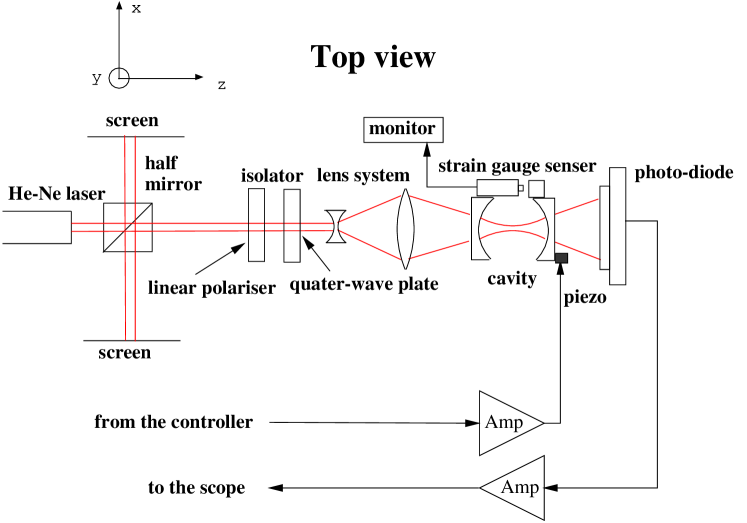
Figure 5: Schematic diagram of the test setup.

3.1 Setup of the experiment

Fig.5 shows a schematic diagram of our test setup. It consists of a He-Ne laser ($\lambda=633$ nm) [9], an isolator, an input lens system, a test cavity, and a photodiode detector. The laser provided a 1 mW beam with a diameter of 0.5 mm ($1/e^{2}$) and a full angular divergence of 1.6 mrad. The transverse spatial mode is ${\rm TEM_{00}}$. In order to avoid a reflected beam to reenter the laser cavity, an optical isolator consisting of a polarizer and a quarter-wave plate was placed at the laser exit. A set of concave and convex lens formed an input lens system, which adjusted the laser beam to match with the Gaussian mode characteristics to the cavity. We used two sets of spherical mirrors [10] of equal curvature ($R=20$mm) with different reflectivity. One set had a nominal reflectivity of $96\%$ and the other set $85\%$. The substrate was BK7 glass ($n=1.519$): its spherical surface was coated with multi-layer dielectric materials and the other flat surface was polished. Thus they acted as a concave lens for input and output light.

These optical elements were installed on adjustable positioners. In particular, the downstream mirror was staged on a piezo translator [11] to scan the mirror along the beam direction $z$. The piezo translator was controlled by a controller [11] and was monitored by a strain gauge sensor with a 10 nm position resolution. We could set the piezo translator manually or scan it by an external voltage signal via the controller. A PIN photodiode [12] was placed at the exit of the cavity. Its output signal was fed into a simple current-to-voltage amplifier whose output was in turn monitored by an oscilloscope. Unless otherwise noted, we tuned the cavity to the fundamental TEM₀₀ mode.

3.2 Measurement of a power enhancement factor

We measured the finesse to evaluate a power enhancement factor. A function generator was used to produce a triangle signal at a frequency of $\sim$100 Hz. It was fed into the piezo controller. Its amplitude was set so that the cavity length $D$ spanned over several free spectral ranges. A typical example of the detector output is shown in Fig.6. We expected the horizontal trace to be proportional to the change in the cavity length $D$ since the piezo translator was driven by a triangle signal. In reality, however, the relation was found to be non-linear due to a hysteresis effect of the piezo translator as well as a mechanical resonance effect of the mirror holder. We measured on the oscilloscope the full width of a single peak $(\delta D(fwhm))$ and the distances to the flanking peaks ($\Delta D$). Then average was taken for the latter to cancel out the non-linear effect.

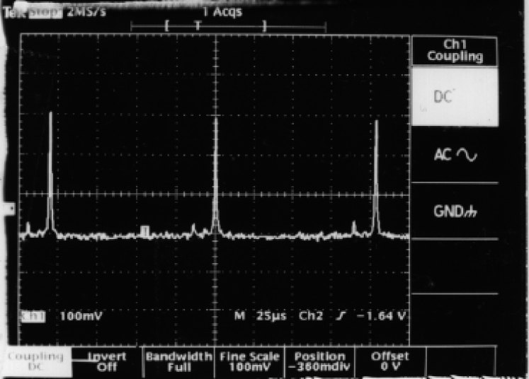
Figure 6: A typical example of the detector output, showing the Airy function.

Assuming that the observed $\Delta D$ was equal to $\lambda/2$, we found the finesse $F$ to be 70 (22) for the mirrors with $R_{m}=96\%(85\%)$. The uncertainty in the measurement, stemming mainly from the non-linear effect in $D$, was estimated to be less than 10%. The measured value should be compared with an expected value of $F$=77 (19). We note that, for our actual application, precise knowledge of an absolute intensity is unnecessary as long as it remains constant since a beam profile would be measured as a relative shape of scattered photon’s counting rate.

3.3 Waist measurement by a shift-rotation method

In order to obtain a beam waist of $\sim\!$$10\mu$m, the cavity length should be set very close to twice of the mirror curvatures ($D\simeq 2R$). The tolerance in $D$ is rather severe; for example, to realize 10% accuracy in the beam waist ($\delta w_{0}/w_{0}=10\%$) for $w_{0}=10\mu$m, the setting error in $D$ must be as small as $\sim\!$$10\mu$m. This would be very difficult, if not impossible, to achieve since construction of the cavity necessarily induces setting errors, especially of glass mirrors. Thus it is highly desirable to measure the cavity length $D$ with sufficient accuracy.

Principle of shift-rotation method

At first, we employed the following method [6] (referred to as a shift-rotation method). Suppose that we have a cavity with unknown cavity length. Suppose also that the cavity is tuned to the fundamental TEM₀₀ mode. Now we shift one of the mirrors laterally. Since the mirrors are both spherical, one can always realign it by rotating the whole cavity. A simple calculation shows that the displacement $x_{\theta}$ and rotation angle $\theta$ are related by

$$\tan(\theta)=\frac{x_{\theta}}{2R-D}.$$

Because the actual mirror is made of concave glass, it acts as a lens. When this effect is taken into account, the formula above should be replaced by

$$\sin(\theta)=n\sin\left\{\arctan\left(\frac{x_{\theta}}{2R-D}\right)\right\}$$ (4)

where $n$ represents the refractive index of the glass substrate. By measuring $x_{\theta}$ and $\theta$, we can determine $2R-D$, and can calculate the beam waist $w_{0}$ with Eq.(2).

Figure 7: Beam waist measurement by shift-rotation method (a) $n{x}_{\theta}/\theta$ vs 2R-D. The solid line is a fit to the data points by a straight line with a unit slope. (b) $\delta{w}_{0}/{w}_{0}$ vs ${w}_{0}$. The beam waist ${w}_{0}$ and its relative error $\delta{w}_{0}/{w}_{0}$ are obtained from measured $n{x}_{\theta}/\theta$ data and its rms deviation.

Results of the measurement

We measured several sets of $x_{\theta}$ and $\theta$ at a fixed cavity length $D$. We then changed cavity length $D$ by moving the stage on which the downstream mirror was mounted. We could trace the amount of a change in $D$ because the stage was driven by a micrometer (attached to the stage in tandem with the piezo translator). Fig.7 (a) shows the results of such measurements. The ordinate is the quantity

$$\frac{x_{\theta}}{\tan\left\{\arcsin\left({\sin\theta}/{n}\right)\right\}}\simeq\frac{nx_{\theta}}{\theta}$$ (5)

where the approximation holds for small $\theta$. The abscissa, labeled as $2R-D$, represents actually $z$ position of the downstream mirror. For a fixed z position, each data point represents the measurement for different sets of $x_{\theta}$ and $\theta$. It can be seen from Eq.(4) that the quantity of Eq.(5) becomes $2R-D$. Thus, ideally all the data points should reside on a straight line with a unit slope. The solid line in the figure represents such a fit. The intersection of the line with the abscissa is then relabeled as origin. Having established the relation between $2R-D$ and the downstream mirror $z$ position, we calculated the beam waist $w_{0}$ with Eq.(2). We also calculated the root-mean-squared (rms) deviation of the data points from the fitted line at fixed $2R-D$. Each rms deviation was then converted to a relative error in $w_{0}$ and is shown in Fig.7 (b). These errors originated from both $x_{\theta}$ and $\theta$ measurements: the former was due mainly to the reading error of the micrometer and the latter to the uncertainty in determining the exact $\theta$ at which the realignment of the optical axis was restored. In this paper, we assign a common error of $\delta w_{0}/w_{0}=0.05$ to the measurements for $w_{0}>20\mu$m. We would like to postpone drawing any conclusion for $w_{0}<20\mu$m .

3.4 Measurement of the far field beam divergence

It can be seen from Eq.(1) that the beam width $w(z)$ in a far field is given by $\displaystyle w(z)\simeq\frac{w_{0}}{z_{0}}z=\frac{\lambda}{\pi w_{0}}z$. Thus a measurement of the output laser profiles gives information on the beam waist $w_{0}$. In particular, the beam intensity, when measured along $x$, reduces to $\displaystyle\frac{1}{\sqrt{e}}$ at $\displaystyle x_{1/\sqrt{e}}=\frac{\lambda z}{2\pi w_{0}}$ from the peak value.

Figure 8: Intensity profile of the output laser beam at the positions of (a) $z={180}$, (b) 230, (c) 280, and (d) 330 mm ($w_{0}=25\mu$m).

Actual measurements were carried out for 4 different values of the beam waist; $w_{0}$=20, 25, 30 and 35 $\mu$m. We call them “nominal” values because these were all determined by the shift-rotation method. We inserted a slit with a horizontal width of $200\mu$m in front of the photodiode. It was then scanned horizontally ($x$ direction) to measure the beam profile. In order to enhance measurement accuracy, we determined the beam widths $\displaystyle x_{1/\sqrt{e}}$ as a function of $z$, and obtained the beam waist $w_{0}$ as a slope of these measurements . Fig.8 shows typical results of such a measurement (for the nominal beam waist of $w_{0}=25\mu$m). Each solid line represents a Gaussian fit to the data points, from which the width $\displaystyle x_{1/\sqrt{e}}$ is determined. Fig.9 shows $\displaystyle x_{1/\sqrt{e}}$ as a function of $z$. Each straight line in the figures is a linear fit to the data points and $w_{0}$ is deduced from its slope.

Figure 9: Measurements of the beam widths $\displaystyle x_{1/\sqrt{e}}$ as a function of $z$ for the nominal beam waist of $w_{0}=$ (a) 35, (b) 30, (c) 25, and (d) 20 $\mu$m. The solid lines are the results of a straight line fit to the data points.

Table 2 shows the summary of the measurements (see the third column). The listed errors are all fitting errors. Note that, since the nominal values are determined by the shift-rotation method, they also have uncertainties, which are listed in the second column. As seen, the two sets of the values agree well with each other. (The fourth column will be explained in the next section.)

3.5 Measurement of higher order transverse modes

The phase of a higher transverse mode ${\rm TEM_{mn}}$ is given by

$$\phi(z)=-\frac{2\pi}{\lambda}z+\left(m+n+1\right)\Phi(z)$$

at $z$ on the beam axis. These transverse modes interfere constructively when the phases at the mirrors ($z=\pm D/2$) satisfy the resonance condition

$$\phi(-D/2)-\phi(D/2)=p\pi$$

where $p$ denotes an integer. A straightforward calculation shows that the condition above is equivalent to

$$D_{p}=\frac{\lambda}{2}\left\{p+\frac{m+n+1}{\pi}\arccos\left(\frac{D_{p}}{R}-1\right)\right\}.$$ (6)

The transmitted beam intensity also exhibits its maximum value when the resonance condition is met. Therefore, the spacing between the adjacent peaks belonging to the same p is given by

$$\Delta D_{p}=D_{p}(m+n=1)-D_{p}(m+n=0)=\frac{\lambda}{2}\left[\frac{1}{\pi}\arccos\left(\frac{D}{R}-1\right)\right]$$ (7)

where the quantity $D_{p}$ in the right hand side of Eq.(6) is replaced by a representative value $D$ since its dependence is weak. Thus we can determine $D$ by measuring the spacing $\Delta D_{p}$ of these peaks. As represented in Eq.(7), we actually measured the spacing between the first excitation mode ($m+n=1$) and the fundamental mode ($m+n=0$).

Table 2: Summary of the beam waist measurements. The nominal values are defined to be those determined by the shift-rotation method. Their uncertainties are listed in the second column.

nominal $w_{0}$	shift-rotation	$a_{1/\sqrt{e}}$ measurement	transverse mode
20.0	$\pm$ 1.0 $\mu$m	20.4 $\pm$ 1.7 $\mu$m	20.1 $\pm$ 0.58 $\mu$m
25.0	$\pm$ 1.3 $\mu$m	24.8 $\pm$ 1.2 $\mu$m	24.9 $\pm$ 0.42 $\mu$m
30.0	$\pm$ 1.5 $\mu$m	31.0 $\pm$ 1.6 $\mu$m	30.0 $\pm$ 0.30 $\mu$m
35.0	$\pm$ 1.8 $\mu$m	37.5 $\pm$ 1.4 $\mu$m	36.4 $\pm$ 0.25 $\mu$m

After confirming the cavity to be in the fundamental TEM₀₀ mode, we detuned the optical axis by shifting one of the mirrors laterally to excite the transverse mode. Fig.10 shows a typical example of an output including higher transverse modes. We determined the spacing between the main peak (the fundamental mode) and its adjacent peak (the first excitation mode) as well as the spacing between two main peaks (a free spectral range). Then we deduced the cavity length $D$ via Eq.(7). The results of the measurements by this method are listed in the fourth column of Table 2. Uncertainty came mainly from reading errors on the oscilloscope and also from non-linearity in $D$.

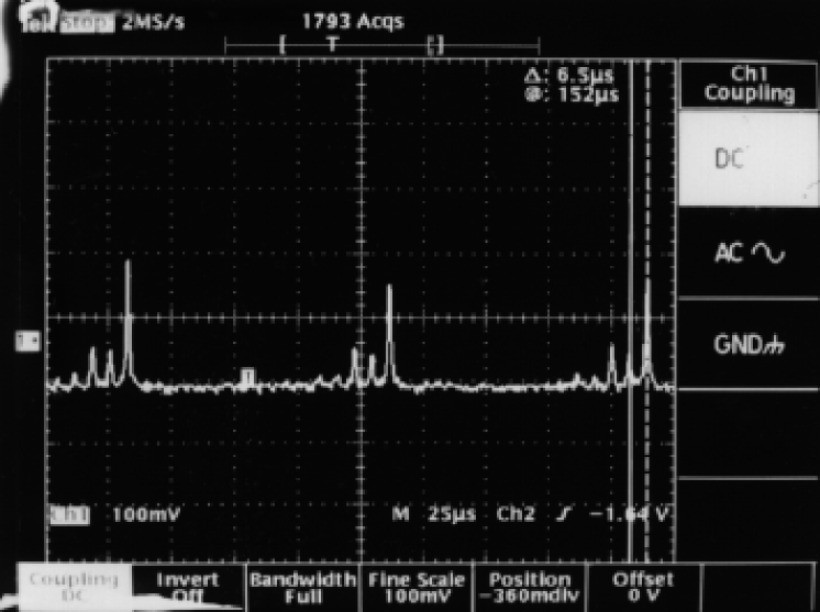
Figure 10: An example of an output including higher transverse modes.

4 Summary and Discussions

We described in this paper a conceptual design of a beam profile monitor for an electron beam with a transverse size of $\sim\!$$60\mu$m (horizontal) and $\sim\!$$10\mu$m (vertical). Specifically, the monitor is intended to diagnose an electron beam in the ATF damping ring at KEK. The monitor works as follows: we realize a very thin ($\sim\!$$10\mu$m) laser wire in an optical cavity. Energetic photons are emitted by the Compton scattering in the direction of the electron beam. The counting rate, measured as a function of the laser beam position, will give information on the electron beam profile.

We calculated the scattered photon energy spectrum (see Fig.2) and the Compton cross section (see Fig.3) for the 1.54 GeV electron beam. Assuming a 10 mW laser and an optical cavity with a beam waist of $10\mu$m and a power enhancement of 100, the expected counting rate is 3.2 kHz (horizontal) and 28.8 kHz (vertical) when scattered photons with energies $>$10 MeV are detected.

A key element of the proposed monitor is the optical cavity, in which a Gaussian beam with a $10\mu$m beam waist must be realized. A power enhancement inside the cavity is an another important parameter to investigate. We thus constructed a test cavity to measure these parameters. The cavity realized the power enhancement of 50 and the beam waist of $20\mu$m. For the beam waist measurement, we employed three independent methods. As seen in Table 2, the results obtained by these methods are consistent with each other. The relative error $\delta w_{0}/w_{0}$ is about 5% by the shift-rotation method, less than 10% by the beam divergence measurement and less than 3% by the higher transverse mode measurement. We measured the finesse $F$ to obtain a power enhancement factor. Using the mirrors with reflectivity of $R_{m}=96\%$, we obtained the enhancement of 50 ($F=70$), which is consistent with the expected value.

Several comments are in order here. First, we have not yet demonstrated a $10\,\mu{\rm m}$ beam waist. The main defect in this test cavity is its mechanical rigidity. In particular the mirror holder (supporting rod) caused disturbing resonant vibration. This can, however, be overcome with a proper cavity design. The second comment is on comparison between the three methods employed to measure the beam waist. The measurement of the beam width $x_{1/\sqrt{e}}$ is very simple and reliable. A newly devised method, the shift-rotation method, gave more accurate results than the beam divergence measurement. However, these methods would not be applicable for an actual cavity installed in an electron beam line. The third one, the observation of higher transverse modes, is simple and the most accurate among the three. Thus this method is best suited to an in-situ measurement. Finally, we comment on a power enhancement factor or an effective power inside the cavity. We demonstrated the enhancement factor of 50. Obviously a higher power is desirable: it would allow us faster measurement and would enable us to study, for example, an electron cooling process and/or a size of an individual bunch. In this regard, we plan to employ a laser with a higher power and mirrors with a higher reflectivity for a prototype monitor. A design work is now underway.

References

- [1] F. Hinode et. al., ATF design and study report, KEK Internal 95-4 (1995)
- [2] Clive Field, SLAC-PUB-6717, Nov. (1994)
- [3] T. Okugi et. al., Phys. Rev. Special Topics- Accelerators and Beam, 2, 022801 (1999)
- [4] Tsumoru Shintake, Nucl. Instr. and Meth., A311 (1992) 453.
- [5] M. C. Ross et. al., Proceeding of XVIII International Linear Accelerator Conference (1998)
- [6] Y. Sakamura, Kyoto University Master Thesis (1997), unpublished.
- [7] G.Giordano et. al., Laser and Particle Beams, 15 (1997) 167.
- [8] A. Yariv, Optical Electronics, Holts, Rinehart and Winston, (New York, 1991), 4th ed.; M. V. Klein and T. E. Furtak, Optics (New York, 1991), 2nd ed.
- [9] Model-117A, Specra Physics INC., Megro-ku, Tokyo 153, Japan
- [10] LCBS-30C10-20-633, Sigma Kohki K.K., Hidaka-shi, Saitama 350-12, Japan
- [11] P-277, PI Company, Tachikawa-shi, Tokyo 190-0012, Japan
- [12] S3071, Hamamatsu Photonics INC., Hamamatsu-shi, Shizuoka 435-91, Japan