SLAC–PUB–8206
July 1999

The lifetimes of $B^{+}$ and $B^{0}$ mesons have been measured using the entire sample of 550,000 hadronic $Z^{0}$ decays collected by the SLD experiment at the SLC between 1993 and 1998. In this paper, we describe the inclusive analysis of the 350,000 hadronic $Z^{0}$ decays collected in 1997-98 with the upgraded SLD vertex detector. In this data period, a high statistics sample of 30903 (20731) charged (neutral) vertices with good charge purity is obtained. The charge purity is enhanced by using the vertex mass, the SLC electron beam polarization (73% for 1997-8) and an opposite hemisphere jet charge technique. Combining the results of this data sample with the results from the earlier data yield the following preliminary values: $\tau_{B^{+}}=1.623\pm 0.020($stat$)\pm 0.034$(syst) ps, $\tau_{B^{0}}=1.589\pm 0.021($stat$)\pm 0.043$(syst) ps, $\tau_{B^{+}}/\tau_{B^{0}}=1.037\pm^{0.025}_{0.024}($stat$)\pm 0.024$(syst).

Paper Contributed to the International Europhysics Conference on High Energy Physics, July 15-21, 1999, Tampere, Finland, Ref. 5-477, and to the XIXth International Symposium on Lepton and Photon Interactions, August 9-14, 1999, Stanford, California, USA.

The spectator model predicts that the lifetime of a heavy hadron depends upon the properties of the constituent weakly decaying heavy quark $Q$ and is independent of the remaining, or spectator, quarks in the hadron. This model fails for the charm hadron system for which the lifetime hierarchy $\tau_{D^{+}}\sim 2.3\tau_{D_{s}^{+}}\sim 2.5\tau_{D^{0}}\sim 5\tau_{\Lambda_{c}^{+}}$ is observed. Since corrections to the spectator model are predicted to scale with $1/m_{Q}^{2}$ the $B$ meson lifetimes are expected to differ by less than 10% [1]. Hence a measurement of the $B^{+}$ and $B^{0}$ lifetimes provides a test of this prediction. In addition, specific $B$ meson lifetimes are needed for many important measurements, e.g. to determine the element $V_{cb}$ of the CKM matrix.

An analysis has been reported using the 1993-5 data sample of 150,000 hadronic $Z^{0}$ decays collected with the original CCD vertex detector (VXD2) as well as with the first 50,000 hadronic $Z^{0}$ decays collected in 1996 using the upgraded vertex detector (VXD3) [2]. In this paper we describe the analysis of the additional 350,000 hadronic $Z^{0}$ decays collected in the 1997-1998 run by the SLD detector at the SLC, and combine these results with those from the previous work[3]. The excellent 3-D vertexing capabilities of SLD are exploited with an inclusive topological vertexing technique [4] to identify $B$ hadron vertices produced in hadronic $Z^{0}$ decays with high efficiency (This inclusive technique has the advantage of very efficient $B$ vertex reconstruction since most $B$ decays are used). The decay length is measured using the reconstructed vertex location while the $B$ hadron charge is determined from the total charge of the tracks associated with the vertex. Knowledge of the average energy of $B$-hadrons produced in $Z^{0}$ decays, in conjuction with the decay length, lets one infer the $B$ lifetime.

The components of the SLD utilized by this analysis are the Central Drift Chamber (CDC)[5] for charged track reconstruction and momentum measurement and the CCD pixel Vertex Detector (VXD)[2, 5] for precise position measurements near the interaction point. These systems are immersed in the 0.6 T field of the SLD solenoid. Charged tracks reconstructed in the CDC are linked with pixel clusters in the VXD by extrapolating each track and selecting the best set of associated clusters[5]. For VXD3 the track impact parameter resolutions at high momentum are 9 $\mu$m and 11 $\mu$m in the $r\phi$ and $rz$ projections respectively ($z$ points along the beam direction), while multiple scattering contributions are $33\,\mu$m $/(p\,{\rm sin}^{3/2}\theta)$ in both projections (where the momentum $p$ is expressed in GeV/c).

The centroid of the micron-sized SLC Interaction Point (IP) in the $r\phi$ plane is reconstructed with a measured precision of $\sigma_{IP}=(4\pm 2)\,\mu$m using tracks in sets of $\sim 30$ sequential hadronic $Z^{0}$ decays. The median $z$ position of tracks at their point of closest approach to the IP in the $r\phi$ plane is used to determine the $z$ position of the $Z^{0}$ primary vertex on an event-by-event basis. A precision of $\sim 30\,\mu$m on this quantity is estimated using $Z^{0}\rightarrow b\overline{b}$ Monte Carlo simulation for VXD3.

The simulated $Z^{0}\rightarrow q\>{\overline{q}}$ events are generated using JETSET 7.4 [6]. The $B$ meson decays are simulated using the CLEO $B$ decay model [7] tuned to reproduce the spectra and multiplicities of charmed hadrons, pions, kaons, protons and leptons as measured at the $\Upsilon$(4S) by ARGUS and CLEO [8]. The branching fractions of the charm hadrons are tuned to the existing measurements [9]. The $B$ mesons and baryons are generated with lifetimes of $\tau_{B^{+}}=1.64$ ps, $\tau_{B^{0}}=1.55$ ps, $\tau_{B^{0}_{s}}=1.57$ ps, and $\tau_{\Lambda_{b}}=1.22$ ps. The $b$-quark fragmentation follows the Peterson et al. parameterization [10]; the mean value of the fragmentation function in the MC generation was $0.698$. The SLD detector is simulated using GEANT 3.21 [11].

Hadronic $Z^{0}$ event selection requires at least 7 CDC tracks which pass within 5 cm of the IP in $z$ at the point of closest approach to the beam and which have momentum transverse to the beam direction $p_{T}>$200 MeV/$c$. The sum of the energy of the charged tracks passing these cuts must be greater than 18 GeV. These requirements remove background from $Z^{0}\to l^{+}l^{-}$ events and two-photon interactions. In addition, the thrust axis determined from energy clusters in the calorimeter must have $\left|\cos\theta\right|<0.85$. within the acceptance of the vertex detector. These requirements yield a sample of $\sim 267,500$ hadronic $Z^{0}$ decays for the 1997-98 datset.

Good quality tracks used for vertex finding must have a CDC hit at a radius$<$39 cm, and have $\geq$23 hits to insure that the lever arm provided by the CDC is appreciable. The CDC tracks must have $p_{T}>$250 MeV/$c\>$ and extrapolate to within 1 cm of the IP in $r\phi$ and within 1.5 cm in $z$ to eliminate tracks which arise from interaction with the detector material. The fit of the track must satisfy $\chi^{2}/$d.o.f.$<8$. At least two good VXD3 links are required, and the combined CDC/VXD fit must also satisfy $\chi^{2}/$d.o.f.$<8$.

The topological vertex reconstruction is applied separately to the tracks in each hemisphere (defined with respect to the event thrust axis). The vertexing algorithm is described in detail in Ref. [4] and summarized here. The vertices are reconstructed in 3-D coordinate space by defining a vertex function $V({\bf r})$ at each position ${\bf r}$. The helix parameters for each track $i$ are used to describe the 3-D track trajectory as a Gaussian tube $f_{i}({\bf r})$, where the width of the tube is the uncertainty in the measured track location close to the IP. A function $f_{0}({\bf r})$ is used to describe the location and uncertainty of the IP. $V({\bf r})$ is defined as a function of $f_{0}({\bf r})$ and the $f_{i}({\bf r})$ such that it is small in regions where fewer than two tracks (required for a vertex) have significant $f_{i}({\bf r})$, and large in regions of high track multiplicity. Maxima are found in $V({\bf r})$ and clustered into resolved spatial regions. Tracks are associated with these regions to form a set of topological vertices.

The efficiency for reconstructing at least one secondary vertex in a $b$ hemisphere is $\sim 67$% for VXD3. The efficiency falls at shorter decay length as it becomes harder to resolve the secondary vertex from the IP. For hemispheres containing secondary vertices, the ‘seed’ vertex is chosen to be the one with the highest $V({\bf r})$ value. Vertices consistent with a $K^{0}_{s}\to\pi^{+}\pi^{-}$ decay, within a 14 MeV invariant mass window, are excluded from the seed vertex selection and the two tracks are discarded.

A vertex axis is formed by a straight line joining the IP to the seed vertex. The 3-D distance of closest approach of a track to the vertex axis, T, and the distance from the IP along the vertex axis to this point, L, are calculated for all quality tracks. Monte Carlo studies show that tracks which are not directly associated with the seed vertex but which pass T$<0.1$ cm and L$/$D$>0.3$ (where D is the distance from the IP to the seed vertex) are more likely to have been produced by the $B$ decay sequence than to have an alternative origin. Hence such tracks are added to the set of tracks in the seed vertex to form the candidate $B$ decay vertex, containing tracks from both the $B$ and cascade $D$ decays. This set of tracks is fitted to a common vertex. If the probability of the vertex fit is greater than 5% the $B$ decay location is taken to be the fitted vertex location. Since the vertex includes tracks form both the $B$ and cascade charm decay points the fit probability distribution is not flat and $\sim 65$% of vertices reconstructed have a fit probability below 5%. The reconstruction of the $B$ decay location in this case is improved by dividing the tracks (if there are at least three) into two ‘sub-vertices’ by selecting the combination of tracks with maximum two sub-vertex fit probability. The $B$ decay location is given by the sub-vertex closest to the IP, reducing systematic dependence upon the physics of the $B\to D$ decay. The distance from the IP to the $B$ decay location is the reconstructed decay length. Since the purity of the $B$ charge reconstruction is lower for decays close to the IP, where tracks are more likely to be wrongly assigned, decay lengths are required to be $>1$ mm. To avoid using the vertices of tracks originating from interactions with the detector material, the distance of the decay vertex from the beamline is required to be $<22$ mm, i.e. more than $1$ mm inside the SLC beampipe.

Figure 1: (a) $M_{P_{T}}$ of reconstructed vertex for 1997-98 data (points) and Monte Carlo (histogram), (b) $B^{+}$ fraction in the charged sample, (c) $B^{0}$ fraction in the neutral sample.

The mass $M$ of the reconstructed vertex is calculated by assuming each track has the mass of a pion. The transverse component $P_{T}$ of the total momentum of vertex tracks relative to the vertex axis is calculated in order to determine the $P_{T}$ corrected mass:

$$M_{P_{T}}=\sqrt{M^{2}+P^{2}_{T}}+|P_{T}|.$$ (1)

This quantity is the minimum mass the decaying hadron could have in order to produce a vertex with the quantities $M$ and $P_{T}$. The direction of the vertex axis is varied within the $1\sigma$ limits constraining the axis at the measured IP and reconstructed seed vertex such that the $P_{T}$ is minimized within this variation. This procedure prevents non-$B$ background vertices acquiring a high $M_{P_{T}}$ due to a fluctuation in the measured $P_{T}$. The accurate 3-D vertexing and precisely measured IP at SLD allow significant gain in the $b$-tag efficiency with high purity using this technique [12].

A comparison of the distribution of $M_{P_{T}}$ in data and Monte Carlo is shown in Fig. 1(a). Vertices from $K^{0}_{s}$ decays surviving the $K^{0}_{s}$ rejection can be seen around $0.5$ GeV/$c^{2}$. This figure shows that a large fraction of the charm and light flavor contamination in the sample is eliminated by requiring $M_{P_{T}}>2$ GeV/$c^{2}$. It is also required that $M_{P_{T}}<5.2$ GeV/$c^{2}$ since vertices with $M_{P_{T}}$ greater than the $B$ meson mass are likely to contain background tracks. These cuts yield a sample with $b$ hemisphere purity of $\sim$ 98% with an efficiency of 38%. The average $B$ decay vertex multiplicity is 5.0 tracks.

To improve the $B$ hadron charge reconstruction, tracks which fail the initial selection but have $p_{T}>$ 200 MeV/$c$ and $\sqrt{\sigma_{r\phi}^{2}+\sigma_{rz}^{2}}<700\,\mu$m, where $\sigma_{r\phi}$ ($\sigma_{rz}$) is the uncertainty in the track position in the $r\phi$ ($rz$) plane close to the IP, are considered as decay track candidates. The charge of these tracks which pass the cuts T$<\,0.1$ cm and L$/$D$>0.3$ is added to the $B$ decay charge. On average, 0.4 tracks pass these criteria in $b$ hemispheres. These lower quality tracks are used only to improve the charge reconstruction.

Figure 2: Reconstructed vertex charge for data (points) and Monte Carlo (histogram) for the 1997-98 dataset.

Fig. 2 shows a comparison of the reconstructed charge between data and Monte Carlo for the 1997-1998 dataset. At this stage the charged sample consists of 30903 vertices with vertex charge equal to $\pm$ 1,2 or 3, while the neutral sample consists of 20731 vertices with charge equal to 0. Monte Carlo studies indicate that the charged sample is 97.0% pure in $B$ hadrons consisting of 57.2% $B^{+}$, 32.0% $B^{0}$, 8.1% $B_{s}^{0}$, and 4.5% $B$ baryons. (Charge conjugation is implied throughout this paper with the exception of the notation $B_{+}$ and $B_{-}$ introduced later to distinguish the charged mesons $B(\overline{b}u)$ and $B(b\overline{u})$ and respectively.) Similarly, the neutral sample is 98.3% pure in $B$ hadrons consisting of 21.9% $B^{+}$, 55.0% $B^{0}$, 15.6% $B_{s}^{0}$ and 7.6% $B$ baryons. The statistical precision of the measurement depends on the separation between the $B^{+}$ and $B^{0}$ in these samples.

The lifetime measurement relies on the ability to separate $B^{+}$ and $B^{0}$ decays by making use of the vertex charge. Monte Carlo studies show that the purity of the charge reconstruction is more likely to be eroded by losing tracks from the $B$ decay chain through track selection inefficiencies and track mis-assignment than by gaining mis-assigned tracks originating from the primary or other background to the $B$ decay. Furthermore, the decays which are missing some $B$ tracks tend to have lower vertex mass as well as lower charge purity. Fig. 1(b) and (c) show the fraction of $B^{+}$ decays in the charged sample and the fraction of $B^{0}$ decays in the neutral sample respectively for MC. The probability for the vertex to originate from a positively charged, neutral or negatively charged $B$ meson is denoted as $P_{c}(B_{+})$, $P_{c}(B^{0})$ and $P_{c}(B_{-})$ respectively, normalized such that $P_{c}(B_{+})+P_{c}(B^{0})+P_{c}(B_{-})=1$. Vertices are given a weight, $w$, according to their analyzing power for separating $B^{+}$ and $B^{0}$ decays: $w=\left|2P_{c}(B^{+})-1\right|$, where $P_{c}(B^{+})=P_{c}(B_{+})+P_{c}(B_{-})$. The probabilities, and hence the weight, are a function of $M_{P_{T}}$.

The charge reconstruction in Fig. 2 shows good agreement between data and MC. A further check is made using the SLC electron beam polarization. The polarized forward-backward asymmetry ${A}_{FB}(P_{e},\cos\theta)$ can be described by

$${A}_{FB}(P_{e},\cos\theta)=2A_{b}~{}{{A_{e}-P_{e}}\over{1-A_{e}P_{e}}}~{}{{\cos\theta}\over{1+\cos^{2}\theta}}~{},$$ (2)

where $A_{b}=0.94$ and $A_{e}=0.155$ (Standard Model values), $P_{e}$ is the electron beam longitudinal polarization, and $\theta$ is the angle between the thrust axis and the electron beam direction (the thrust axis is signed such that it points in the same hemisphere as the reconstructed vertex). Using negative (positive) vertex charge, with vertices weighted by the $M_{P_{T}}$ dependent analyzing power, to tag the $b$ ($\overline{b}$) quark flavor the resulting forward backward asymmetry is sensitive to the accuracy of the vertex charge reconstruction. Good agreement between data and MC can be seen in Fig. 3 for the 1997-8 data, indicating that the MC adequately reproduces the charge reconstruction purity of the data. (Random vertex charge assignment would generate distributions with no signed $\cos\theta$ asymmetry.)

Figure 3: Distribution of cos$\theta$ signed by ($P_{e}\times$ vertex charge) for 1997-8 data (points) and Monte Carlo (histogram).

The polarized forward-backward asymmetry can be used to tag the initial state $b$ or $\overline{b}$ flavor of the hemisphere. The initial state $b/\overline{b}$ tag is also used to enhance the charged sample purity by giving a higher (lower) weight to the $B^{+}$ hypothesis if the vertex charge agrees (disagrees) with the $b/\overline{b}$ tag. The probability for correctly tagging a $b$ quark at production using the $e^{-}$ beam polarization is expressed as

$$P_{A}(b)={{1+A_{FB}(P_{e},\cos\theta)}\over{2}}~{}.$$ (3)

A jet charge technique is used in addition to the polarized forward-backward asymmetry. For this tag, tracks in the hemisphere opposite that of the reconstructed vertex are selected. These tracks are required to have momentum transverse to the beam axis $p_{\perp}>150$ MeV/c, total momentum $p<50$ GeV/c, impact parameter in the plane perpendicular to the beam axis $\delta<2$ cm, distance between the primary vertex and the track at the point of closest approach along the beam axis $\Delta z<10$ cm, and $|\cos\theta|<0.87$. With these tracks, an opposite hemisphere momentum-weighted track charge is defined as

$$Q_{opp}=\sum_{i}q_{i}\left|\vec{p}_{i}\cdot\hat{T}\right|^{\kappa}~{},$$ (4)

where $q_{i}$ is the electric charge of track $i$, $\vec{p}_{i}$ its momentum vector, $\hat{T}$ is the thrust axis direction, and $\kappa$ is a coefficient chosen to be 0.5 to maximize the separation between $b$ and $\overline{b}$ quarks. The probability for correctly tagging a $b$ quark in the initial state of the vertex hemisphere can be parameterized as

$$P_{Q}(b)={{1}\over{1+e^{\alpha Q_{opp}}}}~{},$$ (5)

where the coefficient $\alpha=-0.27$ as determined using the Monte Carlo simulation. This technique is independent of the polarized forward-backward asymmetry tag. The average purity of the $b/\overline{b}$ tag is $\sim 72$% using the forward backward asymmetry ($\left|P_{e}\right|=73$%) and 67% for the jet charge technique.

The two initial state tags can be combined to form an overall initial state tag with $b/\overline{b}$ quark probability $P_{i}(b)/P_{i}(\overline{b})$ (a function of $P_{e}$, $\cos\theta$ and $Q_{opp}$). This probability is then combined with that obtained from the vertex charge reconstruction (a function of $M_{P_{T}}$) to determine the overall probability of a $B^{+}$ or $B^{0}$ decay:

$$P(B^{+})={{P_{c}(B_{+})P_{i}(\overline{b})+P_{c}(B_{-})P_{i}(b)}\over{P_{c}(B_{+})P_{i}(\overline{b})+P_{c}(B_{-})P_{i}(b)+0.5\times P_{c}(B^{0})}}$$ (6)

where $B_{+}$ and $B_{-}$ denote the positively and negatively charged $B$ mesons separately and $P(B^{0})=1-P(B^{+})$. If the probability $P(B^{+})>P(B^{0})$ the vertex is classified as charged, otherwise it is added to the neutral sample. In either case it is weighted by the analyzing power $w=\left|2P(B^{+})-1\right|$. Including the initial state tag information enhances the statistical power of the analysis by $\sim$20%.

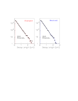
Figure 4: Decay length distributions for the 1997-8 data (points) and best fit Monte Carlo (histogram).

The $B^{+}$ and $B^{0}$ lifetimes are extracted from the decay length distributions of the $B$ vertices in the charged and neutral samples using a binned $\chi^{2}$ fit. These distributions are fitted simultaneously to determine the $B^{+}$ and $B^{0}$ lifetimes. For each set of parameter values, Monte Carlo decay length distributions are obtained by reweighting entries from generated $B^{+}$ and $B^{0}$ decays in the original Monte Carlo decay length distributions with $W(t,\tau)=\left(\frac{1}{\tau}~{}e^{-t/\tau}\right)/\left(\frac{1}{\tau_{gen}}~{}e^{-t/\tau_{gen}}\right)$, where $\tau$ is the desired $B^{+}$ or $B^{0}$ lifetime, $\tau_{gen}$ is the average lifetime generated in the Monte Carlo, and $t$ is the proper time of each decay. The fit then compares the decay length distributions from the data with the reweighted Monte Carlo distributions. Fig. 4 shows the reconstructed decay length for data and best fit MC for the 1997-8 data and the charged and neutral samples. (The fits are made using histograms in which the bin size increases with decay length such that the number of entries per bin remains approximately constant.) The fit to the 1997-8 data sample yields lifetimes of $\tau_{B^{+}}=1.657\pm 0.023$ ps and $\tau_{B^{0}}=1.578\pm 0.024$ ps, with a ratio of $\tau_{B^{+}}/\tau_{B^{0}}$ $=1.049^{+0.028}_{-0.027}$ and a $\chi^{2}/$d.o.f. = 79.8/76. These results are then corrected to correspond to b-fragmentation with a mean scaled energy $<X_{E}>=0.714$ [13], a $B_{s}^{0}$ lifetime of 1.49 ps, and a b-baryon fraction of 10.2% [9]. The corrected results for 1997-98 are: $\tau_{B^{+}}=1.613\pm 0.023$ ps and $\tau_{B^{0}}=1.565\pm 0.024$ ps, with a ratio of $\tau_{B^{+}}/\tau_{B^{0}}$ $=1.030^{+0.028}_{-0.027}$.

To account for a discrepancy between data and Monte Carlo in the fraction of tracks passing the selection criteria, a $\sim$4% tracking efficiency correction with dependence on track momenta and angles is applied to the simulation [5]. The corrected Monte Carlo is used in the lifetime fits, with the effect of the entire correction taken as the systematic error.

The physics modeling systematic uncertainties were determined as follows. The mean fragmentation energy $<\!\!x_{E}\!\!>$ of the $B$ hadron [13] and the shape of the $x_{E}$ distribution [14] were varied. Since the fragmentation is assumed to be identical for the $B^{+}$ and $B^{0}$ mesons, this uncertainty has little effect on the lifetime ratio. The four branching fractions for $B^{+}/B^{0}\rightarrow\overline{D^{0}}/D^{-}X$ were varied by twice the uncertainty given in Ref. [15] for $B\rightarrow\overline{D^{0}}/D^{-}X$. The fraction of $B^{+}/B^{0}$ decays producing a $D\overline{D}$ pair was also varied. The average $B^{+}$ and $B^{0}$ decay multiplicity was varied by $\pm 0.3$ tracks [16] in an anticorrelated manner. Uncertainties in the $B_{s}^{0}$ and $B$ baryon lifetimes and production fractions mostly affect the $B^{0}$ lifetime since the neutral $B_{s}^{0}$ and $B$ baryon are a more significant background for the $B^{0}$ decays. The systematic errors due to uncertainties in charmed meson decay topology were estimated by changing the Monte Carlo $D$ decay charged multiplicity and $K^{0}$ production according to the uncertainties in experimental measurements [17]. The effect of varying the lifetime of charm hadrons ($D^{+}$, $D^{0}$, $D_{s}$, $\Lambda_{c}$), as well as their momentum spectra in the $B$ decay rest frame was found to be negligible.

The fitting uncertainties were determined by varying the bin size used in the decay length distributions, and by modifying the cuts on the minimum decay length (no cut–2 mm) and maximum radius cuts (20 mm–no cut) used in the fit. Fit results are consistent within statistics for these variations, but a systematic error is conservatively assigned using the RMS variation of the results.

Table 1 summarizes the systematic errors on the $B^{+}$ and $B^{0}$ lifetimes and their ratio for the 1997-1998 dataset.

Table 1: Summary of systematic uncertainties in the $B^{+}$ and $B^{0}$ lifetimes and their ratio for the 1997-98 dataset.

Systematic Error		$\Delta\tau_{B^{+}}$	$\Delta\tau_{B^{0}}$	$\Delta\frac{\tau_{B^{+}}}{\tau_{B^{0}}}$
		(ps)	(ps)
	Detector Modeling
Tracking efficiency		0.005	0.011	0.008
Tracking resolution		0.003	0.003	0.003
	Physics Modeling
$b$ fragmentation	0.714 $\pm$ 0.008	0.025	0.030	$<$0.003
	$x_{E}$ shape	0.011	0.009	$<$0.003
BR($B\to DX$)		0.005	0.009	0.007
BR($B\to D\overline{D}X$)	0.19 $\pm$ 0.05	0.015	0.014	0.016
$B$ decay multiplicity	5.3 $\pm$ 0.3	$<$0.003	$<$0.003	$<$0.003
$B_{s}^{0}$ fraction	0.115 $\pm$ 0.020	0.003	$<$0.003	$<$0.003
$B$ baryon fraction	0.102 $\pm$ 0.020	0.004	0.017	0.008
$B_{s}^{0}$ lifetime	1.49 $\pm$ 0.06 ps	$<$0.003	0.014	0.009
$B$ baryon lifetime	1.22 $\pm$ 0.05 ps	$<$0.003	0.005	0.003
$D$ decay multiplicity		0.003	0.005	0.006
$D$ decay $K^{0}$ yield		$<$0.003	0.008	0.004
	Monte Carlo and Fitting
Fitting systematics		0.010	0.009	0.006
MC statistics		0.006	0.006	0.007
TOTAL		0.033	0.044	0.026

Finally, the 1993-95 and 1996 results [3] are then combined with these more recent results, taking into account correlated uncertainties. For the earlier data sets, the results have been adjusted so that their assumed values for the b-baryon fraction and the mean of the fragmentation function agrees with this current analysis. The combination of the 1993-5, 1996, and 1997-98 data samples yield lifetimes of $\tau_{B^{+}}=1.623\pm 0.020$ ps and $\tau_{B^{0}}=1.585\pm 0.031$ ps, with a ratio of $\tau_{B^{+}}/\tau_{B^{0}}$ $=1.037^{+0.025}_{-0.024}$. The combined systematics for the 1993-98 data are shown in Table 2.

Table 2: Summary of systematic uncertainties in the $B^{+}$ and $B^{0}$ lifetimes and their ratio for the combined 1993-8 data.

Systematic Error		$\Delta\tau_{B^{+}}$	$\Delta\tau_{B^{0}}$	$\Delta\frac{\tau_{B^{+}}}{\tau_{B^{0}}}$
		(ps)	(ps)
	Detector Modeling
Tracking efficiency		0.004	0.004	0.005
Tracking resolution		0.003	0.003	0.003
	Physics Modeling
$b$ fragmentation	0.714 $\pm$ 0.008	0.025	0.028	.004
	$x_{E}$ shape	0.011	0.010	$<$0.003
BR($B\to DX$)		0.005	0.009	0.007
BR($B\to D\overline{D}X$)	0.19 $\pm$ 0.05	0.013	0.012	0.014
$B$ decay multiplicity	5.3 $\pm$ 0.3	$<$0.003	$<$0.003	$<$0.003
$B_{s}^{0}$ fraction	0.115 $\pm$ 0.020	0.005	$<$0.003	$<$0.003
$B$ baryon fraction	0.102 $\pm$ 0.020	0.005	0.017	0.008
$B_{s}^{0}$ lifetime	1.49 $\pm$ 0.06 ps	$<$0.003	0.014	0.009
$B$ baryon lifetime	1.22 $\pm$ 0.05 ps	$<$0.003	0.005	0.003
$D$ decay multiplicity		0.005	0.006	0.008
$D$ decay $K^{0}$ yield		0.003	0.009	0.006
	Monte Carlo and Fitting
Fitting systematics		0.008	0.007	0.005
MC statistics		0.005	0.005	0.006
TOTAL		0.034	0.043	0.024

In summary, from the entire 550,000 $Z^{0}$ decays collected by SLD between 1993 and 1998, the $B^{+}$ and $B^{0}$ lifetimes have been measured using an inclusive topological technique. The analysis of the 1997-98 dataset of 350,000 decays, discussed above, isolates 51634 $B$ hadron candidates with good charge purity enhanced by the vertex mass, $e^{-}$ beam polarization and opposite hemisphere jet charge information. These results have been combined with the earlier 1993-96 measurements to yield the following preliminary results:

$$\tau_{B^{+}} = 1.623\pm 0.020(\mbox{stat})\pm 0.034(\mbox{syst})\mbox{~{}ps},$$

$$\tau_{B^{0}} = 1.585\pm 0.021(\mbox{stat})\pm 0.043(\mbox{syst})\mbox{~{}ps},$$

$$\frac{\tau_{B^{+}}}{\tau_{B^{0}}} = 1.037\pm^{0.025}_{0.024}(\mbox{stat})\pm 0.024(\mbox{syst}).$$

These results are consistent with the expectation that the $B^{+}$ lifetime is up to 10% greater than that of the $B^{0}$ and have the best statistical accuracy among current measurements [18].

We thank the personnel of the SLAC accelerator department and the technical staffs of our collaborating institutions for their outstanding efforts.

^∗∗ List of Authors

Kenji Abe,⁽²¹⁾ Koya Abe,⁽³³⁾ T. Abe,⁽²⁹⁾ I. Adam,⁽²⁹⁾ T. Akagi,⁽²⁹⁾ H. Akimoto,⁽²⁹⁾ N.J. Allen,⁽⁵⁾ W.W. Ash,⁽²⁹⁾ D. Aston,⁽²⁹⁾ K.G. Baird,⁽¹⁷⁾ C. Baltay,⁽⁴⁰⁾ H.R. Band,⁽³⁹⁾ M.B. Barakat,⁽¹⁶⁾ O. Bardon,⁽¹⁹⁾ T.L. Barklow,⁽²⁹⁾ G.L. Bashindzhagyan,⁽²⁰⁾ J.M. Bauer,⁽¹⁸⁾ G. Bellodi,⁽²³⁾ A.C. Benvenuti,⁽³⁾ G.M. Bilei,⁽²⁵⁾ D. Bisello,⁽²⁴⁾ G. Blaylock,⁽¹⁷⁾ J.R. Bogart,⁽²⁹⁾ G.R. Bower,⁽²⁹⁾ J.E. Brau,⁽²²⁾ M. Breidenbach,⁽²⁹⁾ W.M. Bugg,⁽³²⁾ D. Burke,⁽²⁹⁾ T.H. Burnett,⁽³⁸⁾ P.N. Burrows,⁽²³⁾ R.M. Byrne,⁽¹⁹⁾ A. Calcaterra,⁽¹²⁾ D. Calloway,⁽²⁹⁾ B. Camanzi,⁽¹¹⁾ M. Carpinelli,⁽²⁶⁾ R. Cassell,⁽²⁹⁾ R. Castaldi,⁽²⁶⁾ A. Castro,⁽²⁴⁾ M. Cavalli-Sforza,⁽³⁵⁾ A. Chou,⁽²⁹⁾ E. Church,⁽³⁸⁾ H.O. Cohn,⁽³²⁾ J.A. Coller,⁽⁶⁾ M.R. Convery,⁽²⁹⁾ V. Cook,⁽³⁸⁾ R.F. Cowan,⁽¹⁹⁾ D.G. Coyne,⁽³⁵⁾ G. Crawford,⁽²⁹⁾ C.J.S. Damerell,⁽²⁷⁾ M.N. Danielson,⁽⁸⁾ M. Daoudi,⁽²⁹⁾ N. de Groot,⁽⁴⁾ R. Dell’Orso,⁽²⁵⁾ P.J. Dervan,⁽⁵⁾ R. de Sangro,⁽¹²⁾ M. Dima,⁽¹⁰⁾ D.N. Dong,⁽¹⁹⁾ M. Doser,⁽²⁹⁾ R. Dubois,⁽²⁹⁾ B.I. Eisenstein,⁽¹³⁾ I.Erofeeva,⁽²⁰⁾ V. Eschenburg,⁽¹⁸⁾ E. Etzion,⁽³⁹⁾ S. Fahey,⁽⁸⁾ D. Falciai,⁽¹²⁾ C. Fan,⁽⁸⁾ J.P. Fernandez,⁽³⁵⁾ M.J. Fero,⁽¹⁹⁾ K. Flood,⁽¹⁷⁾ R. Frey,⁽²²⁾ J. Gifford,⁽³⁶⁾ T. Gillman,⁽²⁷⁾ G. Gladding,⁽¹³⁾ S. Gonzalez,⁽¹⁹⁾ E.R. Goodman,⁽⁸⁾ E.L. Hart,⁽³²⁾ J.L. Harton,⁽¹⁰⁾ K. Hasuko,⁽³³⁾ S.J. Hedges,⁽⁶⁾ S.S. Hertzbach,⁽¹⁷⁾ M.D. Hildreth,⁽²⁹⁾ J. Huber,⁽²²⁾ M.E. Huffer,⁽²⁹⁾ E.W. Hughes,⁽²⁹⁾ X. Huynh,⁽²⁹⁾ H. Hwang,⁽²²⁾ M. Iwasaki,⁽²²⁾ D.J. Jackson,⁽²⁷⁾ P. Jacques,⁽²⁸⁾ J.A. Jaros,⁽²⁹⁾ Z.Y. Jiang,⁽²⁹⁾ A.S. Johnson,⁽²⁹⁾ J.R. Johnson,⁽³⁹⁾ R.A. Johnson,⁽⁷⁾ T. Junk,⁽²⁹⁾ R. Kajikawa,⁽²¹⁾ M. Kalelkar,⁽²⁸⁾ Y. Kamyshkov,⁽³²⁾ H.J. Kang,⁽²⁸⁾ I. Karliner,⁽¹³⁾ H. Kawahara,⁽²⁹⁾ Y.D. Kim,⁽³⁰⁾ M.E. King,⁽²⁹⁾ R. King,⁽²⁹⁾ R.R. Kofler,⁽¹⁷⁾ N.M. Krishna,⁽⁸⁾ R.S. Kroeger,⁽¹⁸⁾ M. Langston,⁽²²⁾ A. Lath,⁽¹⁹⁾ D.W.G. Leith,⁽²⁹⁾ V. Lia,⁽¹⁹⁾ C.Lin,⁽¹⁷⁾ M.X. Liu,⁽⁴⁰⁾ X. Liu,⁽³⁵⁾ M. Loreti,⁽²⁴⁾ A. Lu,⁽³⁴⁾ H.L. Lynch,⁽²⁹⁾ J. Ma,⁽³⁸⁾ M. Mahjouri,⁽¹⁹⁾ G. Mancinelli,⁽²⁸⁾ S. Manly,⁽⁴⁰⁾ G. Mantovani,⁽²⁵⁾ T.W. Markiewicz,⁽²⁹⁾ T. Maruyama,⁽²⁹⁾ H. Masuda,⁽²⁹⁾ E. Mazzucato,⁽¹¹⁾ A.K. McKemey,⁽⁵⁾ B.T. Meadows,⁽⁷⁾ G. Menegatti,⁽¹¹⁾ R. Messner,⁽²⁹⁾ P.M. Mockett,⁽³⁸⁾ K.C. Moffeit,⁽²⁹⁾ T.B. Moore,⁽⁴⁰⁾ M.Morii,⁽²⁹⁾ D. Muller,⁽²⁹⁾ V. Murzin,⁽²⁰⁾ T. Nagamine,⁽³³⁾ S. Narita,⁽³³⁾ U. Nauenberg,⁽⁸⁾ H. Neal,⁽²⁹⁾ M. Nussbaum,⁽⁷⁾ N. Oishi,⁽²¹⁾ D. Onoprienko,⁽³²⁾ L.S. Osborne,⁽¹⁹⁾ R.S. Panvini,⁽³⁷⁾ C.H. Park,⁽³¹⁾ T.J. Pavel,⁽²⁹⁾ I. Peruzzi,⁽¹²⁾ M. Piccolo,⁽¹²⁾ L. Piemontese,⁽¹¹⁾ K.T. Pitts,⁽²²⁾ R.J. Plano,⁽²⁸⁾ R. Prepost,⁽³⁹⁾ C.Y. Prescott,⁽²⁹⁾ G.D. Punkar,⁽²⁹⁾ J. Quigley,⁽¹⁹⁾ B.N. Ratcliff,⁽²⁹⁾ T.W. Reeves,⁽³⁷⁾ J. Reidy,⁽¹⁸⁾ P.L. Reinertsen,⁽³⁵⁾ P.E. Rensing,⁽²⁹⁾ L.S. Rochester,⁽²⁹⁾ P.C. Rowson,⁽⁹⁾ J.J. Russell,⁽²⁹⁾ O.H. Saxton,⁽²⁹⁾ T. Schalk,⁽³⁵⁾ R.H. Schindler,⁽²⁹⁾ B.A. Schumm,⁽³⁵⁾ J. Schwiening,⁽²⁹⁾ S. Sen,⁽⁴⁰⁾ V.V. Serbo,⁽²⁹⁾ M.H. Shaevitz,⁽⁹⁾ J.T. Shank,⁽⁶⁾ G. Shapiro,⁽¹⁵⁾ D.J. Sherden,⁽²⁹⁾ K.D. Shmakov,⁽³²⁾ C. Simopoulos,⁽²⁹⁾ N.B. Sinev,⁽²²⁾ S.R. Smith,⁽²⁹⁾ M.B. Smy,⁽¹⁰⁾ J.A. Snyder,⁽⁴⁰⁾ H. Staengle,⁽¹⁰⁾ A. Stahl,⁽²⁹⁾ P. Stamer,⁽²⁸⁾ H. Steiner,⁽¹⁵⁾ R. Steiner,⁽¹⁾ M.G. Strauss,⁽¹⁷⁾ D. Su,⁽²⁹⁾ F. Suekane,⁽³³⁾ A. Sugiyama,⁽²¹⁾ S. Suzuki,⁽²¹⁾ M. Swartz,⁽¹⁴⁾ A. Szumilo,⁽³⁸⁾ T. Takahashi,⁽²⁹⁾ F.E. Taylor,⁽¹⁹⁾ J. Thom,⁽²⁹⁾ E. Torrence,⁽¹⁹⁾ N.K. Toumbas,⁽²⁹⁾ T. Usher,⁽²⁹⁾ C. Vannini,⁽²⁶⁾ J. Va’vra,⁽²⁹⁾ E. Vella,⁽²⁹⁾ J.P. Venuti,⁽³⁷⁾ R. Verdier,⁽¹⁹⁾ P.G. Verdini,⁽²⁶⁾ D.L. Wagner,⁽⁸⁾ S.R. Wagner,⁽²⁹⁾ A.P. Waite,⁽²⁹⁾ S. Walston,⁽²²⁾ S.J. Watts,⁽⁵⁾ A.W. Weidemann,⁽³²⁾ E. R. Weiss,⁽³⁸⁾ J.S. Whitaker,⁽⁶⁾ S.L. White,⁽³²⁾ F.J. Wickens,⁽²⁷⁾ B. Williams,⁽⁸⁾ D.C. Williams,⁽¹⁹⁾ S.H. Williams,⁽²⁹⁾ S. Willocq,⁽¹⁷⁾ R.J. Wilson,⁽¹⁰⁾ W.J. Wisniewski,⁽²⁹⁾ J. L. Wittlin,⁽¹⁷⁾ M. Woods,⁽²⁹⁾ G.B. Word,⁽³⁷⁾ T.R. Wright,⁽³⁹⁾ J. Wyss,⁽²⁴⁾ R.K. Yamamoto,⁽¹⁹⁾ J.M. Yamartino,⁽¹⁹⁾ X. Yang,⁽²²⁾ J. Yashima,⁽³³⁾ S.J. Yellin,⁽³⁴⁾ C.C. Young,⁽²⁹⁾ H. Yuta,⁽²⁾ G. Zapalac,⁽³⁹⁾ R.W. Zdarko,⁽²⁹⁾ J. Zhou.⁽²²⁾

(The SLD Collaboration)

⁽¹⁾Adelphi University, Garden City, New York 11530, ⁽²⁾Aomori University, Aomori , 030 Japan, ⁽³⁾INFN Sezione di Bologna, I-40126, Bologna, Italy, ⁽⁴⁾University of Bristol, Bristol, U.K., ⁽⁵⁾Brunel University, Uxbridge, Middlesex, UB8 3PH United Kingdom, ⁽⁶⁾Boston University, Boston, Massachusetts 02215, ⁽⁷⁾University of Cincinnati, Cincinnati, Ohio 45221, ⁽⁸⁾University of Colorado, Boulder, Colorado 80309, ⁽⁹⁾Columbia University, New York, New York 10533, ⁽¹⁰⁾Colorado State University, Ft. Collins, Colorado 80523, ⁽¹¹⁾INFN Sezione di Ferrara and Universita di Ferrara, I-44100 Ferrara, Italy, ⁽¹²⁾INFN Lab. Nazionali di Frascati, I-00044 Frascati, Italy, ⁽¹³⁾University of Illinois, Urbana, Illinois 61801, ⁽¹⁴⁾Johns Hopkins University, Baltimore, Maryland 21218-2686, ⁽¹⁵⁾Lawrence Berkeley Laboratory, University of California, Berkeley, California 94720, ⁽¹⁶⁾Louisiana Technical University, Ruston,Louisiana 71272, ⁽¹⁷⁾University of Massachusetts, Amherst, Massachusetts 01003, ⁽¹⁸⁾University of Mississippi, University, Mississippi 38677, ⁽¹⁹⁾Massachusetts Institute of Technology, Cambridge, Massachusetts 02139, ⁽²⁰⁾Institute of Nuclear Physics, Moscow State University, 119899, Moscow Russia, ⁽²¹⁾Nagoya University, Chikusa-ku, Nagoya, 464 Japan, ⁽²²⁾University of Oregon, Eugene, Oregon 97403, ⁽²³⁾Oxford University, Oxford, OX1 3RH, United Kingdom, ⁽²⁴⁾INFN Sezione di Padova and Universita di Padova I-35100, Padova, Italy, ⁽²⁵⁾INFN Sezione di Perugia and Universita di Perugia, I-06100 Perugia, Italy, ⁽²⁶⁾INFN Sezione di Pisa and Universita di Pisa, I-56010 Pisa, Italy, ⁽²⁷⁾Rutherford Appleton Laboratory, Chilton, Didcot, Oxon OX11 0QX United Kingdom, ⁽²⁸⁾Rutgers University, Piscataway, New Jersey 08855, ⁽²⁹⁾Stanford Linear Accelerator Center, Stanford University, Stanford, California 94309, ⁽³⁰⁾Sogang University, Seoul, Korea, ⁽³¹⁾Soongsil University, Seoul, Korea 156-743, ⁽³²⁾University of Tennessee, Knoxville, Tennessee 37996, ⁽³³⁾Tohoku University, Sendai 980, Japan, ⁽³⁴⁾University of California at Santa Barbara, Santa Barbara, California 93106, ⁽³⁵⁾University of California at Santa Cruz, Santa Cruz, California 95064, ⁽³⁶⁾University of Victoria, Victoria, British Columbia, Canada V8W 3P6, ⁽³⁷⁾Vanderbilt University, Nashville,Tennessee 37235, ⁽³⁸⁾University of Washington, Seattle, Washington 98105, ⁽³⁹⁾University of Wisconsin, Madison,Wisconsin 53706, ⁽⁴⁰⁾Yale University, New Haven, Connecticut 06511.

References

- [1] see for example, I.I. Bigi et al., in B Decays, edited by S. Stone (World Scientific, New York, 1994), p. 132.
- [2] K. Abe et al., Nucl. Inst. and Meth. A400, 287 (1997).
- [3] K. Abe et al., Measurement of the and Lifetimes using Topological Vertexing at SLD , SLAC-PUB-7635 (1997)..
- [4] D. J. Jackson, Nucl. Inst. and Meth. A388, 247 (1997).
- [5] K. Abe et al., Phys. Rev. D53, 1023 (1996).
- [6] T. Sjöstrand, Comp. Phys. Comm. 82, 74 (1994).
- [7] CLEO decay model provided by P. Kim and the CLEO Collaboration.
- [8] B. Barish et al., Phys. Rev. Lett. 76, 1570 (1996); H. Albrecht et al., Z. Phys. C58, 191 (1993); H. Albrecht et al., Z. Phys. C62, 371 (1994); P. Avery et al., CLEO CONF 96-28, July 1996; L. Gibbons et al., Phys. Rev. D56, 3783 (1997); T.E. Coan et al., CLNS 97/1516; CLEO Collab., CLEO CONF 97-27, Aug. 1997; M. Zoeller, Ph.D. Thesis, SUNY Albany, 1994; X. Fu et al., Phys. Rev. Lett. 79, 3125 (1997); D. Gibaut et al., Phys. Rev. D53, 4734 (1996).
- [9] Particle Data Group, Euro. Phys. Journal C3, (1998).
- [10] C. Peterson et al., Phys. Rev. D27, 105 (1983).
- [11] R. Brun et al., Report No. CERN-DD/EE/84-1, 1989.
- [12] K. Abe et al., Phys. Rev. Lett. 80, 660 (1998).
- [13] K. Abe et al., Measurement of the b Quark Fragmentation Function, Report No. SLAC-PUB-8153, 1999, submitted to these conferences.
- [14] M. G. Bowler, Z. Phys. C11, 169 (1981).
- [15] F. Muheim, in Proceedings of the 8th Meeting Division of Particles and Fields, Albuquerque, August, 1994 (World Scientific, New York, 1995), Vol. 1, p. 851.
- [16] H.Albrecht et al., Z. Phys. C54, 13 (1992); R.Giles et al., Phys. Rev. D30, 2279 (1984).
- [17] D.Coffman et al., Phys. Lett. B263, 135 (1991).
- [18] D. Buskulic et al., Z. Phys. C71, 31 (1996); P. Abreu et al., Z. Phys. C68, 13 (1995); P. Abreu et al., Report No. CERN-PPE/96-139, (1996); W. Adam et al., Z. Phys. C68, 363 (1995); R. Akers et al., Z. Phys. C67, 379 (1995); F. Abe et al., FERMILAB-Pub-98/167-E, June 1998; W. Adam et al., Z. Phys. C68, 363 (1995); F. Abe et al., Phys. Rev. Lett. 72, 3456 (1994).