Neural Networks for Analysis of Top Quark Production

Abstract

Neural networks (NNs) provide a powerful and flexible tool for selecting a signal from a larger background. The DØ collaboration has used them extensively in studying $t\bar{t}$ decays. NNs were essential to the measurement of the $t\overline{t}$ production cross section in the all-jets channel ($t\bar{t}\rightarrow b\bar{b}qqqq$), and were also used in the measurement of the mass of the top quark in the lepton+jets channel ($t\bar{t}\rightarrow b\bar{b}\ell\nu q\bar{q}$). This paper will describe two new applications of neural networks to top quark analysis: the search for single top quark production, and an effort to increase the sensitivity in the dilepton channel $t\bar{t}\rightarrow b\bar{b}e\bar{\mu}\nu\bar{\nu}$ beyond that achieved in the published analysis.

Abstract

B. Abbott,⁴⁵ M. Abolins,⁴² V. Abramov,¹⁸ B.S. Acharya,¹¹ I. Adam,⁴⁴ D.L. Adams,⁵⁴ M. Adams,²⁸ S. Ahn,²⁷ V. Akimov,¹⁶ G.A. Alves,² N. Amos,⁴¹ E.W. Anderson,³⁴ M.M. Baarmand,⁴⁷ V.V. Babintsev,¹⁸ L. Babukhadia,²⁰ A. Baden,³⁸ B. Baldin,²⁷ S. Banerjee,¹¹ J. Bantly,⁵¹ E. Barberis,²¹ P. Baringer,³⁵ J.F. Bartlett,²⁷ A. Belyaev,¹⁷ S.B. Beri,⁹ I. Bertram,¹⁹ V.A. Bezzubov,¹⁸ P.C. Bhat,²⁷ V. Bhatnagar,⁹ M. Bhattacharjee,⁴⁷ G. Blazey,²⁹ S. Blessing,²⁵ P. Bloom,²² A. Boehnlein,²⁷ N.I. Bojko,¹⁸ F. Borcherding,²⁷ C. Boswell,²⁴ A. Brandt,²⁷ R. Breedon,²² G. Briskin,⁵¹ R. Brock,⁴² A. Bross,²⁷ D. Buchholz,³⁰ V.S. Burtovoi,¹⁸ J.M. Butler,³⁹ W. Carvalho,² D. Casey,⁴² Z. Casilum,⁴⁷ H. Castilla-Valdez,¹⁴ D. Chakraborty,⁴⁷ S.V. Chekulaev,¹⁸ W. Chen,⁴⁷ S. Choi,¹³ S. Chopra,²⁵ B.C. Choudhary,²⁴ J.H. Christenson,²⁷ M. Chung,²⁸ D. Claes,⁴³ A.R. Clark,²¹ W.G. Cobau,³⁸ J. Cochran,²⁴ L. Coney,³² W.E. Cooper,²⁷ D. Coppage,³⁵ C. Cretsinger,⁴⁶ D. Cullen-Vidal,⁵¹ M.A.C. Cummings,²⁹ D. Cutts,⁵¹ O.I. Dahl,²¹ K. Davis,²⁰ K. De,⁵² K. Del Signore,⁴¹ M. Demarteau,²⁷ D. Denisov,²⁷ S.P. Denisov,¹⁸ H.T. Diehl,²⁷ M. Diesburg,²⁷ G. Di Loreto,⁴² P. Draper,⁵² Y. Ducros,⁸ L.V. Dudko,¹⁷ S.R. Dugad,¹¹ A. Dyshkant,¹⁸ D. Edmunds,⁴² J. Ellison,²⁴ V.D. Elvira,⁴⁷ R. Engelmann,⁴⁷ S. Eno,³⁸ G. Eppley,⁵⁴ P. Ermolov,¹⁷ O.V. Eroshin,¹⁸ H. Evans,⁴⁴ V.N. Evdokimov,¹⁸ T. Fahland,²³ M.K. Fatyga,⁴⁶ S. Feher,²⁷ D. Fein,²⁰ T. Ferbel,⁴⁶ H.E. Fisk,²⁷ Y. Fisyak,⁴⁸ E. Flattum,²⁷ G.E. Forden,²⁰ M. Fortner,²⁹ K.C. Frame,⁴² S. Fuess,²⁷ E. Gallas,²⁷ A.N. Galyaev,¹⁸ P. Gartung,²⁴ V. Gavrilov,¹⁶ T.L. Geld,⁴² R.J. Genik II,⁴² K. Genser,²⁷ C.E. Gerber,²⁷ Y. Gershtein,⁵¹ B. Gibbard,⁴⁸ B. Gobbi,³⁰ B. Gómez,⁵ G. Gómez,³⁸ P.I. Goncharov,¹⁸ J.L. González Solís,¹⁴ H. Gordon,⁴⁸ L.T. Goss,⁵³ K. Gounder,²⁴ A. Goussiou,⁴⁷ N. Graf,⁴⁸ P.D. Grannis,⁴⁷ D.R. Green,²⁷ J.A. Green,³⁴ H. Greenlee,²⁷ S. Grinstein,¹ P. Grudberg,²¹ S. Grünendahl,²⁷ G. Guglielmo,⁵⁰ J.A. Guida,²⁰ J.M. Guida,⁵¹ A. Gupta,¹¹ S.N. Gurzhiev,¹⁸ G. Gutierrez,²⁷ P. Gutierrez,⁵⁰ N.J. Hadley,³⁸ H. Haggerty,²⁷ S. Hagopian,²⁵ V. Hagopian,²⁵ K.S. Hahn,⁴⁶ R.E. Hall,²³ P. Hanlet,⁴⁰ S. Hansen,²⁷ J.M. Hauptman,³⁴ C. Hays,⁴⁴ C. Hebert,³⁵ D. Hedin,²⁹ A.P. Heinson,²⁴ U. Heintz,³⁹ R. Hernández-Montoya,¹⁴ T. Heuring,²⁵ R. Hirosky,²⁸ J.D. Hobbs,⁴⁷ B. Hoeneisen,⁶ J.S. Hoftun,⁵¹ F. Hsieh,⁴¹ Tong Hu,³¹ A.S. Ito,²⁷ S.A. Jerger,⁴² R. Jesik,³¹ T. Joffe-Minor,³⁰ K. Johns,²⁰ M. Johnson,²⁷ A. Jonckheere,²⁷ M. Jones,²⁶ H. Jöstlein,²⁷ S.Y. Jun,³⁰ C.K. Jung,⁴⁷ S. Kahn,⁴⁸ D. Karmanov,¹⁷ D. Karmgard,²⁵ R. Kehoe,³² S.K. Kim,¹³ B. Klima,²⁷ C. Klopfenstein,²² B. Knuteson,²¹ W. Ko,²² J.M. Kohli,⁹ D. Koltick,³³ A.V. Kostritskiy,¹⁸ J. Kotcher,⁴⁸ A.V. Kotwal,⁴⁴ A.V. Kozelov,¹⁸ E.A. Kozlovsky,¹⁸ J. Krane,³⁴ M.R. Krishnaswamy,¹¹ S. Krzywdzinski,²⁷ M. Kubantsev,³⁶ S. Kuleshov,¹⁶ Y. Kulik,⁴⁷ S. Kunori,³⁸ F. Landry,⁴² G. Landsberg,⁵¹ A. Leflat,¹⁷ J. Li,⁵² Q.Z. Li,²⁷ J.G.R. Lima,³ D. Lincoln,²⁷ S.L. Linn,²⁵ J. Linnemann,⁴² R. Lipton,²⁷ A. Lucotte,⁴⁷ L. Lueking,²⁷ A.K.A. Maciel,²⁹ R.J. Madaras,²¹ R. Madden,²⁵ L. Magaña-Mendoza,¹⁴ V. Manankov,¹⁷ S. Mani,²² H.S. Mao,⁴ R. Markeloff,²⁹ T. Marshall,³¹ M.I. Martin,²⁷ R.D. Martin,²⁸ K.M. Mauritz,³⁴ B. May,³⁰ A.A. Mayorov,¹⁸ R. McCarthy,⁴⁷ J. McDonald,²⁵ T. McKibben,²⁸ J. McKinley,⁴² T. McMahon,⁴⁹ H.L. Melanson,²⁷ M. Merkin,¹⁷ K.W. Merritt,²⁷ C. Miao,⁵¹ H. Miettinen,⁵⁴ A. Mincer,⁴⁵ C.S. Mishra,²⁷ N. Mokhov,²⁷ N.K. Mondal,¹¹ H.E. Montgomery,²⁷ M. Mostafa,¹ H. da Motta,² C. Murphy,²⁸ F. Nang,²⁰ M. Narain,³⁹ V.S. Narasimham,¹¹ A. Narayanan,²⁰ H.A. Neal,⁴¹ J.P. Negret,⁵ P. Nemethy,⁴⁵ D. Norman,⁵³ L. Oesch,⁴¹ V. Oguri,³ N. Oshima,²⁷ D. Owen,⁴² P. Padley,⁵⁴ A. Para,²⁷ N. Parashar,⁴⁰ Y.M. Park,¹² R. Partridge,⁵¹ N. Parua,⁷ M. Paterno,⁴⁶ B. Pawlik,¹⁵ J. Perkins,⁵² M. Peters,²⁶ R. Piegaia,¹ H. Piekarz,²⁵ Y. Pischalnikov,³³ B.G. Pope,⁴² H.B. Prosper,²⁵ S. Protopopescu,⁴⁸ J. Qian,⁴¹ P.Z. Quintas,²⁷ R. Raja,²⁷ S. Rajagopalan,⁴⁸ O. Ramirez,²⁸ N.W. Reay,³⁶ S. Reucroft,⁴⁰ M. Rijssenbeek,⁴⁷ T. Rockwell,⁴² M. Roco,²⁷ P. Rubinov,³⁰ R. Ruchti,³² J. Rutherfoord,²⁰ A. Sánchez-Hernández,¹⁴ A. Santoro,² L. Sawyer,³⁷ R.D. Schamberger,⁴⁷ H. Schellman,³⁰ J. Sculli,⁴⁵ E. Shabalina,¹⁷ C. Shaffer,²⁵ H.C. Shankar,¹¹ R.K. Shivpuri,¹⁰ D. Shpakov,⁴⁷ M. Shupe,²⁰ R.A. Sidwell,³⁶ H. Singh,²⁴ J.B. Singh,⁹ V. Sirotenko,²⁹ E. Smith,⁵⁰ R.P. Smith,²⁷ R. Snihur,³⁰ G.R. Snow,⁴³ J. Snow,⁴⁹ S. Snyder,⁴⁸ J. Solomon,²⁸ M. Sosebee,⁵² N. Sotnikova,¹⁷ M. Souza,² N.R. Stanton,³⁶ G. Steinbrück,⁵⁰ R.W. Stephens,⁵² M.L. Stevenson,²¹ F. Stichelbaut,⁴⁸ D. Stoker,²³ V. Stolin,¹⁶ D.A. Stoyanova,¹⁸ M. Strauss,⁵⁰ K. Streets,⁴⁵ M. Strovink,²¹ A. Sznajder,² P. Tamburello,³⁸ J. Tarazi,²³ M. Tartaglia,²⁷ T.L.T. Thomas,³⁰ J. Thompson,³⁸ D. Toback,³⁸ T.G. Trippe,²¹ P.M. Tuts,⁴⁴ V. Vaniev,¹⁸ N. Varelas,²⁸ E.W. Varnes,²¹ A.A. Volkov,¹⁸ A.P. Vorobiev,¹⁸ H.D. Wahl,²⁵ J. Warchol,³² G. Watts,⁵¹ M. Wayne,³² H. Weerts,⁴² A. White,⁵² J.T. White,⁵³ J.A. Wightman,³⁴ S. Willis,²⁹ S.J. Wimpenny,²⁴ J.V.D. Wirjawan,⁵³ J. Womersley,²⁷ D.R. Wood,⁴⁰ R. Yamada,²⁷ P. Yamin,⁴⁸ T. Yasuda,²⁷ P. Yepes,⁵⁴ K. Yip,²⁷ C. Yoshikawa,²⁶ S. Youssef,²⁵ J. Yu,²⁷ Y. Yu,¹³ Z. Zhou,³⁴ Z.H. Zhu,⁴⁶ M. Zielinski,⁴⁶ D. Zieminska,³¹ A. Zieminski,³¹ V. Zutshi,⁴⁶ E.G. Zverev,¹⁷ and A. Zylberstejn⁸

(DØ Collaboration)

¹Universidad de Buenos Aires, Buenos Aires, Argentina

²LAFEX, Centro Brasileiro de Pesquisas Físicas, Rio de Janeiro, Brazil

³Universidade do Estado do Rio de Janeiro, Rio de Janeiro, Brazil

⁴Institute of High Energy Physics, Beijing, People’s Republic of China

⁵Universidad de los Andes, Bogotá, Colombia

⁶Universidad San Francisco de Quito, Quito, Ecuador

⁷Institut des Sciences Nucléaires, IN2P3-CNRS, Universite de Grenoble 1, Grenoble, France

⁸DAPNIA/Service de Physique des Particules, CEA, Saclay, France

⁹Panjab University, Chandigarh, India

¹⁰Delhi University, Delhi, India

¹¹Tata Institute of Fundamental Research, Mumbai, India

¹²Kyungsung University, Pusan, Korea

¹³Seoul National University, Seoul, Korea

¹⁴CINVESTAV, Mexico City, Mexico

¹⁵Institute of Nuclear Physics, Kraków, Poland

¹⁶Institute for Theoretical and Experimental Physics, Moscow, Russia

¹⁷Moscow State University, Moscow, Russia

¹⁸Institute for High Energy Physics, Protvino, Russia

¹⁹Lancaster University, Lancaster, United Kingdom

²⁰University of Arizona, Tucson, Arizona 85721

²¹Lawrence Berkeley National Laboratory and University of California, Berkeley, California 94720

²²University of California, Davis, California 95616

²³University of California, Irvine, California 92697

²⁴University of California, Riverside, California 92521

²⁵Florida State University, Tallahassee, Florida 32306

²⁶University of Hawaii, Honolulu, Hawaii 96822

²⁷Fermi National Accelerator Laboratory, Batavia, Illinois 60510

²⁸University of Illinois at Chicago, Chicago, Illinois 60607

²⁹Northern Illinois University, DeKalb, Illinois 60115

³⁰Northwestern University, Evanston, Illinois 60208

³¹Indiana University, Bloomington, Indiana 47405

³²University of Notre Dame, Notre Dame, Indiana 46556

³³Purdue University, West Lafayette, Indiana 47907

³⁴Iowa State University, Ames, Iowa 50011

³⁵University of Kansas, Lawrence, Kansas 66045

³⁶Kansas State University, Manhattan, Kansas 66506

³⁷Louisiana Tech University, Ruston, Louisiana 71272

³⁸University of Maryland, College Park, Maryland 20742

³⁹Boston University, Boston, Massachusetts 02215

⁴⁰Northeastern University, Boston, Massachusetts 02115

⁴¹University of Michigan, Ann Arbor, Michigan 48109

⁴²Michigan State University, East Lansing, Michigan 48824

⁴³University of Nebraska, Lincoln, Nebraska 68588

⁴⁴Columbia University, New York, New York 10027

⁴⁵New York University, New York, New York 10003

⁴⁶University of Rochester, Rochester, New York 14627

⁴⁷State University of New York, Stony Brook, New York 11794

⁴⁸Brookhaven National Laboratory, Upton, New York 11973

⁴⁹Langston University, Langston, Oklahoma 73050

⁵⁰University of Oklahoma, Norman, Oklahoma 73019

⁵¹Brown University, Providence, Rhode Island 02912

⁵²University of Texas, Arlington, Texas 76019

⁵³Texas A&M University, College Station, Texas 77843

⁵⁴Rice University, Houston, Texas 77005

I Introduction

Since the observation of the top quark in 1995[cdfdiscovery], much experimental effort has been invested in studying its properties[review]. Such analyses are difficult, owing to the small number of $t\overline{t}$ events available, the relatively large backgrounds, and the complex event geometries. There has therefore been a great deal of interest in analysis techniques that could improve on the standard methods of selecting candidate events. One useful class of such techniques uses pattern classifiers based on feed-forward “neural networks.” [rumelhart86]

The DØ experiment at the Fermilab Tevatron has made considerable use of neural network techniques in its analyses of top quark data. Both the cross section measurement in the all-jets channel[d0alljetsprd] and the mass measurement in the lepton + jets channel[d0ljtopmassprd] used neural networks; details of these analyses have already been published.

Here, we describe two more recent studies: a neural network analysis of single top quark production, and an effort to improve the efficiency for selecting $t\overline{t}\rightarrow e\mu$ events using neural networks. We shall start with a brief description of the kind of neural networks used in these analyses.

II Neural Networks

FIG. 1.: A feed-forward neural network.

Figure 1 shows an example of the type of neural network used in these studies. It consists of a set of processing units, each of which has at least one input and one output. The output $y_{i}$ of a single unit $i$ is given in terms of its inputs $x_{ij}$ by

$$y_{i}=g(\sum_{j}x_{ij}+\theta_{i}),$$ (1)

where $\theta_{i}$ is a threshold specific to the unit, and $g$ is a nonlinear squashing function, typically of the form

$$g(x)={1\over 1+e^{-2x}}.$$ (2)

[Thus, the unit outputs are bounded in the range $(0,1)$.] The units are arranged in layers, with the inputs of layer $n+1$ connected to the outputs of layer $n$ by a weight matrix:

$$x^{n+1}_{ij}=w_{ij}y^{n}_{j}.$$ (3)

Typically, the last layer consists of only one unit, and is called the “output” layer; the other layers are called “hidden” layers. Often, the $y_{i}^{0}$ are said to be the outputs of a dummy “input” layer. No processing, however, is done in that “layer.” Such a network is quite flexible; in fact, it has been shown that a network with only one hidden layer can approximate any reasonable (Borel-measurable) function to any required degree of accuracy, provided that sufficient units are available in the hidden layer[hornik89].

For pattern recognition, one wants to have the network output 1 if the input is most consistent with signal, and 0 if the input is most consistent with background. Typically, one has available a collection of $N$ inputs, some of which are known to be signal and some of which are known to be background. One defines an error function:

$$\chi^{2}={1\over N}\sum_{i=1}^{N}(O_{i}-t_{i})^{2},$$ (4)

where $O_{i}$ is the output of the network for input $i$, and $t_{i}$ is the desired output for that input. This quantity can be considered as a function of the weights ${\bf w}$ and thresholds ${\boldsymbol{\theta}}$; one then minimizes $\chi^{2}$ with respect to these variables to achieve an approximation to the desired function.

The minimization technique most often used is called “backpropagation,” which is a sort of stochastic gradient descent. Other minimization algorithms can also be used. This process is often referred to as “training” the network.

III Single Top Quark Production

The first study we will examine is a search for single top quark production [lev]. The processes relevant at the Tevatron are illustrated in Fig. 2; the total cross sections for these processes calculated at next-to-leading order (NLO) are [smith96]:

$$\sigma_{\text{NLO}}(p\overline{p}\rightarrow t\overline{b}X+\text{c.c.}) =0.724\pm 0.043~{}\text{pb},$$ (5)

$$\sigma_{\text{NLO}}(p\overline{p}\rightarrow tq\overline{b}X+\text{c.c.}) =1.70\pm 0.27~{}\text{pb}.$$ (6)

Such processes are interesting because they directly probe the $W-t-b$ vertex. Assuming the Standard Model, measuring these cross sections gives a measurement of the $V_{tb}$ element of the Cabibbo-Kobayashi-Maskawa (CKM) matrix. Such measurements are also sensitive to any new physics in the weak interactions of the top quark[tait97].

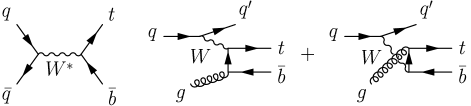
FIG. 2.: Feynman diagrams for single top quark production.

After the decay of the top quark, the particles produced in these processes are $Wb\overline{b}$ and $Wb\overline{b}q$, possibly with additional jets from QCD radiative effects. This study looks for leptonic decays of the $W$ boson, so the initial event selection requires a high-$p_{T}$ lepton, large missing transverse energy (${\hbox{$E$\kern-6.00006pt\lower-0.43057pt\hbox{/}}}_{T}$), and at least two jets. No $b$-tag is required in this study, in order to preserve signal efficiency (but if information about a tagging muon is present, it will be used).

The numbers of signal and background events expected to remain after this selection for DØ’s Run 1 ($109~{}\text{pb}^{-1}$) are as follows:

Process	$N_{\text{events}}$
$tb$	$2.1$
$tqb$	$5.1$
QCD multijet	2411
$t\overline{t}$	22.3
$Wbb$	11.4
$Wjj$ ($c$, $s$)	51.8
$Wjj$ ($g$, $u$, $d$)	1615.7
$WW$	36.9
$WZ$	5.3

As can be seen, the background is huge compared to the signal, with the dominant background sources being QCD multijet production (with a jet misidentified as a lepton) and the production of $W$ bosons with associated jets.

A crucial step in a neural network analysis is the selection of the variables used as input to the network. Adding more variables potentially increases the amount of information available to the network, but it also expands the space that must be searched during the minimization, making it more difficult to find a good minimum. In fact, with some procedures, adding variables of marginal utility can degrade the performance of a network. And while neural networks can in principle approximate any reasonable function, in practice complicated mappings may require too many hidden nodes for minimization to be practical.

FIG. 3.: Typical Feynman diagrams for the $Wjj$ and QCD backgrounds to single top quark production.

A useful observation is that the rate for a scattering process is greatest in the regions of phase space near singularities in the corresponding matrix element[boos99]. If such singularities occur in different places for signal and background, then the dependence on the corresponding variables in which the singularities occur should differ strongly between signal and background. For example, the top quark production diagrams in Fig. 2 have a singularity at $M_{t}^{2}=(p_{b}+p_{W})^{2}\rightarrow m_{t}^{2}$. In contrast, the dominant background diagrams, illustrated in Fig. 3, have singularities at

$$M_{g1,g2}^{2} =(p_{g1}+p_{g2})^{2}\rightarrow 0,$$ (7)

$$\hat{t}_{q,(g1g2)} =(p_{g1}+p_{g2}-p_{q})^{2}\rightarrow 0,$$ (8)

$$\hat{t}_{q,g1} =(p_{g1}-p_{q})^{2}\rightarrow 0,$$ (9)

$$\hat{t}_{q,g2} =(p_{g2}-p_{q})^{2}\rightarrow 0.$$ (10)

These variables, however, are defined at the parton level, and cannot be directly measured, due to effects of QCD radiation, the unobserved neutrino, and unobserved momentum that escapes down the beam pipe. In such a situation, it is better to use other variables that are related to the singular variables, but can be derived directly from the observed final state. For example, the typical $t$-channel singular variable $\hat{t}_{i,f}$ associated with the production of a light particle (or jet) $f$ can be written

$$\hat{t}_{i,f}=(p_{f}-p_{i})^{2}=-\sqrt{\hat{s}}e^{Y}p_{T}^{f}e^{-|y_{f}|},$$ (11)

where $\sqrt{\hat{s}}$ is the total invariant mass of the produced system, $Y$ is its total rapidity, and $p_{T}^{f}$ and $y_{f}$ are the transverse momentum and rapidity of the produced $f$.

From these kinds of considerations, a nominal set of input variables can be defined as:

Set 1: $$M_{j1,j2} M_{t} Y_{\text{tot}} {p_{T}}_{j1} y_{j1}$$, , , , , (12)

$$\text{${p_{T}}_{j2}$, $y_{j2}$, ${p_{T}}_{j12}$, $y_{j12}$, $\sqrt{\hat{s}}$},$$ (13)

where ${p_{T}}_{j12}$ and $y_{j12}$ are the transverse momentum and rapidity of the system formed by the two highest $p_{T}$ jets, and $Y_{\text{tot}}$ is the total rapidity of the center of mass of the initial partons, as reconstructed from the final state. The $z$-component of the momentum of the $W$ boson is found by enforcing the $M_{W}$ mass constraint in the leptonic $W$ boson decay. Distributions of some of these variables are shown in Fig. 4.

FIG. 4.: Distributions of kinematic variables for single top signal (dashed) and background (solid), either $Wjj$ (top four) or QCD (bottom two). Units are in $\text{GeV}/c^{2}$.

Figure 5 compares this set with the simpler sets:

Set 2: $${p_{T}}_{j1} {p_{T}}_{j2} H_{\text{all}} H_{T\text{all}}$$, , , ; (14)

Set 3: $${p_{T}}_{j1} {p_{T}}_{j2} H_{\text{all}} H_{T\text{all}} M_{t}$$, , , , ; (15)

where $H_{\text{all}}=\sum E_{f}$ and $H_{T\text{all}}=\sum{E_{T}}_{f}$. The comparison is made by training a neural network for each of the sets on a sample of events consisting of top quark signal plus $Wjj$ background. It is seen that the neural network built using Set 1 performs better than those using Set 2 or Set 3.

FIG. 5.: Neural network $\chi^{2}$ vs. training time, for different sets of input variables. The networks are trained on a sample consisting of the single top signal and $Wjj$ background.

Figure 5 also shows two other variations of the set of input variables. Set 4 is the same as Set 1, except that the variables $H_{\text{all}}$ and $H_{T\text{all}}$ are added. It is seen that this does worse than Set 1 — the additional variables do not add enough information to counteract the increase in the size of the minimization space. Set 5 adds to Set 1 the widths $w_{\text{jet}}$ of the two jets and the $p_{T}$ of a $b$-tagging muon (set to zero if there is no such tag). In this case, the added variables help: Set 5 has a lower $\chi^{2}$ than any of the others.

FIG. 6.: The structure of the neural networks used to reject each background. Each network has one hidden layer; the notation $(n_{1},n_{2},n_{3})$ gives the number of units in the input, hidden, and output layers of each network, respectively. The following variables are used in addition to those defined in the text. $n_{j2}$ is 1 if the event has exactly two jets and 0 otherwise; $n_{j3}$ is 1 if the event has three or more jets and 0 otherwise. The jet for which the invariant mass of the lepton, neutrino, and jet is closest to $172~{}\text{GeV}/c^{2}$ is denoted $j_{best}$; the notation $j_{all}-j_{best}$ means all jets except $j_{best}$. Also, $\Delta p_{T}(W,j_{all})=p_{T}(W)-\sum_{\text{jet}}\vec{p}_{T}^{\text{jet}}$, $\Delta M(m_{W},m_{j1},m_{j2})=|m_{W}-m(j_{1},j_{2})|/m_{W}$, and $\Delta M_{t}=|m(e,\nu,j_{best})-172|/172$.

For the final analysis, a separate network is constructed for each of the major backgrounds, as shown in Fig. 6. The networks are trained using jetnet[jetnet]; the results for each network are shown in Fig. 7. Figure 8 shows that the network output from Monte Carlo models agrees well with the data. Finally, individual cuts are made on each of the five network outputs. Figure 9 compares the results of this to a more conventional analysis. It is seen that for a given background level, the neural network analysis provides several times the signal efficiency of conventional cuts.

FIG. 7.: Outputs of each of the neural networks for single top signal (dashed) and the indicated background (solid).

FIG. 8.: A comparison of the combined output of the five networks for data (the open symbols) and a Monte Carlo model of signal and all backgrounds (the solid symbols). The individual network outputs are combined using ${1/O_{\text{tot}}}=(1/5)\sum_{i=1}^{5}1/O_{\text{NN}i}$.

FIG. 9.: Comparison of signal/background efficiencies for NN and conventional analyses. Each point represents one specific set of cuts.

IV $t\overline{t}$ Decays Into $e\mu$

The “golden” channel for observing $t\overline{t}$ decays has long been the dilepton mode $t\overline{t}\rightarrow W^{+}bW^{-}\overline{b}\rightarrow e\nu_{e}\mu\nu_{\mu}b\overline{b}$. Due to the presence of two leptons with different flavors, this channel has a very low background. However, compared to the channels in which one of the $W$ bosons decays into jets, the $e\mu$ channel has a relatively small branching ratio — about $2.5\%$, versus about $15\%$ for the $e+\text{jets}$ channel. Therefore, any new analysis techniques that can increase efficiency for identifying signal in this channel while maintaining the low background level are welcome.

This study starts from the published measurement of the $t\overline{t}$ production cross section[d0xsecprl97], which selects $e\mu$ candidates as follows:

• An electron with $E_{T}>15~{}\text{GeV}$ and $|\eta|<2.5$.

• A muon with $p_{T}>15~{}\text{GeV}/c$ and $|\eta|<1.2$.

• $\mbox{${\hbox{$E$\kern-6.00006pt\lower-0.43057pt\hbox{/}}}_{T}$}>20~{}\text{GeV}$.

• At least two jets with $E_{T}>20~{}\text{GeV}$ and $|\eta|<2.5$.

• $\Delta R_{\mu,\text{jet}}>0.5$ and $\Delta R_{e,\mu}>0.25$. ($\Delta R=\sqrt{(\Delta\phi)^{2}+(\Delta\eta)^{2}}$.)

• $H_{T}>120~{}\text{GeV}$, where $H_{T}=E_{T}^{e}+\sum_{\text{jets}}E_{T}^{\text{jet}}$.

For the present study, this selection is relaxed by removing the cut on $H_{T}$ and reducing the ${\hbox{$E$\kern-6.00006pt\lower-0.43057pt\hbox{/}}}_{T}$ and jet $E_{T}$ cuts to $15~{}\text{GeV}$. This defines the sample used as input to the neural network.

FIG. 10.: Distributions of input variables to the $\tau\tau$ neural network for signal (dashed) and $Z\rightarrow\tau\tau$ background (solid).

There are three major backgrounds to contend with: QCD jet production with jets misidentified as leptons, $Z\rightarrow\tau\tau\rightarrow e\mu$, and $WW\rightarrow e\mu$ events. A separate network is trained to separate the signal from each of the three backgrounds. Six variables are used as inputs to each of the networks, these being $E_{T}^{e}$, $E_{T}^{\text{jet}2}$, ${\hbox{$E$\kern-6.00006pt\lower-0.43057pt\hbox{/}}}_{T}$, $H_{T}^{\text{jets}}=\sum_{\text{jets}}E_{T}^{\text{jet}}$, $M_{e\mu}$, and $\Delta\phi_{e\mu}$, except for the $\tau\tau$ network, where $E_{T}^{\text{jet}1}$ replaces $E_{T}^{\text{jet}2}$. The input variables for the $\tau\tau$ network are plotted in Fig. 10. Each network has seven hidden units. The networks are trained (using jetnet) on equal numbers of $t\overline{t}$ signal and background events (2000 of each for the QCD network, and 1000 of each for the other two). The outputs of the three networks are combined, as usual, using

$$O_{\text{NN}}^{\text{comb}}={3\over{1\over O_{\text{NN}1}}+{1\over O_{\text{NN}2}}+{1\over O_{\text{NN}3}}}.$$ (16)

Distributions of this variable for signal and background are shown in Fig. 11. To define the candidate sample, a final cut of $O_{\text{NN}}^{\text{comb}}>0.88$ is imposed, which was determined by maximizing the expected relative significance, $S/\sigma_{B}$. ($\sigma_{B}$ is the uncertainty in the background estimate.)

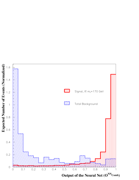
FIG. 11.: Distribution of $O_{\text{NN}}^{\text{comb}}$ for $t\overline{t}$ signal and background events.

The resulting signal efficiencies and estimated backgrounds for DØ’s Run 1 ($108~{}\text{pb}^{-1}$) are shown in Table I and Fig. 12. Compared to the standard (published) analysis, it is seen that the neural network analysis increases the signal efficiency by about $10\%$. In addition, the background is also slightly lower, although this is harder to evaluate due to the large statistical errors in the QCD background sample. Further comparison is made in Fig. 13.

	Conventional	NN
	analysis	analysis
Signal	$\epsilon\times\text{BR}$ (%)
$m_{t}=170~{}\text{GeV}/c^{2}$	$0.349\pm 0.074$	$0.386\pm 0.082$
$m_{t}=175~{}\text{GeV}/c^{2}$	$0.368\pm 0.078$	$0.402\pm 0.085$
$m_{t}=180~{}\text{GeV}/c^{2}$	$0.388\pm 0.082$	$0.420\pm 0.089$
Background	$N_{\text{expected}}$
$Z\rightarrow\tau\tau\rightarrow e\mu$	$0.10\pm 0.10$	$0.10\pm 0.07$
$WW\rightarrow e\mu$	$0.074\pm 0.020$	$0.085\pm 0.023$
$\gamma^{*}\rightarrow\tau\tau\rightarrow e\mu$	$0.006\pm 0.005$	$0.007\pm 0.006$
Fakes	$0.083\pm 0.126$	$0.048\pm 0.124$
Total	$0.26\pm 0.16$	$0.24\pm 0.15$

TABLE I.: A comparison of the results of the conventional and neural network $t\overline{t}\rightarrow e\mu$ analyses. The numbers of background events are normalized for DØ’s Run 1 ($108~{}\text{pb}^{-1}$).

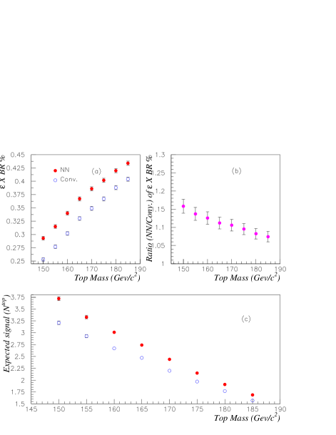
FIG. 12.: The neural network analysis compared to the standard analysis, for DØ’s Run 1. (a) Efficiency times branching ratio (%); (b) Ratio of NN analysis efficiency to standard analysis efficiency; (c) Expected number of signal events. Uncertainties displayed are statistical only; the systematic uncertainties (included in Table I) are highly correlated between the two analyses.

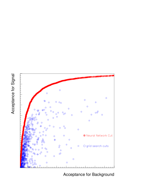
FIG. 13.: The neural network analysis compared to the standard analysis. Each point represents a different set of selection requirements.

V Conclusions

In both the analyses considered here, neural networks provide a significant improvement over conventional analysis methods. We expect that such techniques will have a prominent place in the analysis of data from the upcoming Run 2 of the Tevatron.

REFERENCES

- [1] CDF Collaboration (F. Abe et al.), Phys. Rev. Lett. 74, 2626 (1995); DØ Collaboration (S. Abachi et al.), Phys. Rev. Lett. 74, 2632 (1995).
- [2] P. Bhat, H. Prosper, and S. Snyder, Int. J. Mod. Phys. A13, 5113 (1998).
- [3] D. E. Rumelhart and J. L. McClelland, Parallel Distributed Processing, Explorations in the Microstructure of Cognition, Vol 1: Foundations (MIT Press, Boston, 1986); R. Beale and T. Jackson, Neural Computing: An Introduction (Adam Hilger, Bristol, 1990).
- [4] DØ Collaboration (B. Abbott et al.), Phys. Rev. D60, 012001 (1999); ibid, Report No. Fermilab-Pub-99/008-E (1999), hep-ex/9901023, submitted to Phys. Rev. Lett..
- [5] DØ Collaboration (B. Abbott et al.), Phys. Rev. D58, 052001 (1998); DØ Collaboration (S. Abachi et al.), Phys. Rev. Lett. 79, 1197 (1997).
- [6] K. Hornik, M. Stinchcombe, and H. White, Neural Networks 2, 359 (1989); K.-I. Funahashi, Neural Networks 2, 183 (1989).
- [7] L. Dudko, in Proceedings of the 6th International Workshop on New Computing Techniques In Physics Research (AIHENP99), Crete, Greece (Elsevier North-Holland, Amsterdam, 1999).
- [8] M. C. Smith and S. Willenbrock, Phys. Rev. D54, 6696 (1996); T. Stelzer, Z. Sullivan, and S. Willenbrock, Phys. Rev. D56, 5919 (1997); A. P. Heinson, A. S. Belyaev, and E. E. Boos, Phys. Rev. D56, 3114 (1997).
- [9] T. Tait and C.-P. Yuan, Report No. MSUHEP-71015, hep-ph/9710372 (1997).
- [10] E. Boos, L. Dudko, and T. Ohl, Report No. INP-MSU 99-4/562 (1999), hep-ph/9903215.
- [11] C. Peterson, T. Rögnvaldsson, and L. Lönnblad, Comp. Phys. Comm. 81, 185 (1994).
- [12] DØ Collaboration (S. Abachi et al.), Phys. Rev. Lett. 79, 1203 (1997).