RHEINISCH- WESTFÄLISCHE- TECHNISCHE- HOCHSCHULE- AACHEN PITHA 99/21   Juni 1999

Tests of Power Corrections to
Event Shape Distributions
from e⁺e^- Annihilation

P.A. Movilla Fernández, O. Biebel, S. Bethke


III. Physikalisches Institut, Technische Hochschule Aachen
D-52056 Aachen, Germany

 

PHYSIKALISCHE INSTITUTE RWTH AACHEN D-52056 AACHEN, GERMANY

PITHA 99/21 Juni 11, 1999

Tests of Power Corrections to
Event Shape Distributions
from e⁺e^- Annihilation

P.A. Movilla Fernández⁽¹⁾, O. Biebel⁽¹⁾, S. Bethke⁽¹⁾

A study of differential event shape distributions using e⁺e^- data at centre-of-mass energies of $\sqrt{s}$ = 35 to 183 GeV is presented. We investigated non-perturbative power corrections for the thrust, C-parameter, total and wide jet broadening observables. We observe a good description of the distributions by the combined resummed QCD calculations plus power corrections from the dispersive approach. The single non-perturbative parameter $\alpha_{0}$ is measured to be

$$\alpha_{0}({\mathrm{2~{}GeV}})=0.502\pm 0.013\mathrm{(stat.)}\ ^{+0.046}_{-0.032}\mathrm{(exp.\;syst.)}\ ^{+0.074}_{-0.053}\mathrm{(theo.\;syst.)}$$

and is found to be universal for the observables studied within the given systematic uncertainties. Using revised calculations of the power corrections for the jet broadening variables, improved consistency of the individual fit results is obtained. Agreement is also found with results extracted from the mean values of event shape distributions.

⁽¹⁾ III. Physikalisches Institut der RWTH Aachen, D-52056 Aachen, Germany contact e-mail: Pedro.Fernandez@Physik.RWTH-Aachen.DE Otmar.Biebel@Physik.RWTH-Aachen.DE

1 Introduction

The study of final states in electron-positron annihilation led to the development of numerous observables as powerful tools for the analysis of hadronic events. Improving theoretical predictions for these observables in the last years as well as the large amount of data collected by various experiments e.g. at the PETRA, PEP, LEP and SLC accelerators from $\sqrt{s}$ = 12 to 189 GeV provide precise quantitative tests of Quantum Chromodynamics (QCD). The key feature of perturbative QCD, the running of the strong coupling constant $\alpha_{s}$, has meanwhile become an indubitable experimental fact from $\mathrm{e^{+}e^{-}}$-data (see [2] and references therein), in particular due to investigation of the energy dependence of event shape data.

Precision tests of perturbative QCD from hadronic event shapes require a solid understanding of non-perturbative effects. In the context of hadronisation, non-perturbative effects are usually estimated by phenomenological hadronisation models available from Monte Carlo event generators. Alternatively, analytical approaches were pursued in the past years in order to deduce as much information as possible about hadronisation from the perturbative theory, e.g. the renormalon inspired ansatz [3] or the dispersive approach[4].

Phenomenological considerations lead to the expectation that hadronisation contributions to event shape observables evolve like reciprocal powers of the hard interaction scale $\sqrt{s}$. The investigation of power corrections therefore substantially benefits from $\mathrm{e^{+}e^{-}}$data at the lower energy region as marked by PETRA/PEP experiments at $\sqrt{s}$ = 12 to 47 GeV. Our re-analysis of $\mathrm{e^{+}e^{-}}$data collected by the JADE detector [5, 6], one of the former PETRA experiments, allowed studies of the energy evolution of QCD at combined lower and higher energies in terms of observables frequently used in the analysis of events at the highest centre-of-mass energies available at LEP. Further efforts were undertaken to make event shapes available at hadronic centre-of-mass energies below the Z pole, e.g. the analysis of radiative events recorded at LEP-1 as performed by several LEP experiments [7].

In the present paper we test power corrections to the differential distributions of event shape observables measured from re-analysed JADE data at 35 to 44 GeV and from data of the LEP/SLC experiments at 91 to 183 GeV. We focussed on two-loop predictions [8, 9] basing on the dispersive approach. For the jet broadening measures, progress was made in the understanding of non-perturbative corrections to the distributions [9], in particular the interdependence between perturbative and non-perturbative contributions. We also test a basic concept of the power corrections, the universality of the zeroth moment of the effective coupling $\alpha_{0}$ below a given infrared energy scale $\mu_{I}$.

Section 2 starts with an overview of the observables and the data used in the analysis. After some annotations to the parametrisation of the power corrections in Section 3, we present fit results basing on combined power corrections plus perturbative QCD in Section 4 and draw conclusions from our results in Section 5.

2 Event shape data

For our studies, we considered the event shape distributions of thrust, the $C$-parameter, the total and wide jet broadening, $B_{T}$ and $B_{W}$. For convenience, we list the definitions of these observables.

Thrust $T$:

The thrust value is given by the expression [10]

$$T=\max_{\vec{n}}\left(\frac{\sum_{i}|\vec{p}_{i}\cdot\vec{n}|}{\sum_{i}|\vec{p}_{i}|}\right)\ \ .$$

The thrust axis $\vec{n}_{T}$ is the vector $\vec{n}$ which maximises the expression in parentheses. It is used to divide an event into two hemispheres $H_{1}$ and $H_{2}$ by a plane through the origin and perpendicular to the thrust axis.

Jet Broadening $B$:

The jet broadening measures are calculated by [11]:

$$B_{k}=\left(\frac{\sum_{i\in H_{k}}|\vec{p}_{i}\times\vec{n}_{T}|}{2\sum_{i}|\vec{p}_{i}|}\right)$$

for each of the two hemispheres, $H_{k}$, defined above. The total jet broadening is given $B_{T}=B_{1}+B_{2}$. The wide jet broadening is defined by $B_{W}=\max(B_{1},B_{2})$.

C-parameter:

The $C$-parameter is defined as [12]

$$C=3(\lambda_{1}\lambda_{2}+\lambda_{2}\lambda_{3}+\lambda_{3}\lambda_{1})$$

where $\lambda_{\gamma}$, $\gamma=1,2,3$, are the eigenvalues of the momentum tensor

$$\Theta^{\alpha\beta}=\frac{\sum_{i}\vec{p}_{i}^{\,\alpha}\vec{p}_{i}^{\,\beta}/|\vec{p}_{i}|}{\sum_{j}|\vec{p}_{j}|}\ \ \ .$$

Experimental data for the thrust below the Z pole are provided e.g. by the experiments of the PETRA (12 to 47 GeV), PEP (29 GeV) and TRISTAN (55 to 58 GeV) colliders. For the thrust, we considered measured distributions from the PETRA experiments JADE and TASSO (total of about 50000 events), from the PEP experiments MARKII and HRS (total of about 28000 events) and from the AMY detector (about 1200 events) at TRISTAN (see Ref. [13], and [5]). For the other observables, we used experimental distributions at PETRA energies from our re-analysis of JADE data [5, 6] providing about 22000 events at 35 GeV and 6200 events at 44 GeV. The distributions used at the Z resonance stem from a measurement using several hundred thousands events for each of the four LEP experiments OPAL, ALEPH, DELPHI and L3, and of about 40000 events for the SLD experiment at SLAC [14]. We also considered measurements performed by the LEP collaborations above the Z pole [15] providing a few thousend events per experiment up to a center-of-mass energy of 183 GeV.

All distributions used in this study were corrected for the limited resolution and acceptance of the respective detectors and of the event selection criteria (for details see the referenced publications).

3 Power corrections to differential distributions

Non-perturbative effects to event shape observables arise due to the contributions of very low energetic gluons which cannot be described perturbatively because of the presence of an unphysical Landau pole in the perturbative expression of the running coupling $\alpha_{s}(M_{\mathrm{Z^{0}}})$. Within the dispersive approach [4, 8] a non-perturbative parameter

$$\alpha_{0}(\mu_{I})=\frac{1}{\mu_{I}}\int_{0}^{\mu_{I}}{\mathrm{d}}k\ \ \alpha_{s}(k)$$

is introduced to parametrize the analytic but unknown behaviour of $\alpha_{s}(\sqrt{s})$ below a certain infrared matching scale $\mu_{I}$. The technique presented in the cited papers also removes the divergent soft gluon contributions in the perturbative predictions for the observables and produces as a consequence 1/$\sqrt{s}$ corrections.

The power corrections which we used in this analysis have been calculated in Ref. [8, 9] up to two loops for the differential distributions of the event shapes considered here. The effect of hadronisation on the distribution obtained from experimental data is described by a shift of the perturbative prediction away from the kinematical 2-jet region,

$$\frac{\mathrm{d}\sigma^{\mathrm{exp}}}{\mathrm{d}{\mathcal{F}}}\left(\mathcal{F}\right)={\frac{\mathrm{d}\sigma^{\mathrm{pert}}}{\mathrm{d}{\mathcal{F}}}}\left(\mathcal{F}-\mathcal{P}D_{\mathcal{F}}\right)\;.$$ (1)

where $\mathcal{F}$ = $1-T$, $C$, $B_{T}$ and $B_{W}$, respectively. The factor $\mathcal{P}$ containing the only non-perturbative parameter $\alpha_{0}$ is the same for all observables,

$$\mathcal{P}=\frac{4C_{F}}{\pi^{2}}\mathcal{M}\frac{\mu_{I}}{\sqrt{s}}\left(\alpha_{0}(\mu_{I})-\alpha_{s}(\sqrt{s})-\beta_{0}\frac{\alpha_{s}^{2}}{2\pi}\left(\ln\frac{\sqrt{s}}{\mu_{I}}+\frac{K}{\beta_{0}}+1\right)\right)$$ (2)

where $C_{F}=4/3$. $\beta_{0}=(11C_{A}-2N_{f})/3$ stems from the QCD renormalisation group equation for $N_{C}=C_{A}$ colours and $N_{f}$ active quark flavours. $K=(67/18-\pi^{2})C_{A}-5/9N_{f}$ originates from the choice of the $\overline{\mathrm{MS}}$ renormalisation scheme. The Milan factor $\mathcal{M}$ accounts for two-loop effects. Its numerical value of 1.795 (for three active quark flavours) is given by the authors of [8] with a theoretical uncertainty of about 20% owing to missing higher order corrections. $D_{\mathcal{F}}$ is a function depending on the observable,

$$D_{\mathcal{F}}=\left\{\begin{array}[]{ll}\mathrm{2}&;{\mathcal{F}=1-T}\\[5.69054pt] \mathrm{3\pi}&;{\mathcal{F}=C}\\[5.69054pt] \frac{\textstyle 1}{\textstyle 2}\ln\frac{\textstyle 1}{\textstyle\mathcal{F}}+B_{\mathcal{F}}(\mathcal{F},\alpha_{s}(\mathcal{F}\sqrt{s}))&;{\mathcal{F}=B_{T},\,B_{W}\;.}\end{array}\right.$$ (3)

Thus a simple shift is expected for thrust and $C$-parameter, whereas for the jet broadening variables an additional squeeze of the distribution is predicted. Besides the logarithmic dependence on the value $\mathcal{F}$ of the observable, the term $B_{\mathcal{F}}$ exhibits an additional (weaker) dependence on the value of the observable and on the running coupling at the scale $\mathcal{F}\sqrt{s}$. The more complex behaviour for the jet broadening recently calculated in [9] is related to the interdependence of non-perturbative and perturbative effects which cannot be neglected for these observables. As a consequence, the term $\mathcal{P}D_{\mathcal{F}}$ leads not only to a larger shift but also to a stronger squeeze at decreasing centre-of-mass energies. The necessity of an additional non-perturbative squeeze of the jet broadening distributions was already pointed out in [16].

4 Tests of power corrections

A few experimental tests of power corrections to differential distributions have been done up to now [9, 16, 17, 18, 19]. Some studies for the new observables which were performed using LEP data only suffer from the low data statistics above the Z pole and from the lack of data at energies below the Z pole, where QCD scaling violations and energy dependent non-perturbative effects are larger. The present analysis of combined LEP and PETRA data allows a more stringent test of the $1/\sqrt{s}$ dependence of the power corrections.

4.1 Fits to the data

The standard analysis uses the entire data set described in Section 2. For the perturbative predictions, we employed combined second order [20] plus resummed [21, 22, 23, 24] QCD calculations ($\mathcal{O}(\alpha_{s}^{2})$ + NLLA). Predictions of this type take into account the dominating leading and next-to-leading logarithms to all orders in $\alpha_{s}$ in the perturbation series for the observable and therefore exhibit a weaker dependence on the QCD renormalisation scale $\mu$ = $x_{\mu}\sqrt{s}$. Since the matching procedure of the exact matrix elements and the NLLA calculations reveals some ambiguities, we apply the four different matching schemes proposed in [23], the R-, ln(R), the modified R and the modified ln(R)-matching.

For each observable, we performed simultaneous $\chi^{2}$-fits of both perturbative predictions plus power corrections which are parametrised by $\alpha_{s}(M_{\mathrm{Z^{0}}})$ and $\alpha_{0}(\mu_{I}$), respectively. $\alpha_{s}(M_{\mathrm{Z^{0}}})$ was evaluated to the appropiate energy scale $\mu$ = $x_{\mu}\sqrt{s}$ using the two-loop formula for the running coupling [25]. The errors used in the fit are the quadratic sum of statistical and experimental systematic uncertainties of the event shape distributions denoted in the references. The errors of the fit are derived from the 95% CL two-dimensional contour. The fit ranges are defined individually for each center-of-mass energy such that they, in general, include the maximum of the differential cross section located in the 2-jet-region of the distributions. In doing so we ensure to exploit the range of the distribution at each energy point as far as possible in order to constrain the theory and to consider as much data statistics as possible from the distributions, which is in particular important in regard of the scarce LEP-2 data.

Our standard result for an observable is defined by the unweighted average of the results obtained from the different $\mathcal{O}(\alpha_{s}^{2})$+NLLA-combination schemes. We fixed the renormalisation scale $x_{\mu}$ = 1 and the infrared matching scale $\mu_{I}$ = 2 GeV. The fit error assigned is the average over the individual fit errors for the matching schemes. The numeric results are listed in Table 1 for $\alpha_{s}$ and in Table 2 for $\alpha_{0}$. The fit curves for the modified ln(R)-matching and the corresponding experimental data for the thrust $1-T$, the $C$-parameter, the total and the wide jet broadening, $B_{T}$ and $B_{W}$, are shown in Figures 1, 2 and 3. Generally we observe a good agreement of the predictions with the data within the fit ranges, independent of the matching scheme used in the fit. The agreement is moderate for some distributions at $\sqrt{s}$ $\leq 35$ GeV. The $\chi^{2}/\mathrm{d.o.f.}$ of the fits (see Table 3) are between 0.93 (for $B_{T}$, mod. ln(R)-matching) and 1.34 (for $B_{W}$, R-matching). The fit quality deteriorates for the jet broadenings if the upper limit of the fit range is extended too far into the 3-jet region. The excess of the theory over the data observed here has also been noticed in other studies [26, 27, 28] where event shape distributions were corrected for hadronisation effects using Monte Carlo models. Thus these discrepancies might be due to the perturbative predictions.

The results for $\alpha_{s}(M_{\mathrm{Z^{0}}})$ obtained from the fits proved to be systematically lower than the respective results at $\sqrt{s}$ = $M_{\mathrm{Z^{0}}}$ [6, 26, 27, 28, 29] which use the same perturbative predictions but apply Monte Carlo corrections instead of power corrections. They are consistent with each other within the statistical errors in the case of thrust, $C$-parameter and the total jet broadening $B_{T}$, whereas the results obtained for $B_{W}$ is about 20% below the world average value for $\alpha_{s}(M_{\mathrm{Z^{0}}})$ [2]. This deviation is to a minor extend also present in the studies cited. Nevertheless, using the improved power corrections the values for $\alpha_{s}(M_{\mathrm{Z^{0}}})$ for $B_{T}$ and $B_{W}$ are now much more compatible with the values obtained from the other observables than is the case in our previous study [16].

The numeric results for $\alpha_{0}({\mathrm{2~{}GeV}})$ vary between 0.437 for the $C$-parameter and 0.685 for $B_{W}$. The high value for $B_{W}$ is supposed to be partially related to the systematically lower values of $\alpha_{s}$, since the two fit parameters are anticorrelated (see Table 3 for the correlations coefficients).

From the experimental point of view, there is a lucid explanation for the deviations of the $\alpha_{s}$ results based on the power corrections from those based on Monte Carlo corrections [16]. We realised in our studies that the latter induce a stronger squeeze to all distributions than the power corrections which for instance predict merely a shift for the thrust and the $C$-paramter without any presence of a squeeze. Although the situation was a little remedied for the jet broadenings $B$ due to the factor ln $1/B$ appearing in Equation (3), the extend of the squeezing remains below the expectation of hadronisation models. As a consequence, the two-parameter fit favours systematically smaller values for $\alpha_{s}$ in order to make the predicted shape more peaked in the 2 jet region of the distribution (thus causing a squeeze) and hence chooses high values for $\alpha_{0}$ in order to compensate the resulting shift of the distribution towards the 2-jet-region, as is in particular the case for the jet broadenings.

4.2 Systematic uncertainties

In order to scrutinize the universality of the non-perturbative parameter $\alpha_{0}$  we also studied the impact of systematic uncertainties to our final results. Theoretical uncertainties from perturbation theory were assessed by considering the different matching schemes and by varying $x_{\mu}$ from 0.5 to 2.0. For the further systematic checks, we took the modified ln(R)-matching scheme as a reference since it turned out that most of the relative changes of $\alpha_{s}$ and $\alpha_{0}$ are not significantly affected by the choice of the matching scheme. Uncertainties due to the parametrisation of the power corrections are associated with the arbitrariness of the choice of the value of $\mu_{I}$ which has been varied by $\pm$ 1 GeV. Furthermore the Milan factor $\mathcal{M}$ was varied within the quoted uncertainty of 20%. No error contribution from the infrared matching scale is assigned to $\alpha_{0}(\mu_{I}$).

The signed values in Tables 1 and 2 indicate the direction in which $\alpha_{s}(M_{\mathrm{Z^{0}}})$ and $\alpha_{0}$ changed with respect to the standard analysis. It turns out that the non-perturbative uncertainties for $\alpha_{s}(M_{\mathrm{Z^{0}}})$ are negligible for each observable. This is in accordance with the expectation since $\alpha_{s}$ is mainly constrained by the perturbative prediction and not by the non-perturbative shift $\propto\mu_{I}\mathcal{M}(\alpha_{0}-\alpha_{s}+\mathcal{O}(\alpha_{s}^{2}))$. On the other hand, the strong dependence of $\alpha_{0}$ on $\mathcal{M}$ is due to the obvious anticorrelation. In regard to the remarks made in Section 4.1 it is noticable that the value for $\alpha_{0}$ from $B_{W}$ is affected with the largest non-perturbative error.

We also examined the dependence of the results from the input data taken for the fits which is for brevity denoted as “experimental uncertainty”. Since the statistical weight of the event shape distributions at $\sqrt{s}$ = 91 GeV is dominant in the fits, the analysis was repeated using the data from each LEP/SLC experiment seperately as representative for $\sqrt{s}$ = 91 GeV. Each deviation from the standard result was added in quadrature. In addition, we performed a measurement omiting the 91 GeV data. The larger of the two latter deviations were incorporated in the experimental error. Furthermore, an analysis was performed using seperately either event shape data below the Z pole or data at $\sqrt{s}$ $\geq M_{Z^{0}}$. This checks also for higher order non-perturbative contributions $\propto(1/\sqrt{s})^{2}$ to the power corrections.

A further source of experimental uncertainty comes from the choice of the fit range. We quantified it by varying the lower and the upper edge of the fit range of all distributions likewise in both directions by an amount approximately corresponding to the respective bin of the JADE distribution at 35 GeV. The fit range of a distribution was expanded into the 2-jet region as far as the $\chi^{2}$ of the extreme bin did not contribute substantially to the total $\chi^{2}$ of the distribution. For each edge, we took the larger deviation from the standard result as error.

In general, the experimental errors are more moderate than the theoretical uncertainties. We realise major variations of $\alpha_{s}(M_{\mathrm{Z^{0}}})$ from $B_{T}$ and $B_{W}$ when considering only PETRA data in the fits. The larger dependence of the results on the lower edge of the fit range of the thrust distribution may be partially ascribed to the contributions of the lower energy data down to 14 GeV at which mass effects become important.

All errors are treated as asymmetric uncertainties on $\alpha_{s}(M_{\mathrm{Z^{0}}})$ and $\alpha_{0}(\mu_{I}$), respectively. The total errors are quoted as the quadratic sum of the individual uncertainties, thus disregarding possible correlations between them. They are also given in Table 1 and 2 for $\alpha_{s}$ and $\alpha_{0}$, respectively.

4.3 Combination of individual results

The individual results for the four event shape observables were combined to a single value for $\alpha_{s}(M_{\mathrm{Z^{0}}})$ and $\alpha_{0}({\mathrm{2~{}GeV}})$, respectively, following the procedure described in [5]. This procedure accounts for correlations of the systematic errors. A weighted average of the individual results was calculated with the square of the reciprocal total errors used as the weight. For each of the systematic checks, the mean values for $\alpha_{s}(M_{\mathrm{Z^{0}}})$ and $\alpha_{0}({\mathrm{2~{}GeV}})$ from all considered observables were determined. Any deviation from the weighted average of the main result was taken as a systematic uncertainty.

With this procedure, we obtained as final result for $\alpha_{0}({\mathrm{2~{}GeV}})$

$$\alpha_{0}({\mathrm{2~{}GeV}})=0.502\pm 0.013\mathrm{(stat.)}\ ^{+0.046}_{-0.032}\mathrm{(exp.\;syst.)}\ ^{+0.074}_{-0.053}\mathrm{(theo.\;syst.)}$$

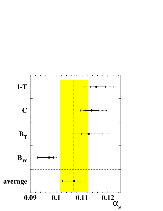
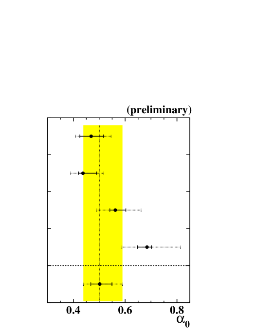
Figure 4: Results for $\alpha_{s}(M_{\mathrm{Z^{0}}})$ and $\alpha_{0}({\mathrm{2~{}GeV}})$ from fits of power corrections to the event shape distributions of thrust $T$, $C$-parameter, total and wide jet broadening, $B_{T}$ and $B_{W}$, respectively. The experimental and statistical uncertainties are represented by the solid error bars. The dashed error bars show the total error including theoretical uncertainties from the resummed QCD and the power corrections. The shaded band shows the one standard deviation around the weighted average.

where the error is dominated by non-perturbative uncertainties. Figure 4 illustrates that the individual results are compatible with the weighted mean within the total errors. We consider this result as a confirmation of the predicted universality of the non-perturbative parameter $\alpha_{0}$.

Employing the same procedure for $\alpha_{s}(M_{\mathrm{Z^{0}}})$, we obtain

$$\alpha_{s}(M_{\mathrm{Z^{0}}})=0.1068\pm 0.0011\mathrm{(stat.)}\ ^{+0.0033}_{-0.0043}\mathrm{(exp.\;syst.)}^{+0.0043}_{-0.0029}\mathrm{(theo.\;syst.)}\;.$$

This small value compared to the world average [2] is due to the $\alpha_{s}$ from $B_{W}$ which is substantially below the $\alpha_{s}$ from $T$, $C$-parameter $B_{T}$ (see Figure 4).

If $B_{W}$ is omited, the final value is $\alpha_{s}(M_{\mathrm{Z^{0}}})=0.1141$ $\pm 0.0012\mathrm{(stat.)}$ ${}^{+0.0034}_{-0.0024}\mathrm{(exp.\;syst.)}$ ${}^{+0.0055}_{-0.0041}\mathrm{(theo.\;syst.)}$ which is in good agreement with the world average value [2]. In this case, the result for $\alpha_{0}$ does insignificantly change to $\alpha_{0}({\mathrm{2~{}GeV}})=0.478$ $\pm 0.013\mathrm{(stat.)}$ ${}^{+0.047}_{-0.020}\mathrm{(exp.\;syst.)}$ ${}^{+0.067}_{-0.048}\mathrm{(theo.\;syst.)}$.

5 Summary and conclusions

The analytic treatment of non-perturbative effects to hadronic event shapes based on power corrections were examined. We tested predictions [8, 9] for the differential distributions of thrust, $C$-parameter, total and wide jet broadening, $B_{T}$ and $B_{W}$, respectively. For this test, a large amount of event shape data collected by several experiments over a huge range of $\mathrm{e^{+}e^{-}}$annihilation energies from $\sqrt{s}$ = 14 to 183 GeV was considered. For the $C$-parameter, $B_{T}$ and $B_{W}$, differential distributions below the Z pole are provided by our re-analysis of $\mathrm{e^{+}e^{-}}$data of the JADE experiment [5, 6] at $\sqrt{s}$ = 35 and 44 GeV.

A simultaneous two-parameter fit of the combined power corrections plus perturbative QCD-predictions ($\mathcal{O}(\alpha_{s}^{2})$+NLLA) was performed for both the strong coupling $\alpha_{s}(M_{\mathrm{Z^{0}}})$ and the non-perturbative parameter $\alpha_{0}(\mu_{I}$). The good quality of the fits with $\chi^{2}/\mathrm{d.o.f.}$ around 1.0 for each observable supports the predicted $1/\sqrt{s}$-evolution of the power corrections. The results for $\alpha_{s}(M_{\mathrm{Z^{0}}})$ and $\alpha_{0}({\mathrm{2~{}GeV}})$ are more consistent with each other due to the improved predictions of power corrections to the jet broadening variables [9]. Nevertheless we still observe a large deviation of the results obtained from $B_{W}$ from those extracted from the other observables. We suspect it to be partially due to the resummed predictions for this observable. The individual results for $\alpha_{s}$ from all observables (Table 1) are systematically smaller than the respective results in [6, 26, 27, 28, 29], the latter employing hadronisation models for the correction of non-perturbative effects. This observation is presumably related to the different extends of the non-perturbative squeeze of the distributions predicted by the both ansatzes. We obtain as combined result

$$\alpha_{s}(M_{\mathrm{Z^{0}}})=0.107\ ^{+0.006}_{-0.005}\;.$$

It should be noted that $\alpha_{s}$ from the wide jet broadening $B_{W}$ is rather small compared with the $\alpha_{s}$ from the other observables. The combined value for $\alpha_{s}(M_{\mathrm{Z^{0}}})$ derived when omiting the results for $B_{W}$ is $\alpha_{s}(M_{\mathrm{Z^{0}}})=0.114\ ^{+0.007}_{-0.005}(\mathrm{tot.})$, in agreement with direct measurements at the Z resonance [26, 27, 28, 29] and with the world average value of $\alpha_{s}^{w.a.}(M_{\mathrm{Z^{0}}})=0.119\pm 0.004$.

The combination of the individual results for $\alpha_{0}$ from all observables considered yields as final result for the coupling moment

$$\alpha_{0}(2~{}\mathrm{GeV})=0.50\ ^{+0.09}_{-0.06}$$

where the error is dominated by theoretical uncertainties defined in Section 4.2. Since this value is representative for the individual results within the errors defined, we consider this as a confirmation of the universality of $\alpha_{0}$ as predicted within the dispersive approach [8] of power corrections. Nevertheless, the results yielded from $B_{T}$ and $B_{W}$ indicate that higher orders may contribute significantly to the non-perturbative corrections for the jet broadenings.

We point out that the average value for $\alpha_{0}({\mathrm{2~{}GeV}})$ derived from the differential event shape distributions is in good agreement with the result of $\alpha_{0}({\mathrm{2~{}GeV}})=0.47\ ^{+0.06}_{-0.04}$ provided by our previous study [6] of power corrections to the mean values of event shapes.

Tables

	$\mathbf{1-T}$	$\mathbf{C}$	$\mathbf{B_{T}}$	$\mathbf{B_{W}}$
$\mathbf{\alpha_{s}(M_{\mathrm{Z^{0}}})}$	0.1156	0.1137	0.1125	0.0973
Exp. stat.	$\pm$ 0.0011	$\pm$ 0.0011	$\pm$ 0.0014	$\pm$ 0.0009
pQCD	$\stackrel{{\scriptstyle\textstyle\mathbf{+0.0055}}}{{\textstyle\mathbf{-0.0043}}}$	$\stackrel{{\scriptstyle\textstyle\mathbf{+0.0051}}}{{\textstyle\mathbf{-0.0036}}}$	$\stackrel{{\scriptstyle\textstyle\mathbf{+0.0063}}}{{\textstyle\mathbf{-0.0054}}}$	$\stackrel{{\scriptstyle\textstyle\mathbf{+0.0026}}}{{\textstyle\mathbf{-0.0015}}}$
Pow. corr.	$\stackrel{{\scriptstyle\textstyle\mathbf{+0.0007}}}{{\textstyle\mathbf{-0.0006}}}$	$\stackrel{{\scriptstyle\textstyle\mathbf{+0.0000}}}{{\textstyle\mathbf{-0.0001}}}$	$\stackrel{{\scriptstyle\textstyle\mathbf{+0.0002}}}{{\textstyle\mathbf{-0.0003}}}$	$\stackrel{{\scriptstyle\textstyle\mathbf{+0.0000}}}{{\textstyle\mathbf{-0.0000}}}$
Exp. syst.	$\stackrel{{\scriptstyle\textstyle\mathbf{+0.0034}}}{{\textstyle\mathbf{-0.0021}}}$	$\stackrel{{\scriptstyle\textstyle\mathbf{+0.0026}}}{{\textstyle\mathbf{-0.0022}}}$	$\stackrel{{\scriptstyle\textstyle\mathbf{+0.0050}}}{{\textstyle\mathbf{-0.0023}}}$	$\stackrel{{\scriptstyle\textstyle\mathbf{+0.0015}}}{{\textstyle\mathbf{-0.0043}}}$
Total	$\stackrel{{\scriptstyle\textstyle\mathbf{+0.0066}}}{{\textstyle\mathbf{-0.0049}}}$	$\stackrel{{\scriptstyle\textstyle\mathbf{+0.0058}}}{{\textstyle\mathbf{-0.0044}}}$	$\stackrel{{\scriptstyle\textstyle\mathbf{+0.0082}}}{{\textstyle\mathbf{-0.0061}}}$	$\stackrel{{\scriptstyle\textstyle\mathbf{+0.0031}}}{{\textstyle\mathbf{-0.0046}}}$
ln(R)	$-0.0002$	$-0.0001$	$-0.0015$	$<0.0001$
ln(R) mod.	$+0.0008$	$+0.0011$	$+0.0029$	$+0.0013$
R	$-0.0010$	$-0.0005$	$-0.0032$	$-0.0010$
R mod.	$+0.0004$	$-0.0005$	$+0.0018$	$-0.0003$
$x_{\mu}=0.5$	$-0.0041$	$-0.0035$	$-0.0041$	$-0.0010$
$x_{\mu}=2.0$	$+0.0055$	$+0.0050$	$+0.0053$	$+0.0022$
${\cal M}-20\%$	$+0.0003$	$<0.0001$	$+0.0002$	$<0.0001$
${\cal M}+20\%$	$-0.0003$	$<0.0001$	$-0.0001$	$<0.0001$
91 GeV = OPAL	$-0.0006$	$+0.0004$	$-0.0011$	$-0.0023$
91 GeV = ALEPH	$-0.0001$	$-0.0004$	—	—
91 GeV = DELPHI	$-0.0001$	$+0.0005$	$+0.0009$	$+0.0011$
91 GeV = L3	$-0.0010$	$-0.0011$	—	—
91 GeV = SLD	$-0.0014$	$-0.0017$	$+0.0004$	$-0.0008$
$\sqrt{s}\neq 91$ GeV	$-0.0003$	$-0.0004$	$+0.0020$	$-0.0012$
$\sqrt{s}\geq 91$ GeV	$+0.0019$	$<0.0001$	$+0.0002$	$+0.0001$
$\sqrt{s}<91$ GeV	$+0.0007$	$+0.0024$	$+0.0046$	$-0.0035$
fit range	$\stackrel{{\scriptstyle\textstyle+0.0027}}{{\textstyle-0.0010}}$	$\stackrel{{\scriptstyle\textstyle+0.0004}}{{\textstyle-0.0009}}$	$\stackrel{{\scriptstyle\textstyle+0.0006}}{{\textstyle-0.0021}}$	$\stackrel{{\scriptstyle\textstyle+0.0010}}{{\textstyle-0.0005}}$

Table 1: Values of $\alpha_{s}(M_{\mathrm{Z^{0}}})$ derived using combined power corrections plus resummed QCD predictions to the event shape distributions of trust $T$, $C$-parameter, total and wide jet broadening $B_{T}$ and $B_{W}$. The standard result for each variable is defined as the unweighted average of the results from the different matching schemes (ln(R), ln(R) mod., R, R mod.) using $x_{\mu}=1$ and $\mu_{I}=2$ GeV and considering the entire data set. In addition, the statistical and systematic uncertainties are given. Signed values indicate the direction in which $\alpha_{s}(M_{\mathrm{Z^{0}}})$ changed with respect to the standard analysis. Theoretical uncertainties are given by the matching scheme ambiguity, the choice of $x_{\mu}$ and $\mu_{I}$ and the uncertainty of the Milan factor ${\cal M}$. Experimental uncertainties are taken into account by varying the input data of the fit (see text). All errors are treated as asymmetric uncertainties on $\alpha_{s}(M_{\mathrm{Z^{0}}})$.

	$\mathbf{1-T}$	$\mathbf{C}$	$\mathbf{B_{T}}$	$\mathbf{B_{W}}$
$\mathbf{\alpha_{0}}$	0.469	0.437	0.562	0.685
Exp. stat.	$\pm$ 0.011	$\pm$ 0.010	$\pm$ 0.017	$\pm$ 0.014
pQCD	$\stackrel{{\scriptstyle\textstyle\mathbf{+0.009}}}{{\textstyle\mathbf{-0.009}}}$	$\stackrel{{\scriptstyle\textstyle+\mathbf{0.026}}}{{\textstyle\mathbf{-0.027}}}$	$\stackrel{{\scriptstyle\textstyle\mathbf{+0.041}}}{{\textstyle\mathbf{-0.041}}}$	$\stackrel{{\scriptstyle\textstyle\mathbf{+0.029}}}{{\textstyle\mathbf{-0.033}}}$
Pow. corr.	$\stackrel{{\scriptstyle\textstyle\mathbf{+0.060}}}{{\textstyle\mathbf{-0.040}}}$	$\stackrel{{\scriptstyle\textstyle\mathbf{+0.055}}}{{\textstyle\mathbf{-0.037}}}$	$\stackrel{{\scriptstyle\textstyle\mathbf{+0.081}}}{{\textstyle\mathbf{-0.054}}}$	$\stackrel{{\scriptstyle\textstyle\mathbf{+0.125}}}{{\textstyle\mathbf{-0.084}}}$
Exp. syst.	$\stackrel{{\scriptstyle\textstyle\mathbf{+0.047}}}{{\textstyle\mathbf{-0.042}}}$	$\stackrel{{\scriptstyle\textstyle\mathbf{+0.052}}}{{\textstyle\mathbf{-0.013}}}$	$\stackrel{{\scriptstyle\textstyle\mathbf{+0.037}}}{{\textstyle\mathbf{-0.012}}}$	$\stackrel{{\scriptstyle\textstyle\mathbf{+0.011}}}{{\textstyle\mathbf{-0.034}}}$
Total	$\stackrel{{\scriptstyle\textstyle\mathbf{+0.077}}}{{\textstyle\mathbf{-0.060}}}$	$\stackrel{{\scriptstyle\textstyle\mathbf{+0.081}}}{{\textstyle\mathbf{-0.049}}}$	$\stackrel{{\scriptstyle\textstyle\mathbf{+0.099}}}{{\textstyle\mathbf{-0.071}}}$	$\stackrel{{\scriptstyle\textstyle\mathbf{+0.130}}}{{\textstyle\mathbf{-0.097}}}$
ln(R)	$+0.003$	$+0.019$	$+0.023$	$+0.012$
ln(R) mod.	$-0.005$	$-0.015$	$-0.025$	$-0.019$
R	$+0.007$	$+0.016$	$+0.033$	$+0.021$
R mod.	$-0.005$	$-0.020$	$-0.032$	$-0.014$
$x_{\mu}=0.5$	$-0.006$	$-0.012$	$-0.008$	$-0.023$
$x_{\mu}=2.0$	$+0.005$	$+0.008$	$+0.007$	$+0.017$
${\cal M}-20\%$	$+0.060$	$+0.055$	$+0.081$	$+0.125$
${\cal M}+20\%$	$-0.040$	$-0.037$	$-0.054$	$-0.084$
91 GeV = OPAL	$+0.018$	$+0.027$	$+0.022$	$+0.010$
91 GeV = ALEPH	$+0.018$	$+0.020$	—	—
91 GeV = DELPHI	$<0.001$	$-0.013$	$-0.010$	$-0.017$
91 GeV = L3	$+0.021$	$+0.024$	—	—
91 GeV = SLD	$+0.020$	$+0.025$	$+0.006$	$-0.024$
$\sqrt{s}\neq 91$ GeV	$+0.020$	$+0.021$	$+0.008$	$-0.021$
$\sqrt{s}\geq 91$ GeV	$-0.029$	$-0.003$	$-0.005$	$+0.005$
$\sqrt{s}<91$ GeV	$+0.020$	$+0.019$	$+0.004$	$+0.001$
fit range	$\stackrel{{\scriptstyle\textstyle+0.018}}{{\textstyle-0.031}}$	$\stackrel{{\scriptstyle\textstyle+0.008}}{{\textstyle-0.001}}$	$\stackrel{{\scriptstyle\textstyle+0.030}}{{\textstyle-0.005}}$	$\stackrel{{\scriptstyle\textstyle+0.002}}{{\textstyle-0.017}}$

Table 2: Values of $\alpha_{0}(\mu_{I}$) derived using combined power corrections plus resummed QCD predictions to the event shape distributions of trust $T$, $C$-parameter, total and wide jet broadening $B_{T}$ and $B_{W}$. The standard result for each variable is defined as the average of the results from the different matching schemes (ln(R), ln(R) mod., R, R mod.) using $x_{\mu}$ = 1 and $\mu_{I}$ =2 GeV and considering the entire data set. In addition, the statistical and systematic uncertainties are given. Signed values indicate the direction in which $\alpha_{s}(M_{\mathrm{Z^{0}}})$ changed with respect to the standard analysis. Theoretical uncertainties are given by the matching scheme ambiguity, the choice of $x_{\mu}$ and the uncertainty of the Milan factor ${\cal M}$. Experimental uncertainties are taken into account by varying the input data of the fit. All errors are treated as asymmetric uncertainties on $\alpha_{0}$.

	$\mathbf{1-T}$	$\mathbf{C}$	$\mathbf{B_{T}}$	$\mathbf{B_{W}}$
ln(R)	283.7/277	162.9/170	161.0/171	162.1/132
corr.	-76%	-60%	-77%	-57%
ln(R) mod.	341.8/277	185.9/170	158.2/171	133.0/132
corr.	-78%	-72%	-84%	-63%
R	269.7/277	155.9/163	179.5/171	177.1/132
corr.	-75%	-61%	-76%	-56%
R mod.	329.0/277	171.4/163	160.7/171	139.3/132
corr.	-78%	-75%	-84%	-64%

Table 3: Values for $\chi^{2}/\mathrm{d.o.f.}$ from the ($\alpha_{s}$,$\alpha_{0}$)-fits of combined power corrections plus resummed QCD predictions using the for different matching schemes. Also shown are the correlation coefficients of the fits. In the case of some $C$-parameter distributions, the fit ranges for the R- and the modified R-matching had to be chosen slighty different from those of the ln(R)- and the modified ln(R) matching in order to ensure the convergence of the fit.

Figures

Figure 1: Scaled distributions for $1-T$ measured by several experiments at $\sqrt{s}=14$ to $183$ GeV. The error bars indicate the statistical and experimental errors of the data points. The curves are the result of the simultaneous global ($\alpha_{s}$,$\alpha_{0}$)-fit using resummed QCD predictions with the modified ln(R)-matching plus power corrections. The fit ranges which are indicated by the solid lines are chosen individually for each center-of-mass energy.

Figure 2: Scaled distributions for the $C$-parameter measured by several experiments at $\sqrt{s}=35$ to $183$ GeV. The error bars indicate the statistical and experimental errors of the data points. The curves are the result of the simultaneous global ($\alpha_{s}$,$\alpha_{0}$)-fit using resummed QCD predictions with the modified ln(R)-matching plus power corrections. The fit ranges which are indicated by the solid lines are chosen individually for each center-of-mass energy.

       

Figure 3: Scaled distributions for $B_{T}$ (left) and $B_{W}$ (right) measured by several experiments at $\sqrt{s}=35$ to $183$ GeV. The error bars indicate the statistical experimental errors of the data points. The curves are the result of the simultaneous global ($\alpha_{s}$,$\alpha_{0}$)-fit using resummed QCD predictions with the modified ln(R)-matching plus power corrections which include the revised power corrections to jet broadening observables[9]. The fit ranges which are indicated by the solid lines are chosen individually for each center-of-mass energy.

References

- [1]
- [2] S. Bethke: proceedings of the IVth International Symposium on Radiative Corrections, Barcelona, Spain, September 9-12 (1998), PITHA 98/43, hep-ex/9812026.
- [3] A.H. Mueller: in QCD — 20 Years Later, vol. 1, ed. P.M. Zerwas and H.A. Kastrup, World Scientific, Singapore, 1993.
-
[4]
Yu.L. Dokshitzer, B.R. Webber: Phys. Lett. B352 (1995) 451;
B.R. Webber: proceedings of the Workshop on Deep Inelastic Scattering and QCD (DIS 95), Paris, France, 24-28 Apr, 1995, ed. J.F. Laporte and Y. Sirois; Cavendish-HEP-95/11; hep-ph/9510283. - [5] P.A. Movilla Fernández, O. Biebel, S. Bethke, S. Kluth, P. Pfeifenschneider and the JADE collaboration: Eur. Phys. J. C1 (1998) 461, hep-ex/9708034.
- [6] O. Biebel, P.A. Movilla Fernández, S. Bethke and the JADE Collaboration: C-Parameter and Jet Broadening at PETRA Energies, hep-ex/9803009, submitted to Phys. Lett. B.
-
[7]
L3 Coll., M. Acciarri et al.: Phys. Lett. B411 (1997) 339;
L3 Coll.: L3 Note 2304 (1998);
DELPHI Coll., J. Drees et al.: DELPHI 99-19 CONF 219 (1999). -
[8]
Yu.L. Dokshitzer, A. Lucenti, G. Marchesini, G.P. Salam,
Universality of corrections to jet-shape
observables rescued,
Nucl. Phys. B511 (1998) 396;
IFUM-573-FT;
Yu.L. Dokshitzer, A. Lucenti, G. Marchesini, G.P. Salam: On the universality of the Milan factor for power corrections to jet shapes, J. High Energy Phys. JHEP 05 (1998) 003, IFUM-601-FT, hep-ph/9802381;
G.P. Salam: The Milan factor for jet-shape observables, IFUM-623-FT, hep-ph/9805323. - [9] Yu.L. Dokshitzer, G. Marchesini, G.P. Salam: Revisiting non-perturbative effects in the jet broadenings, Bicocca-FT-98-01, hep-ph/9812487.
-
[10]
S. Brandt et al.: Phys. Lett. B12 (1964) 57;
E. Fahri: Phys. Rev. Lett. 39 (1977) 1587. - [11] S. Catani, G. Turnock, B.R. Webber: Phys. Lett. B295 (1992) 269.
-
[12]
G. Parisi: Phys. Lett. B74 (1978) 65;
J.F. Donoghue, F.E. Low, S.Y. Pi: Phys. Rev. D20 (1979) 2759. -
[13]
AMY Coll., Y.K. Li et al.: Phys. Rev. D41 (1990) 2675;
HRS Coll., D. Bender et al.: Phys. Rev. D31 (1985) 1;
MarkII Coll., A. Petersen et al.: Phys. Rev. D37 (1988) 1;
TASSO Coll., W. Braunschweig et al.: Z. Phys. C41 (1988) 359;
TASSO Coll., W. Braunschweig zet al.: Z. Phys. C47 (1990) 187. -
[14]
ALEPH Coll., D. Buskulic et al.: Z. Phys. C55 (1992) 209;
DELPHI Coll., P. Abreu et al.: Z. Phys. C73 (1996) 11;
L3 Coll., B. Adeva et al.: Z. Phys. C55 (1992) 39;
OPAL Coll., P.D. Acton et al.: Z. Phys. C55 (1992) 1;
OPAL Coll., P.D. Acton et al.: Z. Phys. C59 (1993) 1;
SLD Coll., K. Abe et al.: Phys. Rev. D51 (1995) 962. -
[15]
ALEPH Coll., D. Buskulic et al.: Z. Phys. C73 (1997) 409;
ALEPH Coll.: “QCD studies with e+e- annihilation data from to GeV”, contributed paper to ICHEP98 #945 (1998);
DELPHI Coll., P. Abreu et al.: Z. Phys. C73 (1997) 229;
DELPHI Coll.: “qcd Results from the delphi Measurements at GeV and GeV”, contributed paper to HEP97 #544 (1997);
DELPHI Coll.: “ from delphi Measurements at lep 2”, contributed paper to ICHEP98 #137 (1998);
L3 Coll., M. Acciarri et al.: Phys. Lett. B371 (1996) 137;
L3 Coll., M. Acciarri et al.: Phys. Lett. B404 (1997) 390;
Su. Banerjee, Sw. Banerjee, D. Duchesneau and S. Sarkar: “QCD-Results at GeV and GeV”, L3 note 2059, contributed to EPS97 and Lepton-Photon 97 # 498, LP-046 (1997);
L3 Coll., M. Acciarri et al.: Phys. Lett. B411 (1997) 339;
L3 Coll., M. Acciarri et al.: Phys. Lett. B444 (1998) 569;
OPAL Coll., G. Alexander et al.: Z. Phys. C72 (1996) 191;
OPAL Coll., K. Ackerstaff et al.: Z. Phys. C75 (1997) 193;
OPAL Coll.: “QCD studies with e+e- annihilation data at GeV”, contributed paper to ICHEP98 #304 (1998). - [16] P.A. Movilla Fernández: Nucl.Phys. B (Proc.Suppl.) 74 (1999) 384; proceedings of the QCD Euroconference 98, Montpellier, France, July 2-8, 1998; PITHA 98/24, hep-ex/9808005.
- [17] Yu.L. Dokshitzer, B.R. Webber: Phys. Lett. B404 (1997) 321.
- [18] D. Wicke: Nucl. Phys. B (Proc.Suppl.) 64 (1998) 27; proceedings of the QCD Euroconference 97, Montpellier, France, July 3-9, 1997.
-
[19]
ALEPH Coll.: Power Law Corrections to Hadronic Event-Shape Variables
in e+e- Annihilation, contributed paper
to HEP97 and Lepton-Photon 97 # 610, LP258 (1997);
ALEPH Coll.: Measurements of with e+e- annihilation data from 91 to 183 GeV, contributed paper to ICHEP98 #940 (1998). - [20] R.K. Ellis, D.A. Ross, A.E. Terrano: Nucl. Phys. B178 (1981) 421.
- [21] S. Catani, B.R. Webber: Phys. Lett. B427 (1998) 377.
- [22] Yu.L. Dokshitzer, A. Lucenti, G. Marchesini, G.P. Salam: J. High Energy Phys. JHEP 01 (1998) 011.
- [23] S. Catani, L. Trentadue, G. Turnock and B.R. Webber: Nucl. Phys. B407 (1993) 3.
- [24] G. Dissertori, M. Schmelling: Phys. Lett. B361 (1995) 167.
- [25] Particle Data Group, R.M. Barnett et al.: Phys. Rev. D54 (1996) 1.
- [26] OPAL Coll., P.D. Acton et al.: Z. Phys. C59 (1993) 1.
- [27] DELPHI Coll., P. Abreu et al.: Z. Phys. C59 (1993) 21.
- [28] SLD Coll., K. Abe et al.: Phys. Rev D51 (1995) 962.
- [29] ALEPH Coll., D. Decamp et al.: Phys. Lett. B284 (1992) 408.