Extraction of the Width of the $W$ Boson from Measurements of $\sigma(p\overline{p}\rightarrow W+X)\cdot B(W\rightarrow e\nu)$ and $\sigma(p\overline{p}\rightarrow Z+X)\cdot B(Z\rightarrow ee)$ and their Ratio

Abstract

We report on measurements of inclusive cross sections times branching fractions into electrons for $W$ and $Z$ bosons produced in $p\overline{p}$ collisions at $\sqrt{s}$ = 1.8 TeV. From an integrated luminosity of 84.5 pb^-1 recorded in 1994–1995 using the DØ detector at the Fermilab Tevatron, we determine $\sigma(p\overline{p}\rightarrow W+X)\cdot B(W\rightarrow e\nu)$= 2310 $\pm$ 10 (stat) $\pm$ 50 (syst) $\pm$ 100 (lum) pb and $\sigma(p\overline{p}\rightarrow Z+X)\cdot B(Z\rightarrow ee)$= 221 $\pm$ 3 (stat) $\pm$ 4 (syst) $\pm$ 10 (lum) pb. From these, we derive $\sigma(p\overline{p}\rightarrow W+X)\cdot B(W\rightarrow e\nu)/\sigma(p\overline{p}\rightarrow Z+X)\cdot B(Z\rightarrow ee)$ = 10.43 $\pm$ 0.15 (stat) $\pm$ 0.20 (syst) $\pm$ 0.10 (NLO), $B(W\rightarrow e\nu)$ = 0.1066 $\pm$ 0.0015 (stat) $\pm$ 0.0021 (syst) $\pm$ 0.0011 (theory) $\pm$ 0.0011 (NLO), and $\Gamma_{W}$ = 2.130 $\pm$ 0.030 (stat) $\pm$ 0.041 (syst) $\pm$ 0.022 (theory) $\pm$ 0.021 (NLO) GeV. We use the latter to set a 95% confidence level upper limit on the partial decay width of the $W$ boson into non-standard model final states, $\Gamma_{W}^{inv}$, of 0.168 GeV. Combining these results with those from the 1992–1993 data gives $\sigma(p\overline{p}\rightarrow W+X)\cdot B(W\rightarrow e\nu)/\sigma(p\overline{p}\rightarrow Z+X)\cdot B(Z\rightarrow ee)$ = 10.54 $\pm$ 0.24, $\Gamma_{W}$ = 2.107 $\pm$ 0.054 GeV, and a 95% C.L. upper limit on $\Gamma_{W}^{inv}$ of 0.132 GeV. Using a sample with a luminosity of 505 nb^-1 taken at $\sqrt{s}$ = 630 GeV, we measure $\sigma(p\overline{p}\rightarrow W+X)\cdot B(W\rightarrow e\nu)$ = 658 $\pm$ 67 pb.

I Introduction

Since their discovery in 1983 [1], comparison of the properties of $W$ and $Z$ bosons to predictions of the standard model has been a subject of intense study [2, 3, 4, 5, 6, 7]. One such property is the $W$ boson width. Within the standard model, the $W$ boson decays into quark or lepton electroweak doublets. To lowest order, the partial decay width of the $W$ boson into massless fermions $f\bar{f^{\prime}}$ can be written as

$$\Gamma_{W\rightarrow f\bar{f^{\prime}}}=|V_{f\bar{f^{\prime}}}|^{2}N_{C}(G_{F}/\sqrt{2})(M_{W}^{3}/6\pi)$$ (1)

where $V_{f\bar{f^{\prime}}}$ are the Kobayashi-Maskawa matrix elements for decays into quarks and unity for decays into leptons. The term $N_{C}$ accounts for color and is $3(1+\alpha_{s}(M_{W})/\pi+\ldots$) for decays into quarks and unity for leptonic decays. Within the standard model, the total width of the $W$ boson is the sum of the partial widths over three generations of lepton doublets and two generations of quark doublets. If additional non-standard model particles exist, which are lighter than and couple to the $W$ boson, then the width would have an additional contribution. One example is a supersymmetric model in which the $W$ boson can decay to the lightest super-partner of the charged gauge bosons and the lightest super-partner of the neutral gauge bosons, with a width that depends on the masses of the super-particles [8]. Thus, the $W$ boson width is of interest as a test of the standard model and as a probe for new physics.

The $W$ boson width has been measured indirectly by the UA1 [3], UA2 [4], CDF [5], and DØ [6] collaborations. The most recent results are $\Gamma_{W}=2.044\pm 0.093$ GeV from DØ and $\Gamma_{W}=2.064\pm 0.084$ GeV from CDF. Both used a method which is based on measuring the ratio ${\cal R}$ of the $W\to e\nu$ and $Z\to ee$ cross sections:

$${\cal R}\equiv\frac{\sigma(p\overline{p}\rightarrow W+X)\cdot B(W\rightarrow e\nu)}{\sigma(p\overline{p}\rightarrow Z+X)\cdot B(Z\rightarrow ee)}.$$ (2)

The width can be calculated from this measurement using

$${\cal R}=\frac{\sigma_{W}}{\sigma_{Z}}\cdot\frac{\Gamma_{Z}}{\Gamma_{Z\to ll}}\cdot\frac{\Gamma_{W\to l\nu}}{\Gamma_{W}}.$$ (3)

Both $\sigma_{W}/\sigma_{Z}$ and $\Gamma_{W\to l\nu}$ can be calculated theoretically to high precision [9], and depend only on the couplings of the $W$ and $Z$ bosons to the lepton and quark doublets, and the ratio $\Gamma_{Z}/\Gamma_{Z\to ll}$ has been measured precisely by experiments at LEP [10].

The $W$ boson width has also been measured by the L3 and OPAL collaborations at LEP [7] using kinematic fits to $qqqq$ and $qql\nu$ events, and by CDF [11] by looking at the high-mass tail of the transverse mass spectrum. Their current results are $\Gamma_{W}=1.97\pm 0.38$ GeV, $\Gamma_{W}=1.84\pm 0.38$ GeV, and $\Gamma_{W}=2.11\pm 0.32\$ GeV, respectively.

This paper presents new measurements of $\sigma(p\overline{p}\rightarrow W+X)\cdot B(W\rightarrow e\nu)$, $\sigma(p\overline{p}\rightarrow Z+X)\cdot B(Z\rightarrow ee)$, and their ratio $\cal R$ using a data sample approximately six times larger than was used in the previous DØ measurements. The value of $\cal{R}$ is used to extract the branching fraction $B(W\rightarrow e\nu)$ and the total decay width of the $W$ boson, $\Gamma_{W}$. We set an upper limit on the partial decay width of the $W$ boson to states not included in the standard model.

The uncertainties on the measurements of the absolute cross sections are dominated by the uncertainty on the integrated luminosity measurement (4.3%). In the ratio, many of the systematic uncertainties, including that on luminosity, cancel. The uncertainty in $\cal{R}$ is dominated by the uncertainty in the QCD background in the $W$ boson sample (1.5%); the statistics of the $Z$ boson sample (1.4%); the uncertainty in the ratio of the acceptances for $W$ and $Z$ bosons (0.8%); the uncertainty in the ratio of the electron identification efficiencies for $W$ and $Z$ bosons (0.6%); and the uncertainty in the multijet, $b$ quark, and direct photon backgrounds to the $Z$ boson (0.5%). In addition, we assign a 1% theoretical uncertainty on $\cal R$ due to next-to-leading-order electroweak radiative corrections.

The paper is organized as follows. Section II is a brief description of the DØ detector, emphasizing the components important for this analysis. Section III describes the criteria used to select the $W\to e\nu$ and $Z\to ee$ data samples. Section IV describes the calculation of the kinematic and geometric acceptance for the selection criteria. Section V presents the measurement of the electron identification efficiency. Section VI presents the estimate of the backgrounds in the data samples. Section VII gives some details about the luminosity measurement. Sections VIII and IX present the cross section results and some consistency checks, respectively. Section X presents the measurement of the $W$ boson cross section times branching fraction into electrons at $\sqrt{s}$ = 630 GeV. Section XI presents the results for the electronic branching fraction, the width, and the invisible width of the $W$ boson. Finally, we state our conclusions in Section XII. More extensive descriptions of the methods used in this analysis can be found in Refs. [12] and [13].

II The DØ Detector

The DØ detector, described in detail elsewhere [14], consists of four major components: a non-magnetic central tracking system for measuring the trajectories of charged particles; hermetic central and end uranium/liquid-argon sampling calorimeters for measuring the energies of electrons, photons, and hadrons; a toroidal spectrometer outside of the calorimeter used for measuring the momenta of muons; and a set of scintillation counters mounted on the front face of the forward calorimeters used to detect inelastic $p\overline{p}$ collisions and measure the luminosity. We use a coordinate system where $\theta$ and $\phi$ are the polar and azimuthal angles, respectively, relative to the proton beam direction $z$. The pseudorapidity $\eta$ is defined as $-\ln(\tan\frac{\theta}{2})$, and $\rho$ is the perpendicular distance from the beam line.

The portions of the central tracking system used in this analysis consist of four detector subsystems: a vertex drift chamber (VTX), a central drift chamber (CDC) covering the pseudorapidity region $|\eta|$ $<$ 1.1, and two forward drift chambers (FDC) covering 1.1 $<$ $|\eta|$ $<$ 3.5. The central tracking system provides a measurement of the energy loss due to ionization ($dE/dx$) for tracks within their tracking volume. This information can be used to help distinguish between prompt electrons from $W$ and $Z$ boson decays and $e^{+}e^{-}$ pairs due to photon conversions.

The calorimeter consists of three parts, a central calorimeter (CC) and two end calorimeters (EC). The calorimeters are segmented longitudinally into an inner electromagnetic section (EM) and an outer hadronic section (HAD). The EM calorimeter is segmented longitudinally into four layers, the third being at the shower maximum for electromagnetic showers. The calorimeter is segmented transversely in towers, each covering approximately $\delta\eta\times\delta\phi=0.1\times 0.1$, with a further segmentation of $0.05\times 0.05$ in the third EM layer. The third layer of the CC is located at $\rho=91.6$ cm, that of the EC calorimeter is located at $z=178.9$ cm. The CC electromagnetic calorimeter covers $|\eta|$ $\leq$ 1.1, while the EC electromagnetic calorimeter covers 1.4 $\leq$ $|\eta|$ $\leq$ 4.2. The hadronic calorimeter system provides full coverage to $|\eta|$ $\leq 4.2$.

The scintillation counters (LØ) used for measuring luminosity consist of two layers of 1.6 cm thick scintillators covering 1.9 $\leq$ $|\eta|$ $\leq$ 4.3. Each layer has ten short (7 cm $\times$ 7 cm) scintillators, each glued to a single photomultiplier tube (PMT), and four long (7 cm $\times$ 65 cm) scintillators, each glued to two PMTs, one at each end. The average time resolution is 240 ps for the short scintillators and 510 ps for the long ones. The two layers are oriented perpendicular to one another. The counters are located at $z=\pm 140$ cm on the front faces of the EC calorimeters, and provide a fast interaction trigger (within 800 ns) and a vertex resolution of 15 cm.

III Data Selection

A Event Topology

Candidate $Z$ and $W$ boson events are identified through their decay to two electrons which have an invariant mass consistent with the mass of the $Z$ boson, or to an electron and a neutrino, respectively. Electrons from $W$ and $Z$ boson decays typically have large transverse energy $E_{T}$ and are isolated from other particles. They are associated with a track in the tracking system and with a large deposit of energy in one of the EM calorimeters. Neutrinos do not interact in the detector, and thus create apparent energy imbalance in an event. For each $W$ boson candidate event, we measure the energy imbalance in the plane transverse to the beam direction (${\hbox{$E$\kern-6.00006pt\lower-0.43057pt\hbox{/}}}_{T}$), and attribute this to the neutrino.

The particles that balance the component of the $W$ or $Z$ boson momentum transverse to the beam axis are referred to as the “recoil.” Particles from the break-up of the proton and anti-proton in the inelastic collision are referred to as the “underlying event.” Particles from the recoil and underlying event are indistinguishable. While in principle there should be no net $E_{T}$ in the underlying event, effects of finite resolution can cause the measured vector sum of the $E_{T}$ values of the particles from the underlying event to be nonzero, and the underlying event therefore contributes to the $E_{T}$ resolution of the recoil. The neutrino $E_{T}$ corresponds to the negative of the vector sum of the electron $E_{T}$, the recoil $E_{T}$, and the $E_{T}$ of the underlying event.

B Trigger

A three-level trigger system is employed to select $W$ and $Z$ boson candidates. At Level-0, the $Z\to ee$ and $W\to e\nu$ triggers require the detection of an inelastic collision via simultaneous hits in the forward and backward LØ scintillation detectors. The $z$ position of the interaction point is calculated using the relative timing of the hits in the counters and is required to satisfy $|z|$ $<$ 97 cm.

Level-1 consists of a hardware trigger that sums calorimetric energy in towers of size $\Delta\eta\times\Delta\phi=0.2\times 0.2$. The $W\to e\nu$ trigger requires that at least one such EM tower contain transverse energy above a threshold of 10 GeV. The $Z\to ee$ trigger requires the presence of two EM trigger towers with $E_{T}$ $>$ 7 GeV.

At the last trigger stage, Level-2, the full detector information is read into a system of computers. Electrons are identified as isolated clusters of energy in the EM calorimeters with longitudinal and transverse shower shapes consistent with those of electrons. Neutrinos are identified with the measured energy imbalance in the calorimeter in the plane transverse to the beam axis. At this stage, the polar angles for calorimeter towers are calculated using the vertex position determined by the LØ counters. The $W\to e\nu$ trigger requires an electron candidate with $E_{T}$ $>$ 20 GeV and ${\hbox{$E$\kern-6.00006pt\lower-0.43057pt\hbox{/}}}_{T}$ $>$ 15 GeV. The $Z\to ee$ trigger requires two electron candidates with $E_{T}$ $>$ 20 GeV. Events passing the $W\to e\nu$ or $Z\to ee$ triggers are written to magnetic tape for subsequent analysis.

Additional requirements to ensure a well understood calorimeter response and to cancel luminosity-dependent effects result in some data loss. The Main Ring component of the Tevatron accelerator system passes through the outer part of the hadronic calorimeter. Beam losses from the Main Ring can create significant energy deposits in the calorimeter, resulting in large false ${\hbox{$E$\kern-6.00006pt\lower-0.43057pt\hbox{/}}}_{T}$. The largest losses occur when beam is being injected into the Main Ring. Events occurring within a 400 ms window of injection are rejected, leading to only a small loss of data. Large beam losses can also occur when particles in the Main Ring pass through the DØ detector. Events within a 1.6 $\mu$s window around these time periods are also rejected, resulting in an approximately 8% loss of data. At the highest luminosities, the $W\to e\nu$ trigger was prescaled by a factor of two to reduce the trigger rate to an acceptable level. It was not necessary to prescale the $Z\to ee$ trigger. To ensure that luminosity-dependent effects cancel in the ratio of the cross sections, we discard runs with a $W\to e\nu$ prescale or with no $W\to e\nu$ trigger, resulting in a loss of approximately 32% of the available $Z\to ee$ events.

C Offline Analysis Requirements

Offline, events passing the $W$ or $Z$ trigger requirements are studied for the presence of high-$E_{T}$, isolated electrons and high ${\hbox{$E$\kern-6.00006pt\lower-0.43057pt\hbox{/}}}_{T}$ which indicate the production and decay of $W$ or $Z$ bosons. Electrons are required to have transverse and longitudinal shower shapes consistent with those observed in test beam studies [15]. In addition, they are required to be isolated from other calorimetric energy deposits and to have at least 95% of their energy in the EM section of the calorimeter. To be considered isolated, electrons must satisfy the isolation requirement

$$\rm{Iso}\equiv\frac{E_{0.4}-E_{0.2}^{EM}}{E_{0.2}^{EM}}<0.15,$$ (4)

where $E_{0.4}$ is the total energy in a cone of radius $R=\sqrt{\Delta\eta^{2}+\Delta\phi^{2}}=0.4$ around the electron direction, and $E_{0.2}^{EM}$ is the energy in a cone of radius $R=0.2$ around the electron direction summed over the electromagnetic calorimeter only.

Geometric, or fiducial, requirements on the electrons are imposed to ensure a well understood response from the calorimeters. The electron position is measured in the third layer of the EM calorimeter, where the resolution is best due to fine segmentation. We require the pseudorapidity of the electron calculated with respect to the center of the detector, $\eta_{D}$, to satisfy $|\eta_{D}|<1.1$ or $1.5<|\eta_{D}|<2.5$. In addition, for electrons in the CC ($|\eta_{D}|<1.1$), we require that they be at least $0.05\times 2\pi/32$ radians away from any of the 32 EM calorimeter inner module boundaries, thereby removing 5% of the cell volume at each boundary.

Finally, electrons in $W\to e\nu$ candidate events and at least one of the electrons in $Z\to ee$ candidate events are required to have a matching track whose position extrapolated into the calorimeter agrees with the EM cluster position. To increase the size of the $Z\to ee$ sample, only one of the electron candidates is required to have a matching track; electrons without a matching track are called “loose” electrons, while those with a matching track are called “tight” electrons. The track match significance, $S_{\rm trk}$, is defined in terms of the distance between the extrapolated track and the EM cluster centroid, and the resolution in the distance:

$$S_{\rm trk}=\sqrt{{{(\rho\Delta\phi)^{2}}\over{\delta^{2}_{\rho\phi}}}+{{\Delta z^{2}}\over{\delta_{z}^{2}}}}\,\,\,\,\,\rm{and}\,\,\,\,\,S_{\rm trk}=\sqrt{{{(\rho\Delta\phi)^{2}}\over{\delta^{2}_{\rho\phi}}}+{{\Delta\rho^{2}}\over{\delta_{\rho}^{2}}}}$$ (5)

for CC and EC electrons, respectively. Here, $\rho\Delta\phi$, $\Delta z$, and $\Delta\rho$ are the distances in the azimuthal direction, the $z$ direction, and the radial direction respectively, and $\delta_{\rho\phi}$, $\delta_{z}$ and $\delta_{\rho}$ are the corresponding resolutions. The longitudinal and transverse resolutions are $\delta_{z}=1.7$ cm and $\delta_{\rho\phi}=0.3$ cm, respectively, in the CC, and $\delta_{\rho}=0.7$ cm, $\delta_{\rho\phi}=0.3$ cm in the EC. The track match significance is required to be less than 5 for candidates with $|\eta_{D}|$$<$ 1.1, and less than 10 for candidates with 1.5 $<$ $|\eta_{D}|$$<$ 2.5. Electron energies are corrected using the electromagnetic energy scale measured in the test beam, and adjusted to make the peak of the $Z\to ee$ invariant mass agree with the known mass [16] of the $Z$ boson. The electron energy scale is described in detail in Ref. [17].

Candidates for the process $Z\to ee$ are required to have two electrons with $E_{T}$ $>$ 25 GeV. The invariant mass of the dielectron pair is required to satisfy 75 $<$ $m(ee)$ $<$ 105 GeV. The $z$ position of the event vertex is defined by the line connecting the center of gravity (COG) calorimeter position of the tight electron with the smallest $|\eta_{D}|$ and the COG position of its associated track, extrapolated to the beamline, as shown pictorially in Fig. 1. The cluster COG position is calculated in the third, finely segmented, layer of the calorimeter. The track position is extracted at a $\rho$ of 62.0 cm for CDC tracks or at a $z$ of 105.5 cm for FDC tracks. The interaction vertex defined this way is called the “electron” vertex and is required to be within $|z|$ $<$ 97 cm.

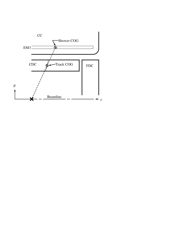
FIG. 1.: The vertex position calculated using the position of the electron cluster (as determined using the information from the third layer of the EM calorimeter) and the center-of-gravity of the electron track (as measured in the tracking chambers).

A total of 5397 events passes the $Z\to ee$ selection criteria, of which 2737 events have both electrons in the CC calorimeter (CC-CC events), 2142 events have one in the CC and one in the EC (CC-EC events), and 518 events have both electrons in the EC calorimeter (EC-EC events). Figure 2 shows the invariant mass distribution of the $Z\to ee$ candidates.

FIG. 2.: The invariant mass distribution from the $Z\to ee$ candidate event sample. The shaded region represents the dielectron invariant mass requirement.

Candidates for the process $W\to e\nu$ are required to have one tight electron with $E_{T}$ $>$ 25 GeV, and ${\hbox{$E$\kern-6.00006pt\lower-0.43057pt\hbox{/}}}_{T}$ $>$ 25 GeV. Events containing a second loose or tight electron with $E_{T}$ $>$ 25 GeV are rejected to reduce backgrounds from $Z/\gamma^{*}\rightarrow ee$ events. The ${\hbox{$E$\kern-6.00006pt\lower-0.43057pt\hbox{/}}}_{T}$ is calculated as the negative of the vector sum of the electron $E_{T}$ and the underlying event and recoil $E_{T}$. The $E_{T}$ from the underlying event and the recoil is calculated as the vector sum of the $E_{T}$ of all calorimeter cells except those which contain the electron. While the electron $E_{T}$ is calculated using the above vertex, the underlying event and recoil $E_{T}$ are calculated using a vertex determined from all tracks in the CDC, called the “standard” vertex, since the electron vertex is not available at the appropriate stage of the event reconstruction. The use of different vertex definitions results in a small degradation of the ${\hbox{$E$\kern-6.00006pt\lower-0.43057pt\hbox{/}}}_{T}$ resolution. For the collected data, the mean number of interactions per crossing is approximately 1.6. For events with more than one interaction vertex, the one with the largest number of associated tracks is selected as the standard vertex (even though it may or may not be the vertex closest to the extrapolated position of the electron track). Figure 3 shows the fraction of events in which the standard vertex is more than 10 cm away from the electron vertex. The figure also shows the $Z\to ee$ invariant mass distribution when the standard vertex is used and when the electron vertex is used. The electron vertex gives a sharper invariant mass distribution, because it has better resolution and little luminosity dependence.

FIG. 3.: (a) Frequency at which the standard vertex, $z_{\rm{standard}}$ (calculated using all tracks), is more than 10 cm away from the extrapolated track position, $z_{e}$, as a function of luminosity. For comparison, the frequency at which $Z\to ee$ events with two tight electrons have extrapolated track positions $z_{1}$ and $z_{2}$ differing by more than 10 cm is shown. (b) Invariant mass distribution for $Z\to ee$ events when the standard vertex position is used and when the electron vertex position is used.

A total of 67078 events passes the $W\to e\nu$ requirements, of which 46792 events have their electron in the CC (CC events), with 20286 events in the EC (EC events). Figure 4 shows the transverse mass distribution of the candidates, where the transverse mass is calculated as

$$M_{T}=\sqrt{2E_{T}(e)\mbox{${\hbox{$E$\kern-6.00006pt\lower-0.43057pt\hbox{/}}}_{T}$}(1-\cos{\delta\phi})}$$ (6)

and $\delta\phi$ is the angle between the electron and the ${\hbox{$E$\kern-6.00006pt\lower-0.43057pt\hbox{/}}}_{T}$ in the transverse plane.

FIG. 4.: The transverse mass distribution from the $W\to e\nu$ candidate event sample.

IV Acceptances and Correction Factors

A Monte Carlo Simulation

The geometric and kinematic acceptances of the selection criteria are calculated using a Monte Carlo simulation. Initially, the $W$ or $Z$ boson, the recoil system, and the underlying event are generated with appropriate kinematic properties and the $W$ or $Z$ boson is forced to decay in the electron channel. A second stage then models the response of the detector and the effect of the geometric and kinematic selection criteria.

The primary event generator, originally developed for the DØ $W$ boson mass analysis, is described in detail in Refs. [18, 19]. The detector simulation was re-tuned for this analysis, because the mass analysis used only electrons with $|\eta_{D}|$ $<$ 1.1 and imposed different fiducial cuts at the azimuthal boundaries of the central calorimeter modules. Also, the mass analysis was restricted to events with $W$ boson $p_{T}$ $<15$ GeV, while this is not the case for the present analysis. The mass distribution of the $W$ or $Z$ boson is generated according to a Breit-Wigner distribution convoluted with the CTEQ4M [20] parton distribution functions, taking account of polarization in the decay. The transverse momentum and rapidity distributions of the $W$ or $Z$ boson are generated by computing the differential cross section, $d^{2}\sigma/dp_{T}^{2}dy$, using a program provided by Ladinsky and Yuan [21], as discussed in Ref. [17]. The $W$ or $Z$ boson decays include the effects of lowest-order internal bremsstrahlung, where a photon is radiated from a final state electron, using the Berends-Kleiss calculation [22]. This calculation predicts that approximately 31% of the $W$ boson events and 66% of the $Z$ boson events have a photon with an energy above 50 MeV in the final state. In the simulation, the energies of the photon and its associated electron are combined if their separation, $\sqrt{\Delta\eta^{2}+\Delta\phi^{2}}$, is less than 0.3, where $\Delta\phi$ is in radians. For the $Z$ boson, events are generated according to the $Z$ boson line shape, and no Drell-Yan or interference terms are included. The generator produces $W$ and $Z$ bosons only over a finite mass range, and we include a small correction in the acceptance to account for this. As a cross check, we have also calculated the acceptances using events generated with the PYTHIA [23] event generator, and the results are consistent with those from our generator.

In the detector modeling phase of the simulation, the primary vertex distribution is generated as a Gaussian with a width of 27 cm and a mean position of $-0.6$ cm, to match the observed distribution. Electron energies and angles are smeared according to measured resolutions and are corrected for offsets in energy scale due to contamination from particles from the underlying event or the recoil in the calorimeter towers containing the electron signal. The electron energy scale is adjusted to reproduce the known mass [16] of the $Z$ boson. The electron energy and angular resolutions used in the Monte Carlo are tuned to reproduce the observed width of the $Z\to ee$ invariant mass distribution for the sample used in this analysis.

The uncertainty in the electromagnetic energy scale is 0.1% for the CC and 1.6% for the EC. The large uncertainty in the EC energy scale is due to a rapidity dependent calibration inaccuracy of the EC calorimeter. We correct for it in each sample which contains EC electrons (CC-EC $Z\to ee$ events, EC-EC $Z\to ee$ events, and EC $W\to e\nu$ events), by fitting the corresponding invariant or transverse mass distributions to the data, and the uncertainty is taken as the size of the correction.

The electron energy resolution ($\Delta E$) can be parametrized as $\Delta E/E={\cal C}\oplus{\cal S}/\sqrt{E_{T}}$, where the two terms are called the constant and sampling term, respectively. The value of $\cal S$ is known to high precision from test beam studies and is $0.135\ \rm{GeV}^{1/2}$ for CC electrons and $0.157\ \rm{GeV}^{1/2}$ for EC electrons. The value of $\cal C$ in the simulation is adjusted until the r.m.s. from the Monte Carlo $Z\to ee$ invariant mass distribution matches that of the data. Figure 5 shows the result of fitting the invariant mass distribution of CC-CC $Z\to ee$ candidates to a Breit-Wigner convoluted with a Gaussian. Figure 6 shows the r.m.s. of the Gaussian that is obtained when the same procedure is applied to Monte Carlo as a function of the CC constant term, along with the result from the data. The intersection of the two gives the constant term. The constant term in the CC is thus determined to be 0.014 $\pm$ 0.002 with the uncertainty being dominated by the statistics of the $Z\to ee$ sample. The constant term in the EC is $0.00^{+0.01}_{-0.00}$.

FIG. 5.: Invariant mass distribution for the CC-CC $Z\to ee$ data sample. A Breit-Wigner convoluted with a Gaussian resolution is fit to this distribution and the width is used to determine the constant term in the CC electron energy resolution. The $\chi^{2}$ per degree of freedom for the fit is 88.7/56.

FIG. 6.: Determination of the constant term for the electron energy resolution. The curved dashed line connecting the Monte Carlo points shows the correlation between the constant term in the CC electron energy resolution and the fitted width of the CC-CC $Z\to ee$ invariant mass distribution from the Monte Carlo. The horizontal solid line shows the fitted width of the CC-CC data sample, and the horizontal dashed lines the uncertainty on the fitted width. From the intersection of the data line with the curved dashed line we determine the constant term for CC electrons to be 0.014 $\pm$ 0.002.

The uncertainty in the polar angle of CC electrons is parametrized as an uncertainty in the position of the track at a radius of 62 cm for CDC tracks. The $z$ position of the track at this radius has a 0.3 cm uncertainty. The uncertainty in the polar angle for EC electrons is absorbed into the large uncertainty in the EC energy scale.

In the simulation, the recoil momentum is smeared by the measured resolution. The recoil is also corrected for any losses of particles to the same calorimeter towers as the electron. The model of the response of the calorimeter to particles recoiling against the $W$ or $Z$ boson is tuned using $Z\to ee$ events. The $\hat{\eta}$ axis is defined as the bisector of the azimuthal angle between the two electrons, as shown in Fig. 7. We compare the component of the $p_{T}$ of the $Z$ boson along $\hat{\eta}$ as calculated using the energies of the electrons, $(p_{T}^{ee})_{\hat{\eta}}$, to that calculated by summing the transverse momentum of all towers in the calorimeter, except those containing the electrons, $(p_{T}^{\rm{rec}})_{\hat{\eta}}$.

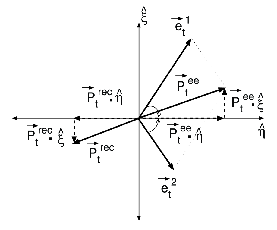
FIG. 7.: Definition of the $\hat{\eta}$–$\hat{\xi}$ coordinate system in a $Z\to ee$ event. The $\hat{\eta}$ axis is the bisector of the electron directions in the transverse plane; the $\hat{\xi}$ axis is perpendicular to $\hat{\eta}$.

Because the calorimeter response is different for electrons and for recoil particles, the algebraic sum of $(p_{T}^{\rm{rec}})_{\hat{\eta}}$ and $(p_{T}^{\rm{ee}})_{\hat{\eta}}$ is on average non zero. The average value of this “$\hat{\eta}$-imbalance” scales linearly with $(p_{T}^{ee})_{\hat{\eta}}$, as shown in Fig. 8. The recoil scale used in the simulation is tuned such that applying the same procedure to Monte Carlo events yields the same response as the data. Figure 9 shows the slope of the average $(p_{T}^{\rm{rec}})_{\hat{\eta}}+(p_{T}^{\rm{ee}})_{\hat{\eta}}$ versus $(p_{T}^{ee})_{\hat{\eta}}$ from the Monte Carlo as a function of the hadronic scale, along with the slope determined from data. The intersection of the two determines the hadronic response to be $\alpha_{H}=0.753\pm 0.024$ relative to the electromagnetic energy scale, with the uncertainty being dominated by uncertainties in the EC electromagnetic energy scale. The hadronic energy resolution is parametrized in the same way as the electron energy resolution, and is known from jet studies to have a constant term of 4% and a sampling term of $0.8/\sqrt{p_{T}/\rm{GeV}}$.

FIG. 8.: The $\hat{\eta}$-imbalance, $(p_{T}^{\rm{rec}})_{\hat{\eta}}+(p_{T}^{\rm{ee}})_{\hat{\eta}}$, versus $(p_{T}^{ee})_{\hat{\eta}}$ from the $Z\to ee$ sample. The solid line is a linear fit to the data points, with a slope of 0.239 $\pm$ 0.006 and a $\chi^{2}$ per degree of freedom of 47.5/23. Up to a $p_{T}$ of 25 GeV, where most of the $W\to e\nu$ and $Z\to ee$ data is, the $\chi^{2}$ per degree of freedom is 1.2. The hadronic response contributes only a small fraction of the uncertainty in the acceptance.

FIG. 9.: Determination of the hadronic scale $\alpha_{H}$. The points represent the slope of the line $(p_{T}^{\rm{rec}})_{\hat{\eta}}+(p_{T}^{\rm{ee}})_{\hat{\eta}}$ versus $(p_{T}^{ee})_{\hat{\eta}}$ obtained from Monte Carlo as a function of $\alpha_{H}$. The intersection of the dashed line connecting the Monte Carlo points with the solid line, obtained from data, determines the hadronic scale used in the simulation. We take $\alpha_{H}=0.753\pm 0.024$.

The underlying event is modeled using events taken with a LØ trigger (minimum bias events) with the same luminosity profile as the $W$ and $Z$ boson samples. We pick a minimum bias event randomly from this sample and its ${\hbox{$E$\kern-6.00006pt\lower-0.43057pt\hbox{/}}}_{T}$ is combined vectorially with that of the simulated $W$ boson. To account for any possible difference between the underlying event in $W$ boson and in minimum bias events, we introduce a multiplicative scale factor for the $E_{T}$ of the minimum bias events. The scale factor is estimated using the $Z\to ee$ sample and set so that the width of the “$\hat{\eta}$-balance” distribution from the simulation agrees with that from the data, where “$\hat{\eta}$-balance” is $(p_{T}^{\rm{rec}}/\alpha_{H}+p_{T}^{ee})_{\hat{\eta}}$. Figure 10 shows this quantity for the $Z\to ee$ event sample. Figure 11 shows the r.m.s. of the $(p_{T}^{\rm{rec}})_{\hat{\eta}}$ distribution from the simulation as a function of the minimum bias scale factor. The simulation has the same r.m.s. as the data when the scale factor between the minimum bias events and the $W$ boson underlying events is 1.01 $\pm$ 0.02.

FIG. 10.: Distribution of the “$\hat{\eta}$-balance,” the magnitude of the vectorial sum of $(p_{T}^{\rm{rec}})_{\hat{\eta}}/\alpha_{H}$ and $(p_{T}^{ee})_{\hat{\eta}}$, for events in the $Z\to ee$ sample (solid histogram), and for Monte Carlo (dashed histogram).

FIG. 11.: Determination of the minimum bias scale factor. The points represent the r.m.s. of the $\hat{\eta}$-balance distribution from Monte Carlo as a function of the minimum bias scale factor. The solid horizontal line shows the r.m.s. from the data sample. The intersection of the dashed line connecting the Monte Carlo points with the data line determines the minimum bias scale factor used in the simulation to be $1.01\pm 0.02$.

Figure 12 shows the electron detector pseudorapidity distribution, $\eta_{D}$, for $Z\to ee$ candidates and for the Monte Carlo after all cuts and corrections have been applied. The sharp edges correspond to the fiducial requirements applied to the electrons. The data and the Monte Carlo agree well. Since the tracking efficiency is obtained from the $Z$ data (as explained in Sec. V), the figure shows electrons without the tracking requirement.

FIG. 12.: The electron $\eta_{D}$ distribution for $Z\to ee$ candidates (solid circles) and for the Monte Carlo (histogram) after all corrections and cuts except for track match have been applied. The error bars represent the statistical uncertainty in the data. The $\chi^{2}$ per degree of freedom is 0.65.

B Geometric and Kinematic Acceptance

The acceptance is defined as the fraction of generated $W\to e\nu$ or $Z\to ee$ events satisfying the kinematic and geometric requirements. Samples of 25,000,000 events are used to estimate all systematic uncertainties, except those from ambiguities in the parton distribution functions and differences in generators. For these, we use the slower PYTHIA generator and samples of 1,000,000 events, corresponding to statistical errors of 0.1%, which are small compared to the dominant uncertainties. Table I shows the acceptance results and a summary of the systematic uncertainties.

TABLE I.: Acceptances and their systematic uncertainties for $W$ and $Z$ boson events and their ratio.

	$A_{W}$	$A_{Z}$	$\frac{A_{W}}{A_{Z}}$
Acceptance	0.465 $\pm$ 0.004	0.366 $\pm$ 0.003	0.787 $\pm$ 0.007
Error source	$\frac{\delta A_{W}}{A_{W}}$ [%]	$\frac{\delta A_{Z}}{A_{Z}}$ [%]	$\delta\left(\frac{A_{Z}}{A_{W}}\right)/\left(\frac{A_{Z}}{A_{W}}\right)$ [%]
$p_{T}$ spectrum	0.096	0.104	0.100
Parton distribution functions	0.189	0.314	0.252
Clustering algorithm	0.141	0.294	0.153
$\delta M_{W}$	0.130	—	0.130
$\delta\Gamma_{W}$	0.050	—	0.050
EM energy scale	0.685	0.337	0.698
EM energy resolution	0.024	0.037	0.044
Hadronic response	0.129	—	0.129
Hadronic resolution	0.078	—	0.078
Angular resolution	0.019	0.046	0.027
Generated mass range	0.150	0.180	0.234
Generator	0.343	0.516	0.172
Total	0.85%	0.78%	0.85%

The uncertainties in the $W$ and $Z$ boson $p_{T}$ spectra are calculated by varying the theoretical parameters in Ref. [21] within the range quoted by the authors. The systematic uncertainties from the choice of parton distribution functions are calculated from the largest excursion in acceptance found using the CTEQ4M [20], CTEQ2M [20], MRSD$-$ [25], MRS(G) [26], GRV94HO [27], and versions of the MRSA^′ distribution functions with values of the strong coupling constant ranging from 0.150 to 0.344 [28].

The systematic uncertainties in the acceptance due to the presence of radiative photons in the event come from uncertainties on the minimum separation in $\eta$-$\phi$ space the electron and the photon must have in order to be resolved as separate clusters by our calorimeter clustering algorithm. The uncertainties due to effects of the clustering algorithm are calculated by varying the size of the cone that is used to decide whether or not the photon will be resolved from the electron in the detector between 0.2 and 0.4.

We use a $W$ boson mass of 80.375 GeV  and width of 2.066 GeV, and vary these by $\pm 0.065$ GeV and $\pm 0.060$ GeV, respectively. The $W$ boson mass is the result of combining the measurements from DØ [17], CDF [24], and a fit to all direct $W$ boson mass measurements from LEP [16]. The $W$ boson width is the current world average [2, 3, 4, 5, 6, 7]. The systematic uncertainties in the acceptance due to the EM energy scale, EM resolution, hadronic response, hadronic resolution, and the resolution on the polar angle of electron tracks are found by varying the relevant parameters within the Monte Carlo simulation by their individual uncertainties.

The generation of $W$ and $Z$ bosons is limited to the mass ranges 40–120 GeV for $W$ bosons and 30–150 GeV for $Z$ bosons. The error quoted on generated mass in Table I is the uncertainty on the fraction of events outside this mass window that would pass our selection criteria. The error is dominated by the statistics of the Monte Carlo samples, but is well below the dominant uncertainties. The error quoted on the generator is from a comparison of the difference in acceptance between our Monte Carlo and PYTHIA (after smearing PYTHIA for detector response).

The acceptances and their uncertainties for $W\to e\nu$, $Z\to ee$, and their ratio are shown in Table I. The $W$ boson acceptance is $A_{W}=0.465\pm 0.004$. The largest contributions to the uncertainty arise from uncertainties in the EM energy scale, the width of the $W$ boson, the difference between our generator and PYTHIA, and uncertainties in the parton distribution functions. The acceptance for $Z\to ee$ events is $A_{Z}=0.366\pm 0.003$. The largest sources of systematic uncertainty arise from the difference between our generator and PYTHIA, effects of the electron-photon clustering algorithm in radiative $Z$ boson decays, and uncertainties in the EM energy scale and in the parton distribution functions. In the ratio of acceptances, a few of the systematic uncertainties are reduced by partial cancelations of correlated errors. The ratio of the acceptances is $A_{Z}/A_{W}=0.787\pm 0.007$.

C Drell-Yan Correction

It is conventional to report $\sigma(p\overline{p}\rightarrow Z+X)\cdot B(Z\rightarrow ee)$ as the product of the cross section and branching ratio, assuming the $Z$ boson as the only source of dielectron events. However, the production of dielectron events is properly described by considering the $Z$ boson, the photon propagator, and the interference between the two. The Drell-Yan correction factor relates the number of events in our mass window to what would be expected purely from $Z$ boson production. To obtain this correction, we use PYTHIA to generate events with just the contribution from the $Z$ boson, and, separately, using the full Drell-Yan process with interference terms (combining $Z$ boson and photon diagrams). We process both samples with the same Monte Carlo simulation used for the acceptance calculation. The ratio of the complete Drell-Yan cross section ($\sigma_{DY}$) to the cross section for the $Z$ boson alone ($\sigma_{Z}$), for events passing our $Z\to ee$ selection criteria, is estimated to be

$$\sigma_{DY}/\sigma_{Z}=\frac{1}{1-f_{DY}}=1.012\pm 0.001$$ (7)

or $f_{DY}$ = 0.012 $\pm$ 0.001 as the fraction of production cross section attributable to the presence of the photon propagator. The systematic uncertainty is evaluated by using the ISAJET [29] generator instead of PYTHIA and is estimated as the difference between the two generators. The primary uncertainty in $f_{DY}$ is due to Monte Carlo statistics, but its contribution to the total uncertainty in the $Z$ boson cross section and in $R$ is negligible.

D NLO Electroweak Radiative Corrections

Next to leading order (NLO) electroweak processes modify the cross sections and their ratio [30]. A full NLO calculation is available for the $W$ boson which suggests that the $W$ boson cross section would decrease by a multiplicative factor of $0.998\pm 0.001$ [31]. For the $Z$ boson, only the full QED calculation is available; the purely weak part is missing. For the ratio $\cal R$, the best theoretical estimate at this time is a multiplicative factor of $1.00\pm 0.01$ [31], where the uncertainty is dominated by the difference between the NLO corrections to the $W$ and $Z$ boson cross sections, due mainly to the purely weak corrections missing in the $Z$ boson calculation. This theoretical uncertainty is expected to be reduced in the future. A 1% uncertainty in $\cal R$ due to NLO electroweak radiative corrections is quoted in this analysis.

V Efficiencies

A Electron Identification Efficiencies

Electron identification efficiencies are obtained using $Z\to ee$ events selected by requiring two electron candidates satisfying only standard kinematic and fiducial requirements. An electron is considered a “probe” electron if the other electron in the event passes all standard electron identification criteria. This gives a clean and unbiased sample of electrons. We count the number of events inside a $Z$ boson invariant mass $m(ee)$ window before and after applying the electron identification criteria to each probe electron. The ratio of the number of events in the $Z$ boson mass window, after background subtraction, gives the electron identification efficiency. Two techniques are used to determine the background. In the sideband method, the number of $Z\to ee$ events in the regions 60 $<$ $m(ee)$ $<$ 70 GeV and 110 $<$ $m(ee)$ $<$ 120 GeV is used to estimate the number of events inside the signal region by assuming a linear shape for the background. In the second method, backgrounds are estimated by fitting the observed invariant mass distribution to a Breit-Wigner (smeared with a Gaussian to account for detector resolution) for the $Z$ boson, and an assumed first-order polynomial for the background. The background is estimated from the contribution of the polynomial within the signal region. The difference between these two estimates comprises a part of the systematic uncertainty, which also includes the sensitivity of the result to the band chosen as the signal region. We have also used an exponential shape for the background, and the efficiencies resulting from such a fit are all well within the corresponding uncertainties. We have checked for any dependence of the efficiency on the $E_{T}$ of the electron, and find none.

The above method does not yield the correct efficiency when the probability for one of the electrons to pass the identification requirements is correlated with that of the other. We check for such correlations in the calorimeter-based identification requirements using a GEANT-based simulation [32]. We find that the impact of such a correlated bias is small compared to the uncertainty on the efficiency, and we neglect it. For tracking-based electron identification requirements, we evaluate the correlations using data and find that these correlations can not be neglected. We select events with two electrons that pass the geometric and calorimetric electron identification requirements of the $Z\to ee$ data sample. We count the background-subtracted number of $Z\to ee$ events that have both electrons passing the tracking requirements ($N_{PP}$), only one electron passing the tracking requirements ($N_{PF}$), and with no electrons passing the requirements ($N_{FF}$). The efficiency for a $W$ boson to pass the tracking requirements is then $\left(2N_{PP}+N_{PF}\right)/\left[2\left(N_{PP}+N_{PF}+N_{FF}\right)\right]$. The efficiency for a $Z$ boson to pass the tracking requirements is $\left(N_{PP}+N_{PF}\right)/\left(N_{PP}+N_{PF}+N_{FF}\right)$. The tracking efficiency for a $W$ boson or a $Z$ boson is found to be 1.7 $\pm$ 0.3% lower than what one would get assuming no correlations. The effect of this correlation cancels in the ratio of the cross sections [33].

The efficiency of the calorimetric requirements is 0.916 $\pm$ 0.006 for CC electrons and 0.870 $\pm$ 0.007 for EC electrons. The efficiency of the tracking requirements is 0.777 $\pm$ 0.006 for CC electrons in $W$ boson events and 0.731 $\pm$ 0.010 for EC electrons in $W$ boson events. (Because of the presence of correlations, the per track efficiency is not a useful concept for $Z$ boson events.)

B Trigger Efficiencies

Trigger efficiencies are evaluated from different data samples. A special trigger which is identical to the $W\to e\nu$ trigger, except for its ${\hbox{$E$\kern-6.00006pt\lower-0.43057pt\hbox{/}}}_{T}$ requirement, is used to evaluate the relative efficiency of the ${\hbox{$E$\kern-6.00006pt\lower-0.43057pt\hbox{/}}}_{T}$ requirement in the $W$ boson trigger. The efficiency of the ${\hbox{$E$\kern-6.00006pt\lower-0.43057pt\hbox{/}}}_{T}$ requirement is found to be 0.993 $\pm$ 0.001. The efficiency of the electron requirements in the trigger is measured from a dielectron sample using the same method used to determine the electron identification efficiencies, and is found to be $0.995\pm 0.001$ for electrons in the CC, and $0.996\pm 0.002$ for electrons in the EC. A portion of the $W\to e\nu$ data was taken without requiring the LØ component of the trigger. By studying these events, and taking into account the luminosity-dependent effects, we find the LØ efficiency for $W$ boson events to be $0.986\pm 0.005$. We assume that this efficiency is the same for $W\to e\nu$ and for $Z\to ee$ events, and therefore cancels in the ratio.

C Total Efficiencies

The efficiency for a $W$ or $Z$ boson to pass the electron identification requirements is obtained from the convolution of the efficiencies with the acceptances as a function of the $\eta$ of the electrons from our Monte Carlo. From our Monte Carlo simulation, of the events that pass our kinematic and geometric selection, 68.70% of $W$ bosons have a CC electron and 31.30% have an EC electron. For the $Z$ boson, 49.69% have both electrons in the CC, 40.55% have one CC and one EC  electron, and 9.76% have both electrons in the EC. The efficiency for $W$ bosons to pass both the electron identification and the trigger requirements is 0.685 $\pm$ 0.008. The analogous efficiency for $Z$ bosons is 0.754 $\pm$ 0.011.

Taking into account the LØ efficiency, the total efficiency for $Z$ bosons is $\epsilon_{Z}=0.744\pm 0.011$. For the $W$ boson, combining electron identification and trigger efficiencies with the efficiencies of the ${\hbox{$E$\kern-6.00006pt\lower-0.43057pt\hbox{/}}}_{T}$ and LØ requirements, we obtain a total efficiency of $\epsilon_{W}=0.671\pm 0.009$. The ratio of the efficiencies is $1.108\pm 0.007$, where the error takes into account the correlations between the uncertainties in the $W$ and $Z$ boson efficiencies.

D Diffractive Production of Weak Bosons

Diffractive production of $W$ and $Z$ bosons at the Tevatron occurs when the incident proton or anti-proton escapes intact, losing a small fraction of its initial forward momentum. Our cross section measurements include both diffractive and non-diffractive $W$ and $Z$ boson production. The perturbative theoretical calculation of Ref. [9] does not include an explicit calculation of diffraction, but diffraction contributions to the total cross sections enter through the parton distribution functions. A recent measurement [34] reports the diffractive to non-diffractive $W$ boson production ratio to be $(1.15\pm 0.55)\%$. No such measurement exists to date for $Z$ bosons, although it is believed that diffractive $Z$ boson production exists at roughly the same level. Recent theoretical calculations suggest that the ratio of diffractive $W$ to $Z$ boson cross sections is roughly the same as the ratio of inclusive cross sections (see Table V of Ref. [35]). Since the LØ trigger requires simultaneous hits in the forward and backward scintillation counters, such events would not pass our selection unless accompanied by a minimum bias interaction. The LØ trigger efficiency is calculated from $W$ boson events without a LØ requirement, and no correction is made to subtract diffractive $W$ bosons, so in practice we account for all diffractive $W$ bosons produced. The same efficiency is used for $Z$ boson events under the assumption that the underlying events in $W$ and $Z$ boson production are essentially identical. In order to have an appreciable effect on $R$, the diffractive production of $Z$ bosons would have to be several times larger than that observed for $W$ bosons, so we may safely neglect the effect on $R$. The effects of diffractive production on the individual cross sections are much smaller than the luminosity uncertainty and are therefore neglected.

VI Backgrounds

A Backgrounds from multijet, $b$ quark, and direct photon sources in the $W\to e\nu$  sample

The fraction of background events in the $W\to e\nu$ sample that is due to multijet, $b$ quark, and direct photon sources, $f_{QCD}$ (also referred to as QCD background), is calculated by comparing the number of events in the $W\to e\nu$ sample to the number in a sample with the same kinematic requirements, but with loosened or tightened electron-identification requirements. The larger sample is the “parent” sample, the smaller the “child.” If the efficiency for signal and for background to pass the child criteria relative to the parent requirements is known, the number of signal and background events can be simply calculated. The efficiency for electrons from $W$ boson decay to pass the identification requirements $(\epsilon_{s})$ is calculated using the $Z\to ee$ sample. The efficiency for “electrons” from background sources $(\epsilon_{b})$ is calculated using a data sample obtained using the same criteria as the $W\to e\nu$ sample, except requiring small ${\hbox{$E$\kern-6.00006pt\lower-0.43057pt\hbox{/}}}_{T}$ in the event instead of large ${\hbox{$E$\kern-6.00006pt\lower-0.43057pt\hbox{/}}}_{T}$ (to remove $W$ boson events). The main source of systematic uncertainty is from the assumption that the “electrons” from background sources in events with small ${\hbox{$E$\kern-6.00006pt\lower-0.43057pt\hbox{/}}}_{T}$ have the same value for $\epsilon_{b}$ as those with ${\hbox{$E$\kern-6.00006pt\lower-0.43057pt\hbox{/}}}_{T}$ $>$ 25 GeV. We evaluate this uncertainty by varying the ${\hbox{$E$\kern-6.00006pt\lower-0.43057pt\hbox{/}}}_{T}$ cutoff used to define the background sample (we use the ${\hbox{$E$\kern-6.00006pt\lower-0.43057pt\hbox{/}}}_{T}$ ranges 0–5, 0–10, 0–15, and 10–15 GeV), and by using different parent and child requirements.

We define our parent and child samples by varying the shower shape requirements and by tightening the selection by requiring the $dE/dx$ measured in the tracking system to be consistent with that of an electron. Tables II and III show the results.

TABLE II.: The fraction of the $W\to e\nu$ events in the CC that come from multijet, $b$ quark, and direct photon sources, $f_{QCD}^{W\ {\rm CC}}$. In this table, ISO refers to the electron isolation requirement, EMF to the requirement that the fraction of the electron energy in the hadronic calorimeter be small, CHI refers to the shower shape requirement, nominal means the electron identification criteria used in the $W\to e\nu$ sample (CHI$<$100, ISO$<$0.15, and EMF$>$ 0.95, see Ch.3 of Ref. [12]). $dE/dx$ means the matching track was required to have $dE/dx<1.4$ or $dE/dx>3.0$ for CDC tracks and $dE/dx<1.3$ or $dE/dx>2.5$ for FDC tracks, to reject photon conversions (see Ref. [36]).

Parent cuts	Child Cuts	$\epsilon_{s}$	$\epsilon_{b}$	$f_{QCD}^{W\ {\rm CC}}$ [%]
nominal	+$dE/dx$	0.933 $\pm$ 0.004	0.372 $\pm$ 0.023	3.39$\pm$0.9
ISO(0.15),EMF(0.95)	nominal	0.952 $\pm$ 0.003	0.686 $\pm$ 0.017	4.49$\pm$1.0
EMF(0.95)	nominal	0.949 $\pm$ 0.003	0.650 $\pm$ 0.011	4.41$\pm$0.8
EMF(0.9)	nominal	0.941 $\pm$ 0.004	0.573 $\pm$ 0.015	4.46$\pm$0.8
EMF(0.9),ISO(0.15)	nominal	0.945 $\pm$ 0.004	0.621 $\pm$ 0.016	4.76$\pm$0.8
EMF(0.9),CHI(100)	nominal	0.989 $\pm$ 0.003	0.872 $\pm$ 0.007	6.16$\pm$2.0
ISO(0.15),CHI(100)	nominal	0.992 $\pm$ 0.002	0.934 $\pm$ 0.007	6.96$\pm$3.0

TABLE III.: The fraction of the $W\to e\nu$ events in the EC that come from multijet, $b$ quark, and direct photon sources, $f_{QCD}^{W\ {\rm EC}}$. In this table, ISO refers to the electron isolation requirement, EMF to the requirement that the fraction of the electron energy in the hadronic calorimeter be small, CHI refers to the shower shape requirement, nominal means the electron identification criteria used in the $W\to e\nu$ sample (CHI$<$100, ISO$<$0.15, and EMF $>$ 0.95, see Ch. 3 of Ref. [12]). $dE/dx$ means the matching track was required to have $dE/dx<1.4$ or $dE/dx>3.0$ for CDC tracks and $dE/dx<1.3$ or $dE/dx>2.5$ for FDC tracks (see Ref. [36]).

Parent cuts	Child Cuts	$\epsilon_{s}$	$\epsilon_{b}$	$f_{QCD}^{W\ {\rm EC}}$ [%]
nominal	+$dE/dx$	0.759 $\pm$ 0.010	0.552 $\pm$ 0.007	14.60$\pm$4.5
ISO(0.15),EMF(0.95)	nominal	0.881 $\pm$ 0.009	0.513 $\pm$ 0.016	11.03$\pm$1.5
EMF(0.95)	nominal	0.880 $\pm$ 0.009	0.492 $\pm$ 0.015	11.44$\pm$1.2
EMF(0.9)	nominal	0.868 $\pm$ 0.010	0.367 $\pm$ 0.015	14.48$\pm$1.2
EMF(0.9),ISO(0.15)	nominal	0.868 $\pm$ 0.009	0.398 $\pm$ 0.017	14.13$\pm$1.4
EMF(0.9),CHI(100)	nominal	0.987 $\pm$ 0.004	0.858 $\pm$ 0.013	19.99$\pm$3.3
ISO(0.15),CHI(100)	nominal	0.991 $\pm$ 0.003	0.897 $\pm$ 0.010	21.94$\pm$3.8

The uncertainty on the background fraction is dominated by the uncertainties on $\epsilon_{s}$ and $\epsilon_{b}$, and is given approximately by

$$\delta f^{W}_{QCD}\approx\frac{\epsilon_{s}}{\epsilon_{s}-\epsilon_{b}}\delta\epsilon_{s}\oplus\frac{\epsilon_{b}f^{W}_{QCD}}{\epsilon_{s}-\epsilon_{b}}\delta\epsilon_{b}.$$ (8)

From this equation, one can see that the method works best when $\epsilon_{s}-\epsilon_{b}$ is large, and produces large errors when this difference is small. We take a Gaussian distribution (normalized to unity) with the mean and uncertainty corresponding to each background fraction in Tables II and III. For the mean value of $f^{W}_{QCD}$, we add all the CC or EC distributions and take the median of the resulting distribution. We set the systematic uncertainty in $f^{W}_{QCD}$ from the symmetric band around the median with an area of 68% of the total distribution. The results are $f^{W\ {\rm CC}}_{QCD}=0.046\pm 0.014$ for CC events, and $f^{W\ {\rm EC}}_{QCD}=0.143\pm 0.043$ for EC events. To obtain the combined background fraction, we combine the CC and EC $W$ boson cross sections. The weights for CC and EC events are taken as $1/\delta_{u}^{2}$ , where $\delta_{u}$ is the total uncorrelated error for each individual cross section, and where we make the conservative assumption that there is maximal correlation between the CC and EC uncertainties (the correlated part for each uncertainty is the smaller of the two). We then find the background fraction that corresponds to this combined $W$ boson cross section. The combined background fraction is estimated to be $f^{W}_{QCD}=0.064\pm 0.014$.

The method we use to obtain $\epsilon_{b}$ assumes that the efficiency for background events to pass the electron identification requirements is the same for events with small and large ${\hbox{$E$\kern-6.00006pt\lower-0.43057pt\hbox{/}}}_{T}$. Most of our identification requirements are calorimeter-based and can, in principle, be correlated with ${\hbox{$E$\kern-6.00006pt\lower-0.43057pt\hbox{/}}}_{T}$. However, the $f^{W}_{QCD}$ measurement obtained by adding the tracking-based $dE/dx$ requirement yields results consistent with the calorimeter-based methods, giving us confidence that the correlations between ${\hbox{$E$\kern-6.00006pt\lower-0.43057pt\hbox{/}}}_{T}$ and $\epsilon_{b}$ are small. Our studies assume the contamination from the $W$ boson in the backgrounds is small in the low ${\hbox{$E$\kern-6.00006pt\lower-0.43057pt\hbox{/}}}_{T}$ region. We check the validity of this assumption by looking at the ${\hbox{$E$\kern-6.00006pt\lower-0.43057pt\hbox{/}}}_{T}$ distributions of the child and parent samples and compare them to the ${\hbox{$E$\kern-6.00006pt\lower-0.43057pt\hbox{/}}}_{T}$ distribution from $W\to e\nu$ and $W\to\tau\nu\to e\nu\overline{\nu}\nu$ Monte Carlo events. Figure 13 shows the case where the parent background sample corresponds to the nominal $W$ boson selection (except for the ${\hbox{$E$\kern-6.00006pt\lower-0.43057pt\hbox{/}}}_{T}$ requirement) and the child sample is obtained from the additional $dE/dx$ requirement. The Monte Carlo distribution is normalized to the background sample distributions in the high ${\hbox{$E$\kern-6.00006pt\lower-0.43057pt\hbox{/}}}_{T}$ region, which is dominated by real $W$ boson events. The fraction of $W$ boson events in the low ${\hbox{$E$\kern-6.00006pt\lower-0.43057pt\hbox{/}}}_{T}$ region is found to be negligible.

FIG. 13.: The ${\hbox{$E$\kern-6.00006pt\lower-0.43057pt\hbox{/}}}_{T}$ distribution for a particular choice of parent and child inclusive electron samples. The solid line is the parent sample corresponding to the nominal $W$ boson selection cuts except for ${\hbox{$E$\kern-6.00006pt\lower-0.43057pt\hbox{/}}}_{T}$. The dashed line is the child sample, corresponding to nominal cuts and the additional $dE/dx$ requirement. The dot-dash line is the sum of $W\to e\nu$ and $W\to\tau\nu\to e\nu\overline{\nu}\nu$ from Monte Carlo. There is negligible $W$ boson contribution in the low ${\hbox{$E$\kern-6.00006pt\lower-0.43057pt\hbox{/}}}_{T}$ background regions.

B Backgrounds from multijet, $b$ quark, and direct photon sources in the $Z\to ee$  sample

The background fraction for the $Z\to ee$ sample due to multijet, $b$ quark, and direct photon sources is determined by fitting the dielectron invariant mass distribution to a linear combination of a signal shape, obtained from $Z/\gamma^{*}$ events generated with PYTHIA and processed through the detector simulation, and a background shape determined from data. Different mass distributions from different sources, such as multijet events, direct photon candidates, and events passing all of the $Z\to ee$ kinematic cutoffs, but failing the electron identification requirements, are used for background shapes. Figures 14, 15, and 16 show such fits with a background shape determined from direct photon data, for the case where both electrons are in the CC, for the case where one electron is in the CC and the other in the EC, and for the case where both electrons are in the EC, respectively. Systematic uncertainties are determined from the range of values obtained using the different background shapes and by varying the range of invariant masses used in the fit. The result is $f^{Z}_{QCD}=0.045\pm 0.005$.

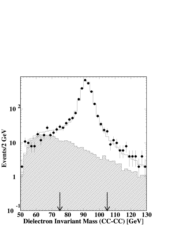
FIG. 14.: Fit of the $Z\to ee$ invariant mass distribution. The shaded histogram is the background shape obtained from direct photon data, and the dots are the $Z\to ee$ candidates. The solid line histogram results from fitting the data to a linear combination of the Drell-Yan signal shape from PYTHIA and the background shape.

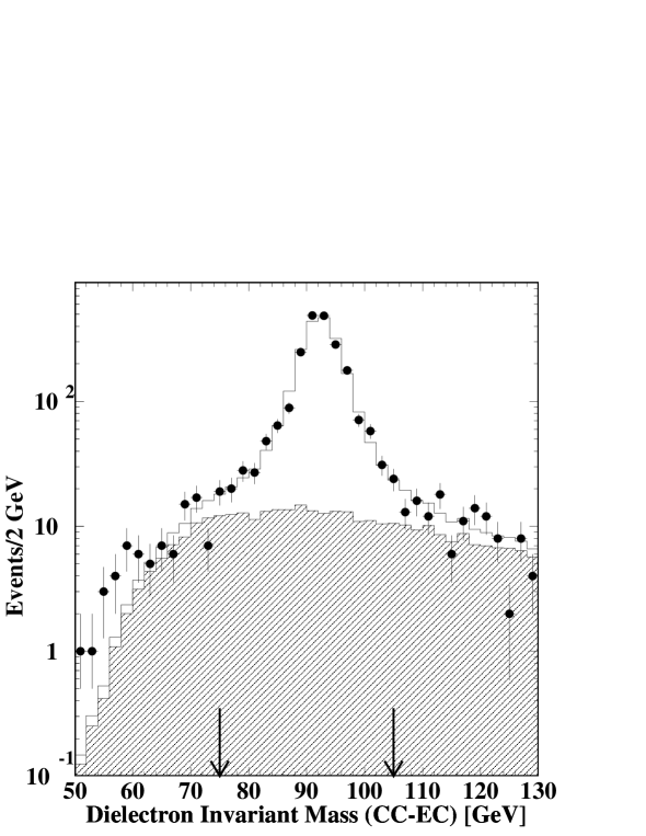
FIG. 15.: Fit of the $Z\to ee$ invariant mass distribution. The shaded histogram is the background shape obtained from direct photon data, and the dots are the $Z\to ee$ candidates. The solid line histogram results from fitting the data to a linear combination of the Drell-Yan signal shape from PYTHIA and the background shape.

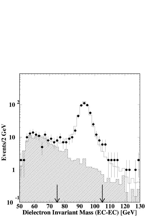
FIG. 16.: Fit of the $Z\to ee$ invariant mass distribution. The shaded histogram is the background shape obtained from direct photon data, and the dots are the $Z\to ee$ candidates. The solid line histogram results from fitting the data to a linear combination of the Drell-Yan signal shape from PYTHIA and the background shape.

C $W$ and $Z$ Boson Backgrounds in the $W\to e\nu$ Sample

The other sources of background in the $W\to e\nu$ sample are $Z\to ee$, $Z\to\tau\tau$, and $W\to\tau\nu$ events. A $Z\to ee$ event can be misidentified as a $W\to e\nu$ event when one of the electrons fails the fiducial requirements or is misidentified as a jet, and the transverse energy in the event is substantially mismeasured, yielding a large apparent ${\hbox{$E$\kern-6.00006pt\lower-0.43057pt\hbox{/}}}_{T}$. Events from the process $Z\to\tau\tau$ can also mimic $W\to e\nu$ events. $W\to\tau\nu$ events, in which the $\tau$ decays to an electron, are identical to $W\to e\nu$ events, except that on average the electron $E_{T}$ and the ${\hbox{$E$\kern-6.00006pt\lower-0.43057pt\hbox{/}}}_{T}$ are lower. The size of these backgrounds scales with the $W\to e\nu$ or $Z\to ee$ cross section, and this must be taken into account when the background subtraction is done. To take this into account, we determine $\sigma(p\overline{p}\rightarrow W+X)\cdot B(W\rightarrow e\nu)$ from the relationship

$$N_{W} = N^{W}_{obs}(1-f^{W}_{QCD})=N_{e}+N_{\tau}+N_{Z}^{W}$$ (9)

$$= \left[\epsilon_{W}\cdot A_{W}\cdot{\sigma(p\overline{p}\rightarrow W+X)\cdot B(W\rightarrow e\nu)}\cdot{\cal L}\right]+$$ (11)

$$\left[\epsilon_{W}\cdot A_{W\tau}^{W}\cdot{\sigma(p\overline{p}\rightarrow W+X)\cdot B(W\rightarrow\tau\nu)}\cdot{\cal L}\right]+N_{Z}^{W}$$

where $N_{W}$ is the number of candidate $W$ boson events after correcting for backgrounds from multijets, direct photons, and $b$ quarks; $N^{W}_{obs}$ is the number of candidate $W\to e\nu$ events; $N_{e}$ is the number of $W\to e\nu$ events passing the $W\to e\nu$ selection criteria; $N_{\tau}$ and $N_{Z}^{W}$ are the numbers of $W\to\tau\nu$ and $Z\to ee$ events respectively passing these criteria; $A_{W\tau}^{W}$ is the fraction of the $W\to\tau\nu$ events that passes the $W\to e\nu$ selection criteria; and $\cal L$ is the integrated luminosity. We assume in Eq. 11 that the $W$ boson couples with equal strength to all lepton flavors, and therefore $B(W\rightarrow\tau\nu)=B(W\rightarrow e\nu)$.

The $Z\to ee$ and $Z\to\tau\tau$ backgrounds are estimated using a GEANT-based simulation of the detector, with HERWIG [37] to generate both $Z\to ee$ and $Z\to\tau\tau$ events. The number of $Z$ boson background events in the $W\to e\nu$ sample is estimated by

$$N^{W}_{Z}=\epsilon_{W}\cdot N_{obs}^{Z}(1-f_{QCD}^{Z})\cdot\frac{A_{Zee}^{W}+A_{Z\tau}^{W}}{A_{Z}\cdot\epsilon_{Z}}$$ (12)

where $A^{W}_{Zee}$ is the fraction of $Z\to ee$ events that passes the $W\to e\nu$ selection criteria; $A^{W}_{Z\tau}$ is the fraction of $Z\to\tau\tau$ events that passes the $W\to e\nu$ selection criteria; $N_{obs}^{Z}$ is the number of candidate $Z\to ee$ events; $f_{QCD}^{Z}$ is the fraction of these candidates from multijet, $b$ quark, and direct photon background sources; $\epsilon_{Z}$ is the electron identification efficiency for $Z\to ee$ events; and $A_{Z}$ is the geometric and kinematic acceptance for $Z\to ee$ events. The ratio $(A_{Zee}^{W}+A_{Z\tau}^{W})/A_{Z}$ is found to be $0.133\pm 0.034$, and thus a total of $621\pm 155$ $Z$ boson events is expected to pass the $W\to e\nu$ selection. The uncertainty in this estimate has two main components: the difference between the electron identification efficiency in the simulation and in the data, and the effect of any additional overlapping minimum-bias events. This uncertainty has a negligible effect on the overall uncertainty in the $W$ boson cross section and the ratio $\cal R$.

The backgrounds to the $W\to e\nu$ and $Z\to ee$ samples from the decays $W\to\tau\nu$ and $Z\to\tau\tau$, where $\tau\rightarrow e\nu$, are calculated using the same $W$ and $Z$ boson production and decay model as in the acceptance calculation. The tau leptons are forced to decay electronically and then the event is smeared. Backgrounds from $\tau$ in the $Z\to ee$ sample are found to be negligible. Assuming lepton universality and the fact that we do not observe any dependence of the lepton identification efficiency on the transverse energy of the lepton, we can account for the $\tau$ backgrounds in the $W$ boson sample by making a correction to the $W$ boson acceptance of $(1+\frac{A_{W\tau}^{W}}{A_{W}})=1.021\pm 0.002$.

VII Luminosity

A precise value of the integrated luminosity is needed for determining any absolute cross section. This analysis uses data collected at $\sqrt{s}$ = 1.8 TeV during the 1994–1995 running of the Fermilab Tevatron. The measurement of luminosity is described in detail in Refs. [12, 13]. The luminosity ($L$) is related to the counting rate in the LØ counters ($R_{L\O}$) by [38]

$$L=\frac{-\ln(1-\tau R_{L\O})}{\tau\sigma_{L\O}}$$ (13)

where $\sigma_{L\O}$ is the effective $p\overline{p}$ cross section subtended by the LØ counters, and $\tau=3.5\ \mu s$ is the time interval between beam crossings. $R_{L\O}$ is defined by the counts observed in six trigger scalers, one for each beam bunch, divided by the fixed time between crossings. This counting rate never saturated during the run, not even at the highest luminosities. Assuming Poisson statistics, a correction is applied to account for multiple interactions. The value of $\sigma_{L\O}$ is obtained from

$$\sigma_{L\O}=\epsilon_{L\O}^{p\overline{p}}(A_{sd}\sigma_{sd}+A_{dd}\sigma_{dd}+A_{nd}\sigma_{nd})$$ (14)

where the single diffractive ($\sigma_{sd}$), double diffractive ($\sigma_{dd}$), and non diffractive ($\sigma_{nd}$) components of the total inelastic $p\overline{p}$ cross section are combined into a “world average” using the results from CDF [39], E710 [40], and E811 [41]; the LØ trigger efficiency $\epsilon_{L\O}^{p\overline{p}}$ is determined using samples of data collected from triggers on random beam crossings; and the different LØ acceptances ($A_{sd}$, $A_{dd}$, $A_{nd}$) are obtained from Monte Carlo studies. Table IV shows the inputs to our calculation of $\sigma_{L\O}$.

TABLE IV.: Values used in the $\sigma_{L\O}$ calculation; SD, DD and ND refer to single diffractive, double diffractive, and non diffractive, respectively.

SD Acceptance ($A_{sd}$)	15.1% $\pm$ 5.5%
DD Acceptance ($A_{dd}$)	71.6% $\pm$ 3.3%
ND Acceptance ($A_{nd}$)	97.1% $\pm$ 2.0%
LØ Trigger Efficiency ($\epsilon_{L\O}^{p\overline{p}}$)	91% $\pm$ 2%
SD Cross Section ($\sigma_{sd}$)	9.54 mb $\pm$ 0.43 mb
DD Cross Section ($\sigma_{dd}$)	1.29 mb $\pm$ 0.20 mb
ND Cross Section ($\sigma_{nd}$)	46.56 mb $\pm$ 1.63 mb
$\sigma_{L\O}$	43.1 mb $\pm$ 1.9 mb

Luminosities during the 1994–1995 running period ranged from 2–20 $\times 10^{30}$ cm^-2s^-1. The average luminosity for the $W\to e\nu$ and $Z\to ee$ data samples is $7.5\times 10^{30}$ cm${}^{-2}\rm{s}^{-1}$, with an average of 1.6 interactions per beam crossing. The integrated luminosity for the $Z\to ee$ and $W\to e\nu$ data samples is 84.5 $\pm$ 3.6 pb^-1. The uncertainty in luminosity is the dominant uncertainty in the measurement of $W$ and $Z$ boson cross sections. Figure 17 shows the distribution in luminosity at the time of recording of the $W\to e\nu$ and $Z\to ee$ candidates.

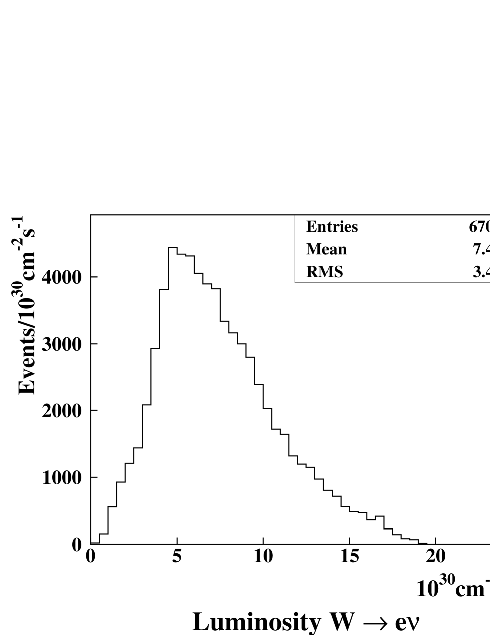
FIG. 17.: Distribution in luminosity for $W\to e\nu$ or $Z\to ee$ candidates. The mean and RMS values of the distributions are consistent with each other.

It should be noted that CDF and previous DØ measurements used different normalizations for luminosity. The CDF Collaboration bases its luminosity purely on its own measurement of the inelastic $p\overline{p}$ cross section [39, 42]. As a result, current luminosities used by CDF are 6.2% lower than those used by DØ, and consequently all DØ cross sections are ab initio 6.2% lower than all CDF cross sections. Previous DØ measurements relied only on results from CDF and E710. Including the recent E811 measurement of the inelastic $p\overline{p}$ cross section in the world average increased the discrepancy in normalization relative to CDF from 3.0% to 6.2% (i.e., current values are 3.2% higher than previous DØ measurements). The luminosity measurement used by DØ prior to the E811 result is described more extensively in Ref. [43].

VIII The Cross Sections and their Ratio

The product of the $W$ boson cross section and the branching fraction for $W\to e\nu$ is calculated using the relation

$$\sigma(p\overline{p}\rightarrow W+X)\cdot B(W\rightarrow e\nu)=\frac{N_{obs}^{W}\cdot\left(1-f_{QCD}^{W}\right)-\epsilon_{W}\cdot N_{obs}^{Z}(1-f_{QCD}^{Z})\cdot\frac{A_{Zee}^{W}+A_{Z\tau}^{W}}{A_{Z}\cdot\epsilon_{Z}}}{\epsilon_{W}\cdot A_{W}\cdot\left(1+\frac{A_{W\tau}^{W}}{A_{W}}\right)\cdot{\cal L}}$$ (15)

where $N_{obs}^{W}$ and $N_{obs}^{Z}$ are the number of $W\to e\nu$ and $Z\to ee$ candidate events, respectively; $f_{QCD}^{W}$ and $f_{QCD}^{Z}$ are the fraction of the $W\to e\nu$ and $Z\to ee$ candidate events, respectively, that come from multijet, $b$ quark, and direct photon background sources; $\epsilon_{W}$ and $\epsilon_{Z}$ are the efficiency for $W\to e\nu$ and $Z\to ee$ events, respectively, to pass the selection requirements; $A_{W}$ and $A_{Z}$ are the geometric and kinematic acceptance for $W\to e\nu$ and $Z\to ee$, respectively, which include effects from detector resolution; $A_{W\tau}^{W}$, $A_{Zee}^{W}$ and $A_{Z\tau}^{W}$ are the fraction of $W\to\tau\nu$, $Z\to ee$, and $Z\to\tau\tau$ events, respectively, that passes the $W\to e\nu$ selection criteria; and $\cal L$ is the integrated luminosity of the data sample.

The product of the $Z$ boson cross section and the branching fraction for $Z\to ee$ is determined from the relation

$$\sigma(p\overline{p}\rightarrow Z+X)\cdot B(Z\rightarrow ee)=\frac{N_{obs}^{Z}\cdot\left(1-f_{QCD}^{Z}\right)\cdot\left(1-f_{DY}\right)}{\epsilon_{Z}\cdot A_{Z}\cdot{\cal L}}$$ (16)

where $f_{DY}$ is a correction for the Drell-Yan contribution to $Z$ boson production. The ratio ${\cal R}$ can therefore be written as

$${\cal R} = \frac{\epsilon_{Z}}{\epsilon_{W}}\cdot\frac{A_{Z}}{A_{W}}\cdot\frac{1}{1+\frac{A^{W}_{W\tau}}{A_{W}}}\cdot\frac{1}{1-f_{QCD}^{Z}}\cdot\frac{1}{1-f_{DY}}$$ (17)

$$\times \left[\frac{N_{obs}^{W}}{N_{obs}^{Z}}\cdot\left(1-f_{QCD}^{W}\right)-\epsilon_{W}\cdot\frac{(A_{Zee}^{W}+A_{Z\tau}^{W})\cdot\left(1-f_{QCD}^{Z}\right)}{A_{Z}\cdot\epsilon_{Z}}\right]$$ (18)

The uncertainties on the individual cross sections are dominated by the uncertainty on the integrated luminosity measurement (4.3%). Tables V and VI summarize the results for the individual cross sections. The result for $\sigma(p\overline{p}\rightarrow W+X)\cdot B(W\rightarrow e\nu)$  is 2310 $\pm$ 10 (stat) $\pm$ 50 (syst) $\pm$ 100 (lum) pb. The result for $\sigma(p\overline{p}\rightarrow Z+X)\cdot B(Z\rightarrow ee)$ is 221 $\pm$ 3 (stat) $\pm$ 4 (syst) $\pm$ 10 (lum) pb.

TABLE V.: Values used in the $W\to e\nu$ cross section measurement.

$\sigma(p\overline{p}\rightarrow W+X)\cdot B(W\rightarrow e\nu)$	2310 $\pm$ 110 pb
	Value	Uncertainty Contribution [pb]
${N_{obs}^{W}}$	67078	10
${\epsilon_{W}}$	0.671 $\pm$ 0.009	30
${A_{W}}$	0.465 $\pm$ 0.004	20
$f_{QCD}^{W}$	0.064 $\pm$ 0.014	35
$(A_{Zee}^{W}+A_{Z\tau}^{W})/A_{Z}$	0.133 $\pm$ 0.034	–
${\epsilon_{Z}}$	0.744 $\pm$ 0.011	–
$f_{QCD}^{Z}$	0.045 $\pm$ 0.005	–
$N_{Z}^{W}$	$621\pm 155$	6
$A_{W\tau}^{W}/A_{W}$	0.0211 $\pm$ 0.0021	5
$\cal L$	84.5 $\pm$ 3.6 pb-1	100

TABLE VI.: Values used in the $Z\to ee$ cross section measurement.

$\sigma(p\overline{p}\rightarrow Z+X)\cdot B(Z\rightarrow ee)$	221 $\pm$ 11 pb
	Value	Uncertainty Contribution [pb]
${N_{obs}^{Z}}$	5397	3
${\epsilon_{Z}}$	0.744 $\pm$ 0.011	3
${A_{Z}}$	0.366 $\pm$ 0.003	2
$f_{QCD}^{Z}$	0.045 $\pm$ 0.005	1
$f_{DY}$	0.012 $\pm$ 0.001	$<1$
$\cal L$	84.5 $\pm$ 3.6 pb-1	10

Figure 18 shows a comparison between our results and calculations of order $\alpha_{s}^{2}$ using the program of Ref. [9] with the CTEQ4M structure functions, a $Z$ boson mass of 91.188 GeV, a $W$ boson mass of 80.375 GeV, and $\sin^{2}{\theta_{W}}$=0.2231. The DØ results in the muon channel [6] are from Run 1a(1992–1993), and have been multiplied by 0.969 for consistency with the new luminosity normalization.

FIG. 18.: Comparison between measured and predicted cross sections. The lines correspond to a theoretical calculation of order $\alpha_{s}^{2}$ using the program of Ref. [9] with the CTEQ4M structure functions, a $Z$ boson mass of 91.188 GeV, a $W$ boson mass of 80.375 GeV, and $\sin^{2}{\theta_{W}}$=0.2231. The DØ results in the muon channel are from Ref. [6] normalized to the new luminosity.

Figure 19 shows the Run 1b (1994–1995) results for the individual $W$ and $Z$ boson cross sections times electronic branching fraction and the previous DØ results from Run 1a (1992–1993) [6] for both the electron and muon channels compared to the corresponding theoretical predictions. The Run 1a results are normalized to the new luminosity for consistency with Run 1b results.

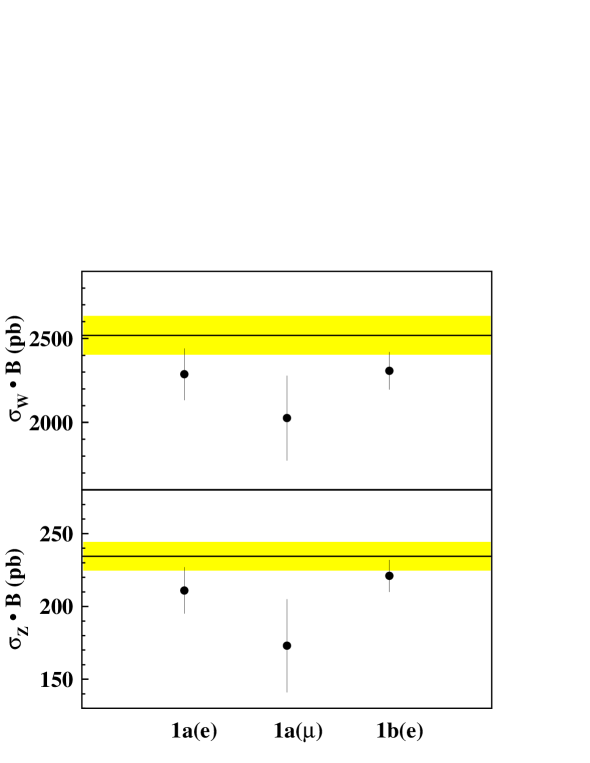
FIG. 19.: Run 1a (1992–1993) [6] and 1b (1994–1995) results for the $W$ and $Z$ boson cross sections times branching fractions. The line is the theoretical prediction from Ref. [9]. The central value uses $\Lambda_{\rm QCD}=296$ MeV and the CTEQ4M structure functions. The shaded region shows the uncertainty in the prediction due to variations in $\alpha_{s}$ obtained by varying $\Lambda_{\rm QCD}$ between 213 MeV and 399 MeV. The Run 1a results have been normalized to the new luminosity to be consistent with Run 1b results.

Table VII summarizes the result for the ratio of the cross sections, $\sigma(p\overline{p}\rightarrow W+X)\cdot B(W\rightarrow e\nu)/\sigma(p\overline{p}\rightarrow Z+X)\cdot B(Z\rightarrow ee)$.

TABLE VII.: Values used in the Ratio Measurement.

$\cal R$	10.43 $\pm$ 0.27
	Value	Uncertainty Contribution
$N_{obs}^{W}/N_{obs}^{Z}$	12.43 $\pm$ 0.18	0.15
$\epsilon_{Z}/\epsilon_{W}$	1.108 $\pm$ 0.007	0.06
$A_{Z}/A_{W}$	0.787 $\pm$ 0.007	0.09
$(A_{Zee}^{W}+A_{Z\tau}^{W})/A_{Z}$	0.133 $\pm$ 0.034	0.03
$f_{QCD}^{W}$	0.064 $\pm$ 0.014	0.16
$f_{QCD}^{Z}$	0.045 $\pm$ 0.005	0.05
$f_{DY}$	0.012 $\pm$ 0.001	0.01
$A_{W\tau}^{W}/A_{W}$	0.021 $\pm$ 0.002	0.02

In the ratio, many of the systematic uncertainties, including the luminosity uncertainty, cancel. The uncertainty in ${\cal R}$ has five main components: the uncertainty in the multijet, $b$ quark, and direct photon backgrounds to the $W$ boson (1.5%); the statistics of the $Z$ boson sample (1.4%); the uncertainty in the ratio of the $W$ and $Z$ boson acceptances (0.8%); the uncertainty in the ratio of the $W$ and $Z$ boson electron identification efficiencies (0.6%); and the uncertainty in the multijet, $b$ quark, and direct photon backgrounds to the $Z$ (0.5%). In addition, we assign a 1% uncertainty in $\cal R$ due to next-to-leading-order electroweak radiative corrections. The result is $\cal{R}=$ 10.43 $\pm$ 0.15 (stat) $\pm$ 0.20 (syst) $\pm$ 0.10 (NLO).

IX Consistency Checks

A Cross Sections from the Individual Cryostats

As a consistency check, we calculate the $W$ and $Z$ boson cross sections using the data from each calorimeter cryostat individually and compare the differences between them with the uncorrelated uncertainties. The luminosity uncertainty is 100% correlated between the different cyostats and therefore is not used in these comparisons. For the CC alone, the result for $\sigma(p\overline{p}\rightarrow W+X)\cdot B(W\rightarrow e\nu)$  is 2308 $\pm$ 11 (stat) $\pm$ 51 (syst) $\pm$ 99 (lum) pb. For the EC, the result is 2207 $\pm$ 16 $\pm$ 121 $\pm$ 95 pb. The dominant uncertainties in the CC are the uncertainty on the acceptance ($\pm$ 21 pb); the uncertainty on the efficiency ($\pm$ 31 pb); and the uncertainty from the multijet, $b$ quark, and direct photon background ($\pm$ 34 pb). The dominant uncertainties in the EC are on the acceptance ($\pm$ 20 pb); the efficiency ($\pm$ 41 pb); and the multijet, $b$ quark, and direct photon background ($\pm$ 112 pb). The uncertainties in the acceptances come from uncertainties in the calorimeter energy scales (mostly uncorrelated), assumptions on the distribution of $W$ and $Z$ boson transverse momentum (correlated), and assumptions on the effects of final state radiation (correlated). The systematic uncertainties in the efficiencies are mostly correlated. There is a statistical component that would be uncorrelated, but we neglect it here and assume the efficiencies are correlated. The uncertainties in QCD backgrounds are mostly uncorrelated between the CC and the EC. Using the full uncertainty in the background (the uncertainties in acceptance and efficiency can be neglected for the purposes of this comparison), we estimate the difference between the CC and EC cross sections as 101 $\pm$ 19 $\pm$ 117 pb.

Using only CC-CC combinations, the result for $\sigma(p\overline{p}\rightarrow Z+X)\cdot B(Z\rightarrow ee)$ is 223 $\pm$ 4 $\pm$ 4 $\pm$ 10 pb. For CC-EC combinations, it is 216 $\pm$ 5 $\pm$ 4 $\pm$ 9 pb. For EC-EC combinations, it is 235 $\pm$ 10 $\pm$ 5 $\pm$ 10 pb. The dominant uncertainty in the CC-CC  measurement is from the uncertainty on the lepton identification efficiency (3.5 pb). The dominant uncertainties in the CC-EC measurement are from lepton identification (3.3 pb) and QCD background (2.3 pb). In the EC-EC measurements, lepton identification contributes 4.5 pb to the uncertainty, and QCD background contributes 2.5 pb. To estimate the errors on the difference, we assume that the efficiencies are correlated. For the CC-CC measurement, the background contribution is small. Because the CC-EC and EC-EC backgrounds both contain an EC electron candidate, we assume the background is 100% correlated. We therefore consider only the statistical uncertainty, and we get $\sigma_{{\rm CC-CC}}-\sigma_{{\rm CC-EC}}=7\pm 6$ pb, $\sigma_{{\rm CC-CC}}-\sigma_{{\rm EC-EC}}=-12\pm 11$ pb, and $\sigma_{{\rm CC-EC}}-\sigma_{{\rm EC-EC}}=-19\pm 11$ pb.

B Dependence on Instantaneous Luminosity

To search for any dependences on luminosity, the data are divided into five subsamples according to the value of the instantaneous luminosity when each event occurred so that each subsample contains approximately one fifth of the events. The mean values of the instantaneous luminosity for each sample are 3.33, 5.40, 7.24, 9.43, and 13.29 $\times 10^{30}$ cm^-2s^-1. For each subsample, the electron identification efficiencies; the integrated luminosity; and the backgrounds from multijet, $b$ quarks, and direct photons were re-calculated. The electron identification efficiency for $W$ boson events for the highest luminosity bin is 17% lower than that for the lowest luminosity bin, and the multijet background is 2% larger. Figures 20 and 21 show the $W$ and $Z$ boson cross section, respectively, as a function of luminosity. Figure 22 shows the ratio of cross sections in the five bins of instantaneous luminosity. The observed cross sections and their ratio do not appear to depend on instantaneous luminosity, as the data are statistically consistent with no luminosity dependence.

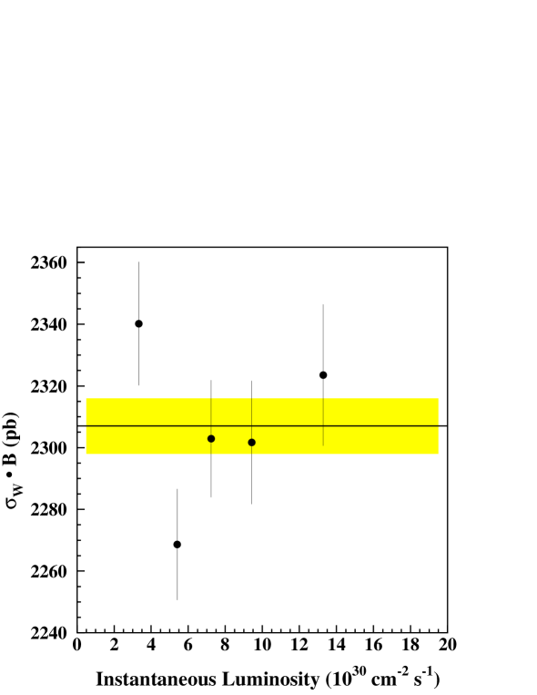
FIG. 20.: The $W\to e\nu$ cross section versus instantaneous luminosity. The error bars are statistical only. The solid line is the result from summing over all instantaneous luminosities and the shaded band is the corresponding statistical uncertainty.

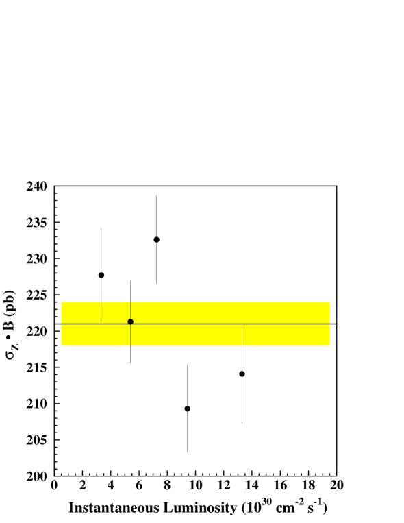
FIG. 21.: The $Z\to ee$ cross section versus instantaneous luminosity. The error bars are statistical only. The solid line is the result from summing over all instantaneous luminosities and the shaded band is the corresponding statistical uncertainty.

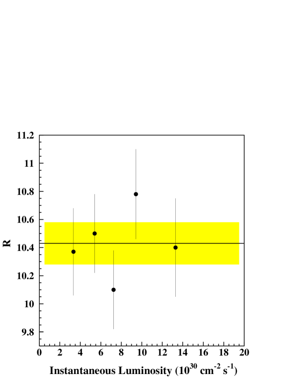
FIG. 22.: The ratio $\sigma(p\overline{p}\rightarrow W+X)\cdot B(W\rightarrow e\nu)/\sigma(p\overline{p}\rightarrow Z+X)\cdot B(Z\rightarrow ee)$ versus instantaneous luminosity. The error bars are statistical only. The solid line is the result from summing over all instantaneous luminosities and the shaded band is the corresponding statistical uncertainty.

X $\sigma(p\overline{p}\rightarrow W+X)\cdot B(W\rightarrow e\nu)$ at $\sqrt{s}=630$ GeV

We measure the $W\to e\nu$ cross section using data from a short Tevatron run at a center-of-mass energy $\sqrt{s}=630$ GeV [44]. The integrated luminosity is calculated in the same way as for the $\sqrt{s}=1800$ GeV sample, except that we use values of $\sigma_{sd}$, $\sigma_{dd}$, and $\sigma_{nd}$ which correspond to a center-of-mass energy of 630 GeV. These values are obtained by interpolating between the measured values at $\sqrt{s}=1800$ GeV and at $\sqrt{s}=546$ GeV, and their uncertainties are dominated by the uncertainties at 546 GeV. The luminosity calculation at $\sqrt{s}=630$ GeV is described in Ref. [45]. The integrated luminosity is 505 $\pm$ 15 nb^-1. The cross section for inclusive $W$ boson production at this center-of-mass energy has previously been measured by the UA1 [46] and UA2 [47] collaborations. We use the same $W\to e\nu$ selection criteria as was used for the measurement at $\sqrt{s}=1800$ GeV, and find a total of 130 $W\to e\nu$ candidate events, 119 of which have their electron in the CC calorimeter.

Since the 630 GeV data sample contains very few $Z\to ee$ candidates (approximately 10), we do not use this sample to obtain the electron identification efficiency. Instead, we extrapolate the efficiency from the 1800 GeV sample. The efficiency depends on the number of jets in the $W\to e\nu$ event and on the ambient energy in the event. The 130 events from the $W\to e\nu$ sample taken at $\sqrt{s}=630$ GeV contain no jets with $E_{T}>25$ GeV. Figure 23 shows, for the $W\to e\nu$ sample taken at $\sqrt{s}=1800$ GeV, the electron identification efficiency for events without jets with $E_{T}>25$ GeV as a function of the mean energy per unit of rapidity and per unit of azimuthal angle $\phi$. The data sample taken at $\sqrt{s}=630$ GeV has a mean energy density of 1.3 GeV$/\eta/\phi$, where $\phi$ is in radians. We fit the curve from the 1800 GeV data to a first-order polynomial and use the fit to extrapolate to this energy density to obtain the efficiency of the electron identification requirements. We obtain an electron identification efficiency of 0.808 $\pm$ 0.024, where the uncertainty comes from the uncertainty in the fit. The efficiency of the LØ trigger for $W$ boson events relative to that for minimum bias events is also scaled from the result at 1800 GeV. The LØ trigger efficiency for minimum bias events at 1800 GeV is 0.905 and at 630 GeV is 0.823. The $W$ boson efficiency is scaled by the ratio of these two numbers and is 0.897 $\pm$ 0.009.

FIG. 23.: The efficiency for the electron identification criteria in the CC and EC. Each is measured as a function of the energy density in the event for events containing no jets with $E_{T}$$>$ 25 GeV as evaluated using the $Z\to ee$ sample taken at $\sqrt{s}$=1800 GeV. The mean energy density of the sample taken at $\sqrt{s}=630$ GeV is 1.3 GeV$/\eta/\phi$.

The kinematic and fiducial acceptance is evaluated using the same simulation as was used for the measurement at 1800 GeV. The fraction of $W\to e\nu$ events passing our fiducial and kinematic requirements at 630 GeV is 0.521 $\pm$ 0.013.

The background from multijets, $b$ quarks, and direct photons is calculated by scaling the 1800 GeV result, using $\displaystyle{f_{QCD}^{630}={P^{630}\over P^{1800}}\cdot{\sigma_{j}^{630}\over\sigma_{w}^{630}}\cdot{\sigma_{w}^{1800}\over\sigma_{j}^{1800}}}$, where $P$ is the probability for a jet to fake an electron, $\sigma_{j}$ is the cross section for jets with smeared $p_{T}>25$ GeV, and $\sigma_{w}$ is the $W$ boson cross section. The JETRAD [48] program together with a parameterization of the response of the detector has been shown to be in good agreement with the data [49]. Using this program, we find $\displaystyle{{\sigma_{j}^{630}\over\sigma_{w}^{630}}\cdot{\sigma_{w}^{1800}\over\sigma_{j}^{1800}}=0.28\ \pm 0.11}$ and $\displaystyle{{P^{630}\over P^{1800}}=1.5}$, giving $f_{QCD}^{630}$= 0.016 $\pm$ 0.012. The uncertainty is dominated by the uncertainty in the jet cross section from JETRAD. The fraction of the candidates from the other sources of background ($W\to\tau\nu$, $Z\to ee$, $Z\to\tau\tau$) is assumed to scale in the same way as the signal with center-of-mass energy. Since 621 $Z$ boson events are expected to fake $W$ boson events at 1800 GeV, we expect 621 $\cdot$ 130 $/$ 67078 $=$ 1.2 $\pm$ 0.3 $Z$ boson events to pass the $W$ boson selection at 630 GeV.

Table VIII and Figs. 24 and 18 summarize our result. The result for $\sigma(p\overline{p}\rightarrow W+X)\cdot B(W\rightarrow e\nu)$  is 658 $\pm$ 58 (stat) $\pm$ 34 (syst) pb, where the systematic uncertainty includes a 3.0% uncertainty in the integrated luminosity.

TABLE VIII.: Values used in the $W\to e\nu$ cross section measurement at 630 GeV.

	$\sigma(p\overline{p}\rightarrow W+X)\cdot B(W\rightarrow e\nu)$	658 $\pm$ 67 pb
	${N_{obs}^{W}}$	130
	${\epsilon_{W}}$	0.799 $\pm$ 0.024
	LØ	0.897 $\pm$ 0.009
	${A_{W}}$	0.521 $\pm$ 0.013
	$Z$ boson background	1.2 $\pm$ 0.3
	$(A_{Zee}^{W}+A_{Z\tau}^{W})/A_{Z}$	0.133 $\pm$ 0.034
	$f_{QCD}^{W}$	0.016 $\pm$ 0.012
	$A_{W\tau}^{W}/A_{W}$	0.021 $\pm$ 0.002
	$\cal L$	505 $\pm$ 15 nb-1

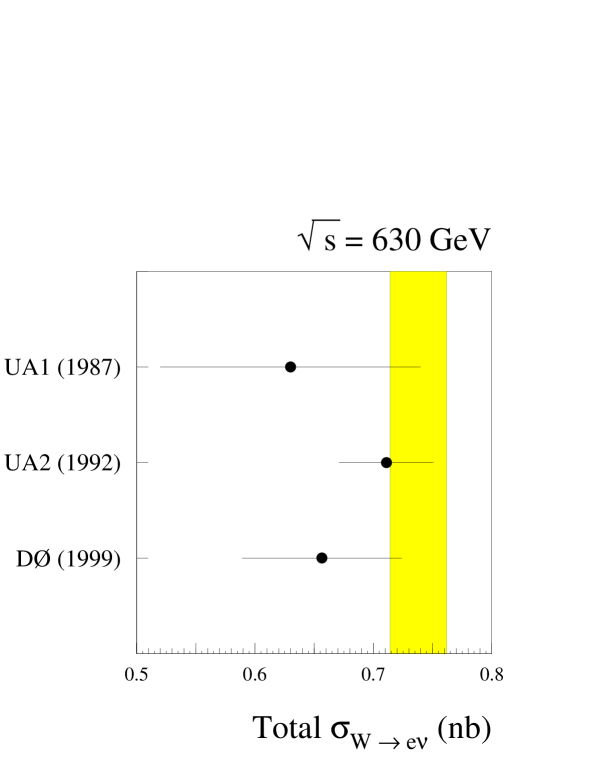
FIG. 24.: Measurements of the $W$ boson inclusive cross section times electronic branching fraction at a center-of-mass energy of 630 GeV. Our result is in good agreement with previous measurements from the UA1 [46] and UA2 [47] collaborations. The shaded band is a NLO prediction from the code of Ref. [9] with the CTEQ2M parton distribution functions, a $Z$ boson mass of 91.190 GeV, a $W$ boson mass of 80.23 GeV, and $\sin{\theta_{W}}^{2}=$ 0.2259.

XI The Electronic Branching Fraction, Width, and Invisible Width of the $W$ Boson

Using the results $\sigma(p\overline{p}\rightarrow W+X)\cdot B(W\rightarrow e\nu)$ = 2310 $\pm$ 10 $\pm$ 50 $\pm$ 100 pb, $\sigma(p\overline{p}\rightarrow Z+X)\cdot B(Z\rightarrow ee)$ = 221 $\pm$ 3 $\pm$ 4 $\pm$ 10 pb, and ${\cal R}=10.43\ \pm 0.15\ \pm 0.20\pm 0.10$, we can determine the electronic branching fraction of the $W$ boson via

$$B(W\rightarrow e\nu)={\cal R}\cdot B(Z\rightarrow ee)\cdot\frac{\sigma_{Z}}{\sigma_{W}}$$ (19)

Using $B(Z\rightarrow ee)$ = 0.03367 $\pm$ 0.00006 [50] and $\sigma_{W}/\sigma_{Z}$ = 3.29 $\pm$ 0.03 [9], we get $B(W\rightarrow e\nu)$ = 0.1066 $\pm$ 0.0015 (stat) $\pm$ 0.0021 (syst) $\pm$ 0.0011 (other) $\pm$ 0.0011 (NLO), where the next-to-last source of uncertainty comes from uncertainties in $B(Z\rightarrow ee)$ and in $\sigma_{W}/\sigma_{Z}$. The standard model prediction is $B(W\rightarrow e\nu)=0.1084\pm 0.0002$. Assuming the standard model prediction for the electronic partial width (0.2270 $\pm$ 0.0011 GeV [51]), we can calculate the $W$ boson width $\Gamma_{W}=\Gamma_{W}^{e}/B(W\rightarrow e\nu)$ as 2.130 $\pm$ 0.030 (stat) $\pm$ 0.041 (syst) $\pm$ 0.022 (other) $\pm$ 0.021 (NLO) GeV, to be compared with the standard model prediction of $\Gamma_{W}$ = 2.094 $\pm$ 0.006 GeV [51]. The difference between our measured value and the standard model prediction, which is the width for the $W$ boson to decay to final states other than the two lightest quark doublets and the three lepton doublets, is thus 0.036 $\pm$ 0.060 GeV. This is consistent with zero within uncertainties, so we set a 95% confidence level upper limit on the $W$ boson width to non-standard-model final states (“invisible width”). Assuming the uncertainty is Gaussian, removing the unphysical region where the invisible width is negative, and integrating to 95% of the remaining area, we set a 95% confidence level upper limit on the invisible partial width of the $W$ boson of 0.168 GeV.

We combine our Run 1b (1994–1995) result with the DØ results from Run 1a (1992–1993) [6] for $\cal R$. Table IX compares the two measurements.

TABLE IX.: Comparison of the current Run 1b (1994–1995) measurement to the Run 1a (1992–1993) measurement.

Data Period	$\cal R$	Correlated uncertainty	Uncorrelated uncertainty
1a,electron (13 pb-1)	10.82	0.141	0.408
1a,muon (11 pb-1)	11.8	0	2.110
1b,electron (84.5 pb-1)	10.43	0.141	0.235

Because most of the systematic uncertainties in the Run 1a measurement in the electron channel were dominated by the statistics of the sample used to evaluate the uncertainty, the 1a and 1b measurements in the electron channel are mostly uncorrelated. Only the acceptance, the Drell-Yan correction, and the NLO uncertainties are correlated (we have added the same 1% NLO uncertainty to the 1a result). The measurements in the muon and electron channels are uncorrelated. With this assumption, we get ${\cal R}=10.54\pm 0.24$, $\Gamma_{W}=2.107\pm 0.054\$ GeV, and a 95% confidence level upper limit on the invisible width of 0.132 GeV. Table X summarizes our results.

TABLE X.: Results.

	1b	1a+1b combined
	(84.5 pb-1)	(13 + 11 + 84.5 pb-1)
Ratio $\cal R$	10.43 $\pm$ 0.27	10.54 $\pm$ 0.24
$B(W\rightarrow e\nu)$	0.1066 $\pm$ 0.0030	0.108 $\pm$ 0.003
$\Gamma_{W}$	2.130 $\pm$ 0.060 GeV	2.107 $\pm$ 0.054 GeV
95% C.L. upper limit $\Gamma_{W}^{inv}$	0.168 GeV	0.132 GeV

XII Conclusions

We have presented new measurements of $\sigma(p\overline{p}\rightarrow W+X)\cdot B(W\rightarrow e\nu)$ and $\sigma(p\overline{p}\rightarrow Z+X)\cdot B(Z\rightarrow ee)$ using 84.5 pb^-1 of data. We determine $\sigma(p\overline{p}\rightarrow W+X)\cdot B(W\rightarrow e\nu)$ $=2310\pm 110$ pb and $\sigma(p\overline{p}\rightarrow Z+X)\cdot B(Z\rightarrow ee)$ $=221\pm 11$ pb. The uncertainty in these measurements is dominated by the luminosity uncertainty. From these measurements, we have derived the ratio ${\cal R}=10.43\pm 0.27$ and a new indirect measurement of the total $W$ boson width, $\Gamma_{W}=2.130\pm 0.060$ GeV. We obtain a 95% confidence level upper limit on the invisible $W$ boson width of 168 MeV. Combining these results with those from the 1992–1993 run [6], we determine ${\cal R}=10.54\pm 0.24$, $\Gamma_{W}=2.107\pm 0.054\$ GeV, and a 95% confidence level upper limit on the invisible width of 0.132 GeV.

REFERENCES

- [1] G. Arnison et al. (UA1 Collaboration), Phys. Lett. B 122, 103 (1983); M. Banner et al. (UA2 Collaboration), Phys. Lett. B 122, 476 (1983); P. Bagnaia et al. (UA2 Collaboration), Phys. Lett. B 129, 130 (1983); G. Arnison et al. (UA1 Collaboration), Phys. Lett. B 129, 273 (1983).
- [2] S. Abachi et al. (DØ Collaboration), Phys. Rev. Lett. 75, 1023 (1995); S. Abachi et al. (DØ Collaboration), Phys. Rev. Lett. 77, 3303 (1996); S. Abachi et al. (DØ Collaboration), Phys. Rev. Lett. 77, 3309 (1996); S. Abachi et al. (DØ Collaboration), Phys. Rev. Lett. 78, 3634 (1997); B. Abbott et al. (DØ Collaboration), Phys. Rev. Lett. 79, 1441 (1997); B. Abbott et al. (DØ Collaboration), Phys. Rev. Lett. 80, 5498 (1998); F. Abe et al. (CDF Collaboration), Phys. Rev. Lett. 75 11 (1995); F. Abe et al. (CDF Collaboration), Phys. Rev. Lett. 75 1017 (1995); F. Abe et al. (CDF Collaboration), Phys. Rev. Lett. 74 850 (1995); F. Abe et al. (CDF Collaboration), Phys. Rev. Lett. 74 341 (1995); F. Abe et al. (CDF Collaboration), Phys. Rev. Lett. 74 1936 (1995); P. Abreu et al. (DELPHI Collaboration), Phys. Lett. B 416, 233 (1998); R. Barate et al. (ALEPH Collaboration), Phys. Lett. B 415, 435 (1997); M. Acciarri et al. (L3 Collaboration), Phys. Lett. B 407 419 (1997); R. Barate et al. (ALEPH Collaboration), Phys. Lett. B 401, 347 (1997); M. Acciarri et al. (L3 Collaboration), Phys. Lett. B 398, 223 (1997); P. Abreu et al. (DELPHI Collaboration), Phys. Lett. B 397, 158 (1997).
- [3] C. Albajar et al. (UA1 Collaboration), Phys. Lett. B 253, 503 (1991).
- [4] J. Alitti et al. (UA2 Collaboration), Phys. Lett. B 276, 365 (1992).
- [5] F. Abe et al. (CDF Collaboration), Phys. Rev. D 52, 2624 (1995).
- [6] S. Abachi et al. (DØ Collaboration), Phys. Rev. Lett. 75, 1456 (1995); B. Abbott et al. (DØ Collaboration), submitted to Phys. Rev. D, hep-ex/9901040.
- [7] M. Acciarri et al. (L3 Collaboration), “Measurement of Mass and Width of the Boson at LEP”, CERN-EP/99-17, accepted by Phys. Lett. B; G. Abbiendi et al. (OPAL Collaboration), “Measurement of the Mass and Width in Collisons at 183 GeV”, CERN-EP/98-197 (1998);
- [8] J. Kalinowski and P. M. Zerwas, Phys. Lett. B 400, 112 (1997).
- [9] R. Hamberg, W.L. van Neerven and T. Matsuura, Nucl. Phys. B359, 343 (1991); W.L. van Neerven and E.B. Zijlstra, Nucl. Phys. B382, 11 (1992).
- [10] P. Abreu et al. (DELPHI Collaboration), Nucl. Phys. B418, 403 (1994); M. Acciarri et al. (L3 Collaboration), Z. Phys. C62, 551 (1994); R. Akers et al. (OPAL Collaboration), Z. Phys. C61, 19 (1994); D. Buskulic et al. (ALEPH Collaboration), Z. Phys. C62, 539 (1994).
- [11] F. Abe et al. (CDF Collaboration), Phys. Rev. Lett. 74, 341 (1995).
-
[12]
J. Tarazi, Ph.D. thesis, University of
California at Irvine, 1997 (unpublished),
http://www-d0.fnal.gov/results/publications_talks/thesis/tarazi/thesis_final_2side.ps. - [13] G. Gómez, Ph.D. thesis, University of Maryland, 1999 (in preparation).
- [14] S. Abachi et al. (DØ Collaboration), Nucl. Instrum. Methods in Phys. Res. A 338, 185 (1994).
- [15] M. Abolins et al. (DØ Collaboration), Nucl. Instrum. Methods in Phys. Res. A 280, 36 (1989); S. Abachi et al. (DØ Collaboration), ibid. 324, 53 (1993); H. Aihara et al. (DØ Collaboration), ibid. 325, 393 (1993).
- [16] The LEP Collaborations, the LEP Electroweak Working Group, and the SLD Heavy Flavour Group, CERN-PPE/96-183 (unpublished).
- [17] B. Abbott et al. (DØ Collaboration), Phys. Rev. D 58, 092003 (1998).
-
[18]
E.M. Flattum, Ph.D. thesis, Michigan State University, 1996 (unpublished),
http://www-d0.fnal.gov/results/publications_talks/thesis/flattum/eric_thesis.ps. -
[19]
I.M. Adam, Ph.D. thesis, Columbia University, 1997 (unpublished),
http://www-d0.fnal.gov/results/publications_talks/thesis/adam/ian_thesis_all.ps. - [20] J. Botts et al. (CTEQ Collaboration), Phys. Lett. B 304, 159 (1993); H.L. Lai et al. (CTEQ Collaboration), Phys. Rev. D 51, 4763 (1995); H.L. Lai et al. (CTEQ Collaboration), Phys. Rev. D 55, 1280 (1997).
- [21] G.A. Ladinsky and C.-P. Yuan, Phys. Rev. D 50, 4239 (1994).
- [22] F.A. Berends and R. Kleiss, Z. Phys. C27, 365 (1985).
- [23] T. Sjöstrand, Comput. Phys. Commun. 82, 74 (1994).
- [24] F. Abe et al. (CDF Collaboration), Phys. Rev. Lett. 75, 11 (1995) and Phys. Rev. D 52, 4784 (1995).
- [25] A.D. Martin, W.J. Stirling, and R.G. Roberts, Phys. Lett B 306, 145 (1993).
- [26] A.D. Martin, W.J. Stirling, and R.G. Roberts, Phys. Lett. B 354, 155 (1995).
- [27] M. Gluck, E. Reya, and A. Vogt, Z. Phys. C53, 127 (1992).
- [28] A.D. Martin, W.J. Stirling, and R.G. Roberts, Phys. Lett. 356B, 89 (1995).
- [29] F. Paige and S.D. Protopopescue, in Supercollider Physics, edited by D. Soper (World Scientific, Singapore, 1987), p.41; and Brookhaven National Laboratory Report No. 38304, 1986 (unpublished).
- [30] U. Baur, S. Keller, and D. Wackeroth, FERMILAB-PUB-98164-T, hep-ph/9807417; U. Baur, S. Keller, and W.K. Sakumoto, Phys. Rev. D 57, 199 (1998).
- [31] U. Baur, private communication.
- [32] R. Brun and F. Carminati, CERN Program Library Long Writeup W5013, 1993 (unpublished).
- [33] An example may help make this cancelation more intuitive. Suppose that most of the time, the probability that one of the electrons in a boson event passes the tracking cuts is uncorrelated with the probability that the other electron passes. If, for certain runs, a detector malfunction were to cause all tracking to fail, the probability that one electron fails (100%) is 100% correlated with the probability that the other fails (100%). Since all and boson events that occur during this hardware failure would be lost, the loss cancels in the ratio.
- [34] F. Abe et al. (CDF Collaboration), Phys. Rev. Lett. 78, 2698 (1997).
- [35] L. Alvero, J.C. Collins, J. Terron, and J.J. Whitmore, Phys. Rev. D 59, 74022 (1999).
- [36] S. Abachi et al. (DØ Collaboration), Phys. Rev. D 52, 4877 (1995).
- [37] G. Marchesini et al., Comput. Phys. Commun. 67, 465 (1992), and hep-ph/9607393, release 5.7. (unpublished).
- [38] Luminosity measurements are stored periodically (every minute) and then integrated over the live running time. This one-minute period is much shorter than the time it takes for the luminosity to change significantly.
- [39] F. Abe et al. (CDF Collaboration), Phys. Rev. D 50, 5550 (1994).
- [40] N. Amos et al. (E710 Collaboration), Phys. Rev. Lett. 68, 2433 (1992).
- [41] C. Avila et al. (E811 Collaboration), Phys. Lett. B 445, 419 (1999).
- [42] M. Albrow, A. Beretvas, P. Giromini, L. Nodulman, FERMILAB-TM-2071, 1999 (unpublished).
- [43] J. Bantly, A. Brandt, R. Partridge, J. Perkins, and D. Puseljic, FERMILAB-TM-1930, 1995 (unpublished).
-
[44]
J. Krane, Ph.D. thesis, University of Nebraska, 1998 (unpublished),
http://fnalpubs.fnal.gov/techpubs/theses.html - [45] J. Bantly, J. Krane, and D. Owen, FERMILAB-TM-2000, 1997 (unpublished).
- [46] C. Albajar et al. (UA1 Collaboration), Phys. Lett. B 198, 271 (1987).
- [47] J. Alitti et al. (UA2 Collaboration), Phys. Lett. B 276, 365 (1992).
- [48] W.T. Giele, E.W.N. Glover and D.A. Kosower, Nucl. Phys. B403, 2121 (1990).
- [49] B. Abbott et al. (DØ Collaboration), Phys. Rev. Lett. 80, 666 (1998).
- [50] L. Montanet et al. (Particle Data Group), Phys. Rev. D 54, 1 (1996).
- [51] J.L. Rosner, M.P. Worah, and T. Takeushi, Phys. Rev. D 49, 1363 (1994).